Asteroid families in the first order resonances with Jupiter

Abstract

Asteroids residing in the first-order mean motion resonances with Jupiter hold important information about the processes that set the final architecture of giant planets. Here we revise current populations of objects in the J2/1 (Hecuba-gap group), J3/2 (Hilda group) and J4/3 (Thule group) resonances. The number of multi-opposition asteroids found is $274$ for J2/1, $1197$ for J3/2 and $3$ for J4/3. By discovering a second and third object in the J4/3 resonance, (186024) 2001 QG₂₀₇ and (185290) 2006 UB₂₁₉, this population becomes a real group rather than a single object. Using both hierarchical clustering technique and colour identification we characterise a collisionally-born asteroid family around the largest object (1911) Schubart in the J3/2 resonance. There is also a looser cluster around the largest asteroid (153) Hilda. Using $N$-body numerical simulations we prove that the Yarkovsky effect (infrared thermal emission from the surface of asteroids) causes a systematic drift in eccentricity for resonant asteroids, while their semimajor axis is almost fixed due to the strong coupling with Jupiter. This is a different mechanism from main belt families, where the Yarkovsky drift affects basically the semimajor axis. We use the eccentricity evolution to determine the following ages: $(1.7\pm 0.7)\,{\rm Gyr}$ for the Schubart family and $\gtrsim 4\,{\rm Gyr}$ for the Hilda family. We also find that collisionally-born clusters in the J2/1 resonance would efficiently dynamically disperse. The steep size distribution of the stable population inside this resonance could thus make sense if most of these bodies are fragments from an event older than $\simeq 1$ Gyr. Finally, we test stability of resonant populations during Jupiter’s and Saturn’s crossing of their mutual mean motion resonances. In particular we find primordial objects in the J3/2 resonance were efficiently removed from their orbits when Jupiter and Saturn crossed their 1:2 mean motion resonance.

1 Introduction

Populations of asteroids in the Jovian first order mean motion resonances –J2/1, J3/2 and J4/3– are closely linked to the orbital evolution of the giant planets. This is because of their orbital proximity to Jupiter. Stability or instability of these asteroid populations directly derives from the orbital configuration of the giant planets. As such it is also sensitive on the nature and amount of Jupiter’s migration and other finer details of its dynamics. As a result, the currently observed asteroids in the Jovian first order resonances contain valuable information about the early evolution of planets and, if correctly understood and properly modelled, they may help to constrain it.

Apart from the Trojan clouds (not studied in this paper) the largest known population in the Jovian mean motion resonances occupies the J3/2 resonance, and is frequently called the Hilda group. It was carefully studied in a parallel series of papers by Schubart and Dahlgren and collaborators during the past few decades. Schubart (1982a,b, 1991) analysed short-term dynamics of Hilda-type orbits and introduced quasi-constant orbital parameters that allowed their first classification. While pioneering, Schubart’s work had the disadvantage of having much smaller sample of known asteroids and computer power than today. Dahlgren & Lagerkvist (1995) and Dahlgren et al. (1997, 1998, 1999) conducted the first systematic spectroscopic and rotation-rate investigation of Hildas. They found about equal abundance of D- and P-type asteroids and suggested spectral-size correlation such that P-types dominate large Hildas and D-type dominate smaller Hildas. They also suggested small Hildas have large lightcurve amplitudes, as an indication of elongated or irregular shape, and that the distribution of their rotation rates is non-Maxwellian. Further analysis using the Sloan Digital Sky Survey (SDSS) data however does not support significant dominance of either of the two spectral types for small sizes and indicates about equal mix of them (Gil-Hutton & Brunini 2008; see also below). Smaller populations of asteroids in the J2/1 and J4/3 received comparatively less observational effort.

Since the late 1990s powerful-enough computers allowed a more systematic analysis of fine details of the longer-term dynamics in the Jovian first order resonances. Ferraz-Mello & Michtchenko (1996) and Ferraz-Mello et al. (1998a,b) determined that asteroids in the J2/1 resonance can be very long-lived, possibly primordial, yet their motion is comparatively more chaotic than those in the J3/2 resonance. The latter paper showed that commensurability between the libration period and the period of Jupiter’s and Saturn’s Great Inequality might have played an important role in depletion of the J2/1 resonance. This would have occurred when both giant planets were farther from their mutual 2:5 mean motion configuration in the past. A still more complete analysis was obtained by Nesvorný & Ferraz-Mello (1997) who also pointed out that the J4/3 resonance stable zone is surprisingly void of asteroids, containing only (279) Thule. Roig et al. (2001) and Brož et al. (2005) recently revised the population of asteroids in the J2/1 resonance and classified them into several groups according to their long-term orbital stability. While the origin of the unstable resonant population was successfully interpreted using a model of a steady-state flow of main belt objects driven by the Yarkovsky semimajor axis drift, the origin of the long-lived asteroids in the J2/1 remains elusive. Population of Hildas and Thule was assumed primordial or captured by an adiabatic migration of Jupiter (e.g., Franklin et al. 2004).

It has been known for some time that the current configuration of giant planets does not correspond to that at their birth. However, a new momentum to that hypothesis was given by the so called Nice model (Tsiganis et al. 2005; Morbidelli et al. 2005; Gomes et al. 2005). The Nice model postulates the initial configuration of the giant planets was such that Jupiter and Saturn were interior of their mutual 1:2 mean motion resonance (see also Morbidelli et al. 2007). The event of crossing this resonance had a major influence on the final architecture of giant planets and strongly influenced structure of small-bodies populations in the Solar system. Morbidelli et al. (2005) showed that the population of Jupiters Trojan asteroids was destabilised and re-populated during this phase. In what follows we show that, within the Nice model, the same most probably occurs for populations of asteroids in the J3/2 and J4/3 resonances.

The paper is organised as follows: in Section 2 we revise information about the current populations of asteroids in the Jovian first order resonances. We use an up-to-date AstOrb database of asteroid orbits from the Lowell Observatory (ftp.lowell.edu) as of September 2007 and eliminate only single-opposition cases to assure accurate orbital information.

In Section 3 we apply clustering techniques and extract two families of asteroids on similar orbits in the J3/2 resonance. We strengthen their case with an additional colour analysis using the SDSS broadband data. We model the long-term orbital evolution of these families and estimate their ages on the basis of Yarkovsky-driven dispersion in eccentricity.

In Section 4 we determine an orbital stability of the putative primordial populations of planetesimals in the Jovian first-order resonances. We show that those in the J3/2 and J4/3 are very efficiently eliminated when Jupiter and Saturn cross their mutual 1:2 mean motion resonance. We also determine the removal rate of very small resonant asteroids due to the Yarkovsky/YORP effects.

2 Current asteroid populations in the Jovian first order resonances

Dynamics of asteroid motion in the Jovian first order resonances has been extensively studied by both analytical and numerical methods in the past few decades (e.g., Murray 1986; Sessin & Bressane 1988; Ferraz-Mello 1988; Lemaitre & Henrard 1990; Morbidelli & Moons 1993; Moons et al. 1998; Nesvorný & Ferraz-Mello 1997; Roig et al. 2002; Schubart 2007). In what follows we review a minimum information needed to understand our paper, referring an interested reader to the literature mentioned above for more insights.

In the simplest framework of a circular restricted planar three-body problem (Sun-Jupiter-asteroid) the fundamental effects of the resonant dynamics is reduced to a one-degree of freedom problem defined by a pair of variables $(\Sigma,\sigma)$. For J$(p+1)/p$ resonance ($p=1,2$ and $3$ in our cases) we have

$$\Sigma = \sqrt{a}\,\left(1-\sqrt{1-e^{2}}\right)\;,$$ (1)

$$\sigma = \left(p+1\right)\lambda^{\prime}-p\,\lambda-\varpi\;,$$ (2)

where $a$ is the semimajor axis, $e$ the eccentricity, $\varpi$ the longitude of pericentre and $\lambda$ the mean longitude in orbit of the asteroid, and $\lambda^{\prime}$ is the mean longitude in orbit of Jupiter.

If the asteroid motion is not confined into the orbital plane of the planet, we have an additional pair of resonant variables $(\Sigma_{z},\sigma_{z})$ such that

$$\Sigma_{z} = 2\sqrt{a\left(1-e^{2}\right)}\sin^{2}\frac{i}{2}\;,$$ (3)

$$\sigma_{z} = \left(p+1\right)\lambda^{\prime}-p\,\lambda-\Omega\;,$$ (4)

where $i$ denotes the inclination of asteroids orbit and $\Omega$ the longitude of its node. Remaining still with the simple averaged model, orbital effects with shorter periods are neglected, the motion obeys an integral of motion $N$ given by

$$N=\sqrt{a}\,\left(\frac{p+1}{p}-\sqrt{1-e^{2}}\cos i\right)\;.$$ (5)

Because of this integral of motion, variations of $\Sigma$ imply oscillations of both $a$ and $e$.

The two-degree of freedom character of the resonant motion prevents integrability. However, as an approximation we may introduce a hierarchy by noting that perturbation described by the $(\Sigma,\sigma)$ variables is larger than that described by the $(\Sigma_{z},\sigma_{z})$ terms (e.g., Moons et al. 1998). This is usually true for real resonant asteroids of interest. Only the angle $\sigma$ librates and $\sigma_{z}$ circulates with a very long period. The $(\Sigma_{z},\sigma_{z})$ dynamics thus produces a long-period perturbation of the $(\Sigma,\sigma)$ motion.

Within this model the minimum value of $\Sigma$ in one resonant cycle (typically several hundreds of years) implies $a$ is minimum and $e$ is maximum. These values do not conserve exactly from one cycle to another because the $(\Sigma_{z},\sigma_{z})$ motion produces small oscillations. Since $\Sigma+\Sigma_{z}-N=-\sqrt{a}/p$ one needs to wait until $\Sigma_{z}$ reaches maximum over its cycle to attain ‘real’ minimum of $a$ values and ‘real’ maximum of $e$ values over a longer time interval. From (3) we note the maximum of $\Sigma_{z}$ occurs for the maximum of $i$ variations. This situations occurs typically once in a few thousands of years. In an ideal situation, these extremal values of $(a,e,i)$ would be constant and may serve as a set of proper orbital elements.

The motion of real asteroids in the Solar system is further complicated by Jupiter having non-zero and oscillating value of eccentricity. This brings further perturbations (e.g., Ferraz-Mello 1988; Sessin & Bressane 1988 for a simple analytic description) and sources of instability inside the resonance. Despite the non-integrability, we follow Roig et al. (2001) and introduce pseudo-proper orbital elements $(a_{p},e_{p},\sin i_{p})$ as the osculating elements $(a,e,\sin i)$ at the moment, when the orbit satisfies the condition:

$$\sigma=0\land{d\sigma\over dt}<0\land\varpi-\varpi^{\prime}=0\land\Omega-\Omega^{\prime}=0\;,$$ (6)

where $\varpi^{\prime}$ and $\Omega^{\prime}$ denote the longitude of pericentre and the longitude of node of Jupiter. As above, when (6) holds the osculating orbital elements are such that $a$ attains minimum, $e$ attains maximum and $i$ attains maximum. Numerical experiments show that with a complete perturbation model and a finite time-step it is difficult to satisfy all conditions of (6) simultaneously. Following Roig et al. (2001) we thus relax (6) to a more practical condition

$$|\sigma|<5^{\circ}\land{\Delta\sigma\over\Delta t}<0\land|\varpi-\varpi^{\prime}|<5^{\circ}\;.$$ (7)

Because this condition is only approximate, we numerically integrate orbits of resonant asteroids for 1 Myr, over which the pseudo-proper orbital elements are recorded. We then compute their mean value and standard deviation, which is an expression of the orbital stability over that interval of time.

In the case of the J3/2 and J4/3 resonances, we use the condition (7) with a different sign ${\Delta\sigma\over\Delta t}>0$ and, moreover, we apply a digital filter (denoted as A in Quinn et al. (1991), using 1 yr sampling and a decimation factor of 10) to $\sigma(t)$. This intermediate stage serves to suppress oscillations faster than the libration period. The different sign of ${\Delta\sigma\over\Delta t}$ just means our pseudo-proper orbital elements correspond to maximum value of $a$ and minimum values of $e$ and $i$, in order to allow more direct comparison with previous analyses.

Aside to this short-term integration we perform long-term runs to determine the stability of a particular resonant orbit. With this aim we conduct integrations spanning 4 Gyr for all resonant asteroids. Because of the inherent uncertainty in the initial conditions (orbital elements at the current epoch), we perform such integration for the nominal orbit and $10$ clones that randomly span the uncertainty ellipsoid. We then define dynamical lifetime of the orbit as the median of time intervals, for which the individual clones stayed in the resonance.

All integrations are performed using the Swift package (Levison & Duncan 1994), slightly modified to include necessary on-line digital filters and a second order symplectic integrator (Laskar & Robutel 2001). Most of numerical simulations take into account gravitational interactions only, but in specific cases – and when explicitly mentioned – we include also Yarkovsky (thermal) accelerations. In this case we use an implementation described in detail by Brož (2006). Our simulations include 4 outer planets. We modify the initial conditions of the planets and asteroids by a barycentric correction to partially account for the influence of the terrestrial planets. The absence of the terrestrial planets as perturbers is a reasonable approximation in the outer part of the main belt and for orbits with $e<0.8$ in general. We nevertheless checked the short-term computations (determination of pseudo-proper resonant elements) using a complete planetary model and noticed no significant difference in results. The second order symplectic scheme allows us to use a time step of 91 days.

2.1 Hecuba-gap group

In order to determine, which objects are located in the J2/1 mean motion resonance, we first extracted orbits from the AstOrb database with osculating orbital elements in a broad box around this resonance (see, e.g., Roig et al. 2001 for a similar procedure). We obtained 7139 orbits, which we numerically integrated for 10 kyr. We recorded and analysed behaviour of the resonance angle $\sigma=2\lambda^{\prime}-\lambda-\varpi$ from Eq. (2). Pericentric librators, for which $\sigma$ oscillates about $0^{\circ}$, were searched. We found 274 such cases; this extends the previous catalogue of Brož et al. (2005) almost twice. The newly identified resonant objects are mainly asteroids discovered or recovered after 2005 with accurate enough orbits. We disregard from our analysis asteroids at the border of the resonance, for which $\sigma(t)$ exhibits alternating periods of libration and circulation, and also those asteroids for which $\sigma$ oscillates but are not resonant anyway ($N\leq 0.8$ in Eq. (5); see, e.g., Morbidelli & Moons 1993). The latter reside on low-eccentricity orbits in the main asteroid belt adjacent to the J2/1 resonance.

We conducted short- and long-term integrations of the resonant asteroids as described above. They allowed us to divide the population into 182 long-lived asteroids (with the median dynamical lifetime longer than $70$ Myr, as defined in Brož et al. 2005) and 92 short-lived asteroids (the lifetime shorter than $70$ Myr), see Fig. 1. Among the short-lived objects we found 14 have dynamical lifetimes even less than $2$ Myr and we call them extremely unstable. Brož et al. (2005) suggested the unstable orbits in the J2/1 resonance are resupplied from the adjacent main belt due to a permanent flux driven by the Yarkovsky force, the extremely unstable objects are most probably temporarily captured Jupiter-family comets. The origin of the long-lived population in this resonance is still not known.

Figure 1: A distribution of the median dynamical lifetimes for objects in the J2/1 resonance. A division to several groups is denoted: extremely unstable objects ($t_{\rm J2/1}\leq 2\,{\rm Myr}$), short-lived objects ($t_{\rm J2/1}\leq 70\,{\rm Myr}$) and long-lived objects (Griquas and Zhongguos, $t_{\rm J2/1}>70\,{\rm Myr}$).

Figure 2 shows the pseudo-proper orbital elements of the J2/1 asteroids projected onto the $(a_{p},e_{p})$ and $(a_{p},\sin i_{p})$ planes. Our data confirm that the unstable population of J2/1 asteroids populates the resonance outskirts near its separatrix, where several secular resonances overlap and trigger chaotic motion (e.g., Morbidelli & Moons 1993; Nesvorný & Ferraz-Mello 1997; Moons et al. 1998). At low-eccentricities the chaos is also caused by an overlap on numerous secondary resonances (e.g., Lemaitre & Henrard 1990). Two ‘islands’ of stability –A and B– harbour the long-lived population of bodies. The high-inclination island A, separated from the low-inclination island B by the $\nu_{16}$ secular resonance, is much less populated. Our current search identifies 9 asteroids in the island A. The origin of the asymmetry in A/B islands is not known, but since the work of Michtchenko & Ferraz-Mello (1997) and Ferraz-Mello et al. (1998a,b) it is suspected to be caused by instability due to the libration period commensurability with the forcing terms produced by the Great Inequality.

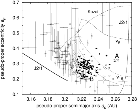
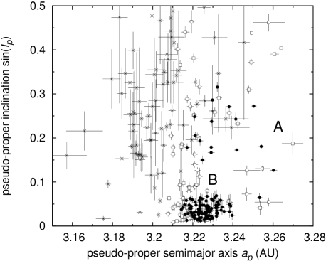
Figure 2: Pseudo-proper orbital elements for the 247 objects in the J2/1 resonance projected onto the planes of semimajor axis $a_{p}$ vs eccentricity $e_{p}$ (top) and semimajor axis $a_{p}$ vs sine of inclination $\sin i_{p}$ (bottom). Bars are standard deviations of the elements derived from 1 Myr numerical integration. Position of several secular resonances embedded in J2/1 is shown in the upper panel. The unstable population of asteroids (crosses) occupies the region of their overlap; the stable population (full circles) occupies two distinct zones –A and B– of low-eccentricity and low-inclination orbits (e.g., Nesvorný & Ferraz-Mello 1997). The population of marginally stable asteroids (open squares) resides in region adjacent to the unstable borders of the resonance or near the bridge over the stable regions associated with the $\nu_{16}$ secular resonance.

The size-frequency distribution of objects of a population is an important property, complementing that of the orbital distribution. Figure 3 shows cumulative distribution $N({<}H)$ of the absolute magnitudes $H$ for bodies in the J2/1 (and other Jovian first order resonances as well). In between $H=12\,{\rm mag}$ and $14.5\,{\rm mag}$ (an approximate completeness limit; R. Jedicke, personal communication) it can be matched by a simple power-law $N({<}H)\propto 10^{\gamma H}$, with $\gamma=(+0.70\pm 0.02)$. We thus confirm that the J2/1 population is steeper than it would correspond to a standard collisionally evolved system (e.g., Dohnanyi 1969; O’Brien & Greenberg 2003) with $\gamma=+0.5$. The same result holds for both the short- and long-lived sub-populations in this resonance separately.

Figure 3: Cumulative distributions $N({<}H)$ of the absolute magnitude $H$ values for population of asteroids in the Jovian first order mean motion resonances: (i) J2/1 (dashed curve), (ii) J3/2 (solid curve), and (iii) J4/3 (dotted curve). The straight lines show best-fit approximations $N({<}H)\propto 10^{\gamma H}$ with the values of $\gamma$ indicated by the corresponding label. The fit matches $N({<}H)$ for $H$ in the interval $(12,15)\,{\rm mag}$ for J2/1 and $(10.5,14.5)\,{\rm mag}$ for J3/2; no such approximation is available for J4/3 where only three objects are currently known. The $H$ values where the straight line approximations level off from the data roughly correspond to the completeness limit of the population (R. Jedicke, personal communication). For sake of a rough comparison, the upper abscissa gives an estimate of sizes for the albedo value $p_{V}=0.05$, average of the outer belt population.

Albedos of J2/1 bodies are not known, except for (1362) Griqua for which Tedesco et al. (2002) give $p_{V}=0.067$. The surroundings main-belt population has an average $p_{V}=0.05$. For sake of simplicity we convert absolute magnitudes to sizes using this averaged value when needed. For instance in Fig. 4 we show a zoom on the long-lived population of objects in the J2/1 resonance with symbol size weighted by the estimated size of the body. We note large objects are located far from each other and they are quite isolated — no small asteroids are in close surroundings. Both these observations suggest that the long-lived J2/1 population does not contain recently-born collisional clusters.

Figure 4: A zoom on the $(a_{p},e_{p})$ and $(a_{p},\sin i_{p})$ plots from Fig. 2 with relative size of the resonant asteroids indicated by size of the crosses. Note the large bodies, some of which are labelled, reside far from each other.

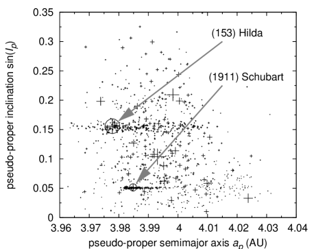
Figure 5: Pseudo-proper orbital elements for 1197 Hildas projected onto the planes of semimajor axis $a_{p}$ vs eccentricity $e_{p}$ (top) and semimajor axis $a_{p}$ vs sine of inclination $\sin i_{p}$ (bottom). Larger size of the symbol indicates larger physical size of the asteroid. Because of Hildas orbital stability, the uncertainty in the pseudo-proper element values is typically smaller than the symbol size. Note a tight cluster around the proper inclination value $\sin i_{p}\simeq 0.0505$, lead by the largest asteroid (1911) Schubart, and a somewhat looser cluster around the proper inclination value $\sin i_{p}\simeq 0.151$, lead by the largest asteroid (153) Hilda. Both are discussed in more detail in Section 3. Solid line denotes the libration centre of the J3/2 resonance.

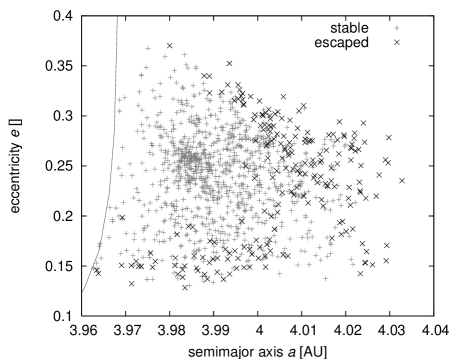
Figure 6: Pseudo-proper semimajor axis vs eccentricity plot for asteroids in the J3/2 resonance. Bold crosses denote orbits, which escaped during the 4 Gyr of evolution. Solid line is the position of the libration centre (the outer separatrix is located further to the right).

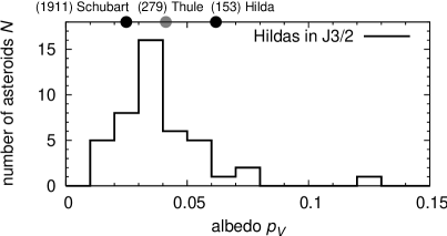
Figure 7: The histogram shows distribution of values of the geometric albedo $p_{V}$ determined by Tedesco et al. (2002) for asteroids located inside the J3/2 resonance. Three individual values – (153) Hilda, (1911) Schubart and (279) Thule (a J4/3 asteroid) – are indicated on top.

2.2 Hilda group

Because asteroids in the J3/2 constitute a rather isolated group, it is easy to select their candidates: we simply extracted from the AstOrb database those asteroids with semimajor axis in between $3.8$ AU and $4.1$ AU. With that we obtained 1267 multi-opposition objects. We numerically integrated these orbits for 10 kyr and analysed the behaviour of the resonance angle $\sigma=3\lambda^{\prime}-2\lambda-\varpi$. We obtained 1197 cases for which $\sigma$ librates about $0^{\circ}$ and which have $N\geq 0.44$, a threshold of the resonance zone (e.g., Morbidelli & Moons 1993); see Fig. 5.

The long-term evolution of Hildas indicates that not all of them are stable over 4 Gyr, but 20 % escape earlier. A brief inspection of Fig. 6 shows, that the escapees are essentially asteroids located closer to the outer separatrix and exhibiting large amplitudes of librations. If the Hilda group has been constituted during the planetary formation some 4 Gyr ago, some non-conservative process must have placed these objects onto their currently unstable orbits. We suspect mutual collisions or gravitational scattering on the largest Hilda members might be the corresponding diffusive mechanisms. Small enough members might be also susceptible to the resonant Yarkovsky effect (see Sec. 4.2 and the Appendix A).

Data in Fig. 3 confirm earlier findings that the Hilda group is characterized by an anomalously shallow size distribution. In between absolute magnitudes $H=10.5\,{\rm mag}$ and $14.5\,{\rm mag}$ the cumulative distribution can be well matched by $N({<}H)\propto 10^{\gamma H}$ with $\gamma=(+0.35\pm 0.02)$ only.

Sub-populations among Hilda asteroids, namely two collisional families, are studied in Section 3.

2.3 Thule group

In spite of a frequent terminology “Thule group”, asteroids in the J4/3 resonance consisted of a single object (279) Thule up to now. Nesvorný & Ferraz-Mello (1997) considered this situation anomalous because the extent of the stable zone of this resonance is not much smaller than that of the J3/2 resonance (see also Franklin et al. 2004). In the same way, our knowledge about the low-$e$ and low-$i$ Thule-type stable orbits (e.g., $a=4.27$ AU, $e=0.1$ and $i=5^{\circ}$) should be observationally complete at about magnitudes $H=12.5\mbox{--}13\,{\rm mag}$ (R. Jedicke, personal communication). A rough estimate also shows that even one magnitude in $H$ beyond this completeness limit the Thule population should be known at $\sim 10$% completeness, leaving only about $90$ % undiscovered population. We thus conclude that the objects in the magnitude range $H=9\mbox{--}13\,{\rm mag}$ are very likely missing in this resonance. Where does the existing population of small Thule-type asteroids begin?

Our initial search in the broad box around the J4/3 resonance detected only 13 objects. Six of them, including the well-known extinct comet (3552) Don Quixote (e.g., Weissman et al. 2002), are on typical orbits of Jupiter-family comets that happen to reside near this resonance with very high eccentricity and moderately high inclination. Two more are single-opposition objects and one has only poorly constrained orbit, leaving us with (279) Thule and three additional candidate objects: (52007) 2002 EQ47, (186024) 2001 QG₂₀₇ and (185290) 2006 UB₂₁₉.

Table 1: Data on presently known population of asteroids residing in the J4/3 Jovian mean motion resonance (Thule group). Pseudo-proper orbital elements $(a_{p},e_{p},\sin i_{p})$ are given together with their standard deviations $(\delta a_{p},\delta e_{p},\delta\sin i_{p})$ determined from a $1$ Myr numerical integration. $\sigma_{p,\,max}$ is the maximum libration amplitude in the Sessin’s $(K,H)$ variables (see Fig. 8), $H$ is the absolute magnitude from the AstOrb catalogue and $D$ is the estimated size using $p_{V}=0.04$ geometric albedo (Tedesco et al. 2002).

No.	Name	$a_{p}$	$e_{p}$	$\sin i_{p}$	$\delta a_{p}$	$\delta e_{p}$	$\delta\sin i_{p}$	$\sigma_{p,\,max}$	$H$	$D$
		[AU]			[AU]			[deg]	[mag]	[km]
279	Thule	4.2855	0.119	0.024	0.0005	0.012	0.003	${\sim}50$	$8.57$	$126.6$
186024	2001 QG207	4.2965	0.244	0.042	0.0003	0.014	0.003	25	$14.36$	$8.9$
185290	2006 UB219	4.2979	0.234	0.102	0.0003	0.014	0.004	25	$13.75$	$11.8$

Figure 8: Top panels: orbits of (279) Thule [left], (186024) 2001 QG₂₀₇ [middle] and (185290) 2006 UB₂₁₉ [right] in resonant variables $(e\cos\sigma,e\sin\sigma)$ of the J4/3 resonance. Here $e$ is the eccentricity and $\sigma=4\lambda^{\prime}-3\lambda-\varpi$, with $\lambda$ and $\lambda^{\prime}$ the mean longitude in orbit of the asteroid and Jupiter and $\varpi$ is the longitude of asteroid’s pericentre (in all cases the osculating orbital elements are used). Each panel shows results of a short-term, 10 kyr numerical integration. In all three cases the orbits librate about the pericentric branch ($\sigma=0^{\circ}$) of the resonance. Perturbations due to Jupiter’s eccentricity and its variations make the regular libration move in an epicyclic manner (e.g., Ferraz-Mello 1988; Sessin & Brassane 1988). Bottom panels: filtered resonant variables $(e\cos\sigma,e\sin\sigma)$, with short-period oscillations forced by Jupiter removed by digital filtering. They are similar to Sessin’s $(K,H)$ coordinates in Sessin & Brassane (1988) or Tsuchida (1990). In each of the cases the pericentric libration is clearly revealed. The maximum libration amplitude in these coordinates is denoted by $\sigma_{p,\,max}$ in Table 1.

Figure 8 (top panels) shows short-term tracks of (279) Thule, (186024) 2001 QG₂₀₇ and (185290) 2006 UB₂₁₉ in resonant variables $\sqrt{2\Sigma}\,(\cos\sigma,\sin\sigma)\simeq(e\cos\sigma,e\sin\sigma)$ of the J4/3 resonance ($\sigma=4\lambda^{\prime}-3\lambda-\varpi$ in this case). In all cases their orbits librate about the pericentric branch ($\sigma=0^{\circ}$) of this resonance, although this is complicated –mainly in the low-eccentricity case of (279) Thule– by the forced terms due to Jupiter’s eccentricity (see, e.g., Ferraz-Mello 1988; Sessin & Bressane 1988; Tsuchida 1990). The leftmost panel recovers the $40^{\circ}\mbox{--}50^{\circ}$ libration of (279) Thule, determined previously by Tsuchida (1990; Fig. 3). The other two smaller asteroids show librations with comparable amplitudes. The last object, (52007) 2002 EQ47, appears to reside on an unstable orbit outside the J4/3 resonance. Our search thus lead to the detection of two new asteroids in this resonance, increasing its population by a factor of three.

Results of a long-term numerical integration of the nominal orbits plus 10 close clones, placed within an orbital uncertainty, reveal that the orbit of (279) Thule is stable over 4 Gyr, but the orbits of (186024) 2001 QG₂₀₇ and (185290) 2006 UB₂₁₉ are partially unstable. They are not ‘short-lived’ but 45 % and 60 % of clones, respectively, escaped before 4 Gyr. Figure 9 shows pseudo-proper semimajor axis vs time for nominal orbits and their clones of all J4/3 objects; the escaping orbits leave the figure before the simulation was ended at 4 Gyr. We suspect similar non-conservative effects as mentioned above for the 20% fraction of long-term-unstable Hildas to bring these two Thule members onto their marginally stable orbits.

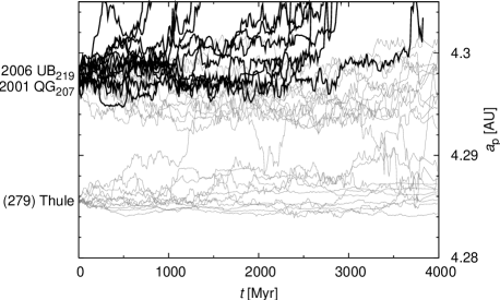
Figure 9: Pseudo-proper semimajor axis $a_{\rm p}$ vs time $t$ plot for the 3 orbits of asteroids located inside the J4/3 resonance and 10 close clones orbits (placed randomly within the uncertainty ellipsoids) for each of them. Thin lines denote the stable orbits and thick lines unstable, which escaped from the J4/3 before the completion of the simulation at 4 Gyr.

We would like to point out that it took more than a century from the discovery of (279) Thule (Palisa 1888; Krueger 1889) until further objects in this resonance were finally discovered. This is because there is an anomalously large gap in size of these bodies: (279) Thule is $127$ km in size with $p_{V}=0.04$ AU (e.g., Tedesco et al. 2002), while the estimated sizes of (186024) 2001 QG₂₀₇ and (185290) 2006 UB₂₁₉ for the same value of albedo are $8.9$ km and $11.8$ km only. It will be interesting to learn as much as possible about the Thule population in the $H=13\mbox{--}15$ mag absolute magnitude range using future-generation survey projects such as Pan-STARRS (e.g., Jedicke et al. 2007). Such a completed population may present an interesting constraint on the planetesimal size distribution 4 Gyr ago.

3 Collisional families among Hilda asteroids

Collisions and subsequent fragmentations are ubiquitous processes since planets formed in the Solar system. Because the characteristic dispersal velocities of the ejecta (as a rule of thumb equal to the escape velocity of the parent body) are usually smaller than the orbital velocity, the resulting fragments initially reside on nearby orbits. If the orbital chaoticity is not prohibitively large in the formation zone, we can recognise the outcome of such past fragmentations as distinct clusters in the space of sufficiently stable orbital elements. More than 30 collisional families are known and studied in the main asteroid belt (e.g., Zappalà et al. 2002) with important additions in the recent years (e.g., Nesvorný et al. 2002; Nesvorný, Vokrouhlický & Bottke 2006). Similarly, collisional families have been found among the Trojan clouds of Jupiter (e.g., Milani 1993; Beaugé & Roig 2001; Roig et al. 2008), irregular satellites of Jupiter (e.g., Nesvorný et al. 2003, 2004) and even trans-Neptunian objects (e.g., Brown et al. 2007). Mean motion resonances, other than the Trojan librators of Jupiter, are typically too chaotic to hold stable asteroid populations, or the populations were too small to enable search for families. The only remaining candidate populations are those in the Jovian first order resonances, with Hilda asteroids the most promising group. However, low expectations for an existence of collisional families likely de-motivated systematic search. Note, the estimated intrinsic collisional probability of Hilda asteroids is about a factor 3 smaller than in the main asteroid belt (e.g., Dahlgren 1998; Dell’Oro et al. 2001) and the population is more than two orders of magnitude smaller.

In spite of the situation outlined above, Schubart (1982a, 1991) repeatedly noticed groups of Hilda-type asteroids with very similar proper elements. For instance, in his 1991 paper he lists 5 members of what we call Schubart family below and pointed out their nearly identical values of the proper inclination. Already in his 1982 paper Schubart mentions a similarity of such clusters to Hirayama families, but later never got back to the topic to investigate this problem with sufficient amount of data provided by the growing knowledge about the J3/2 population. Even a zero order inspection of Fig. 5, in particular the bottom panel, implies the existence of two large clusters among the J3/2 population. In what follows we pay a closer analysis to both of them.

We adopt an approach similar to the hierarchical-clustering method (HCM) frequently used for identification of the asteroid families in the main belt (e.g., Zappalà et al. 1990, 1994, 2002). In the first step of our analysis, we compute the number of bodies $N_{\rm min}$ which is assumed to constitute a statistically significant cluster for a given value of the cutoff velocity $v_{\rm cutoff}$. We use a similar approach to that of Beaugé & Roig (2001): for all asteroids in the J3/2 resonance we determine the number $N_{i}(v_{\rm cutoff})$ of asteroids which are closer than $v_{\rm cutoff}$. Then we compute the average value $N_{0}=\bar{N}_{i}$. According to Zappalà et al. (1994), a cluster may be considered significant if $N>N_{\rm min}=N_{0}+2\sqrt{N_{0}}$. The plots $N_{0}(v_{\rm cutoff})$ and the corresponding $N_{\rm min}(v_{\rm cutoff})$ for Hilda population are shown in Fig. 10. We use a standard metric ($d_{1}$ defined by Zappalà et al., 1994), namely:

$$\delta v=na_{p}\sqrt{{5\over 4}\left({\delta a_{p}\over a_{p}}\right)^{2}+2\,(\delta e_{p})^{2}+2\,(\delta\sin i_{p})^{2}}\;,$$ (8)

where $(a_{p},e_{p},\sin i_{p})$ are 10 Myr averaged values of the resonant pseudo-proper elements (we checked that our results practically do not depend on the width of this averaging interval).

Figure 10: The dependence of the minimum number of asteroids $N_{\rm min}$, to be considered a statistically significant cluster, on the cutoff velocity $v_{\rm cutoff}$ (thick curve). The average number $N_{0}$ and the maximum number ${\rm max}(N_{i})$ of asteroids, which are closer than $v_{\rm cutoff}$, is shown by dashed and thin curves. All quantities are valid for the J3/2 population. The fact that ${\rm max}(N_{i})$ is much larger than $N_{0}$ and $N_{\rm min}$ indicates a presence of a significant cluster (or clusters) among the Hilda group.

Next, we construct a stalactite diagram for Hildas in a traditional way (e.g., Zappalà et al. 1990): we start with (153) Hilda as the first central body and we find all bodies associated with it at $v_{\rm cutoff}=300\,{\rm m}/{\rm s}$, using a hierarchical clustering method (HCM; Zappalà et al. 1990, 1994). Then we select the asteroid with the lowest number (catalogue designation) from remaining (not associated) asteroids and repeat the HCM association again and again, until no asteroids are left. Then we repeat the whole procedure recursively for all clusters detected at $v_{\rm cutoff}=300\,{\rm m}/{\rm s}$, but now for a lower value, e.g., $v_{\rm cutoff}=299\,{\rm m}/{\rm s}$. We may continue until $v_{\rm cutoff}=0\,{\rm m}/{\rm s}$, but of course, for too low values of the cutoff velocity, no clusters can be detected and all asteroids are single. The resulting stalactite diagram at Fig. 11 is simply the asteroid number (designation) vs $v_{\rm cutoff}$ plot: a dot at a given place is plotted only if the asteroids belongs to a cluster of at least ${\rm max}(5,N_{\rm min}(v_{\rm cutoff}))$ bodies. We are not interested in clusters with less than 5 members; they are most probably random flukes.

We can see two prominent clusters among Hildas: the first one around the asteroid (153) Hilda itself, and the second one around (1911) Schubart. In the remaining part of this Section we discuss each of them separately.

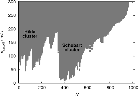
Figure 11: A stalactite diagram computed for the J3/2 population (Hildas). Two prominent groupings, the Schubart family and the Hilda family, are indicated. Every group plotted here has at least 5 or $N_{\rm min}$ members, whichever is larger (see Fig. 10).

The stalactite diagram constructed in the same way for Zhongguos and Griquas is shown in Fig. 12. No grouping seem to be significant enough to be considered an impact-generated cluster. This is consistent with the discussion of the $(a_{p},e_{p},\sin i_{p})$ plots in Section 2.1.

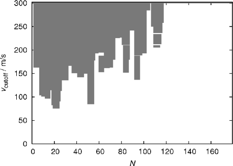
Figure 12: A stalactite diagram computed for the long-lived J2/1 population. There are no prominent groupings; 60 asteroids are not associated with any others, even at $v_{\rm cutoff\/}=300\,{\rm m}/{\rm s}$. Every group plotted here has at least 5 members.

3.1 Schubart family

The Schubart family can be distinguished from the remaining population of Hildas on a large range of cutoff velocities: from 50 m/s to more than 100 m/s (Fig. 11). It merges with the Hilda family at 200 m/s. For the purpose of our analysis we selected $v_{\rm cutoff}=60\,{\rm m}/{\rm s}$ as the nominal value. While the total number of Schubart family members is not too sensitive to this cutoff value, we refrain from using too high $v_{\rm cutoff}$, for which we would expect and increasing number of interlopers to be associated with the family, and the family would attain a rather peculiar shape in the $(a_{p},e_{p},\sin i_{p})$ space.

Figure 13 shows the cumulative distribution of the absolute magnitudes for the Schubart family members, compared to the rest of the J3/2 population. Importantly, the slope $\gamma=(+0.48\pm 0.02)$ of the $N({<}H)\propto 10^{\gamma H}$ fit is quite steeper for the Schubart family, which supports the hypothesis of its collisional origin.

Figure 13: Cumulative distributions $N({<}H)$ of absolute magnitudes $H$ for the whole J3/2 population (solid) and for the members of the families around (153) Hilda (dashed) and (1911) Schubart (dotted). Thin dotted curves denote $N({<}H)$ of the J3/2 population with one and both families subtracted. Labels are the best-fitted values of $\gamma$ using $N({<}H)\propto 10^{\gamma H}$ (straight lines) in the interval $(12.25,14.25)$ for Hilda and $(12.25,14.75)$ for Schubart clusters. For sake of a rough comparison, the upper abscissa gives an estimate of the sizes for an albedo value $p_{V}=0.044$, average of the J3/2 population.

We also analysed the available SDSS catalogue of moving objects (ADR3; Ivezić et al. 2002). We searched for the J3/2 asteroids among the entries of this catalogue and computed the principal component PC₁ of the spectrum in the visible band. Note the PC₁ value is an indicator of the spectral slope and allows thus to broadly distinguish principal spectral classes of asteroids (e.g., Bus et al. 2002). Figure 14 shows our results. The top panel confirms the bimodal character of the J3/2 population (see also Dahlgren et al. 1997, 1998, 1999 and Gil-Hutton & Brunini 2008). More importantly, though, the bottom panel indicates a spectral homogeneity of the Schubart family, placing all members within the C/X taxonomy class branch. This finding strongly supports collisional origin of the Schubart family.

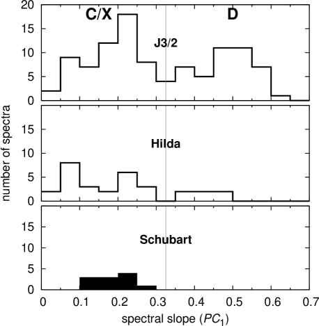
Figure 14: Distribution of spectral slopes (PC₁ components of the 5 broad-band colours) of 153 asteroids in the J3/2 resonance (top), 21 Hilda family members (middle) and 4 Schubart family members (bottom). Data computed from the 3rd release of the SDSS catalogue of moving objects (ADR3; Ivezić et al. 2002). Note some objects have been observed multiple times by SDSS and the histograms show distribution of all observations (rather than averages for a given body). The slope values of Hildas range from neutral to steep, with roughly two groups separated by the value PC${}_{1}=0.3$: (i) C/X-types with PC${}_{1}<0.3$, and (ii) D-types with PC${}_{1}>0.3$. Importantly, the Schubart family members are spectrally similar; the median value PC${}_{1}=0.20$ corresponds to a C- or X-type parent body.

Tedesco et al. (2002) derive $D=80$ km size for (1911) Schubart, corresponding to a very low albedo $p_{V}=0.025$. The same authors determine $D=38$ km size of (4230) van den Bergh and exactly the same albedo; this asteroid is among the five largest in the family. Assuming the same albedo for all other family members, we can construct a size-frequency distribution (Fig. 15). The slope $\alpha\simeq(-2.7\pm 0.1)$ fitted to the small end of the distribution, where we still assume observational completeness, is rather shallow, but marginally within the limits of population slopes produced in the numerical simulations of disruptions (e.g., Durda et al. 2007).

Figure 15: Cumulative size distribution $N({>}D)$ for the whole J3/2 population (solid) and for members of the two suggested collisional clusters: Hilda (dashed) and Schubart (dotted). We assumed the geometric albedo $p_{V}=0.044$ (and $0.025$ in the Schubart-family case; see the text) for the conversion of absolute magnitudes $H$ to diameters $D$. Labels are the best-fitted values of $\alpha$ using $N({>}D)\propto D^{\alpha}$ (straight lines) in the interval $(11,20)$ km for the two families and $(9,20)$ km for the J3/2 population.

If we sum the volumes of the observed members, we end up with a lower limit for the parent body size $D_{\rm PB}=110\,{\rm km}$, provided there are no interlopers. We can also estimate the contribution of small (unobserved) bodies using the following simple method: (i) we sum only the volumes of the observed bodies larger than an assumed completeness limit $D_{\rm complete}=10\,{\rm km}$ ($V_{\rm complete}=\sum_{i}{\pi\over 6}D_{i}^{3}$); (ii) we fit the cumulative size distribution by a power law ($\log N({>}D)=\alpha\log[D]_{\rm km}+\beta$; $\alpha=-2.68$, $\beta=4.73$ for the Schubart); (iii) we prolong this slope from $D_{\rm complete}$ down to $D_{\rm min}=0$ and calculate the total volume of the parent body (provided $\alpha>-3$):

$$V_{\rm PB}=V_{\rm complete}+{\pi\over 6}10^{\beta}{\alpha\over\alpha+3}\left[D_{\rm min}^{a+3}-D_{\rm complete}^{a+3}\right]\;.$$ (9)

The result is $D_{\rm PB}=\sqrt[3]{{6\over\pi}V_{\rm PB}}\doteq 130\,{\rm km}$, some sort of an upper limit. The volumetric ratio between the largest fragment and the parent body is then $V_{\rm LF}/V_{\rm PB}\doteq 0.2$, a fairly typical value for asteroid families in the main asteroid belt. Obviously, the assumption of a single power-law extrapolation of the $N({>}D)$ at small sizes is only approximate and can lead to a result with a $10$ % uncertainty. However, if we use an entirely different geometric method, developed by Tanga et al. (1998), we obtain $D_{\rm PB}\simeq 120\mbox{--}130$ km, i.e., comparable to our previous estimate.

What is an approximate size $d_{\rm disrupt}$ of a projectile necessary to disrupt the parent body of the Schubart family? Using Eq. (1) from Bottke et al. (2005):

$$d_{\rm disrupt}=\left(2Q_{D}^{*}/V_{\rm imp}^{2}\right)^{1\over 3}D_{\rm target}\;.$$ (10)

and substituting $Q_{D}^{*}=10^{5}\,{\rm J}/{\rm kg}$ for the strength (somewhat lower than that of basaltic objects to accommodate the assumed C/X spectral type; e.g., Kenyon et al. 2008 and references therein), $V_{\rm imp}=4.78\,{\rm km}/{\rm s}$ for the typical impact velocity (see Dahlgren 1998) and $D_{\rm target}\simeq 130\,{\rm km}$, we obtain $d_{\rm disrupt}\simeq 25\,{\rm km}$. At this size the projectile population is dominated by main belt bodies. Considering also different intrinsic collisional probabilities between Hilda–Hilda asteroids ($2.3\times 10^{-18}\,{\rm km}^{-2}\,{\rm yr}^{-1}$; Dahlgren 1998) and Hilda–main belt asteroids ($0.6\times 10^{-18}\,{\rm km}^{-2}\,{\rm yr}^{-1}$), we find it more likely the Schubart family parent body was hit by a projectile originating from the main belt.

3.2 Hilda family

We repeated the same analysis as in Section 3.1 for the Hilda family. The family remains statistically distinct from the whole J3/2 population in the range of cutoff velocities $(130,170)\,{\rm m}/{\rm s}$; we choose $v_{\rm cutoff}=150\,{\rm m}/{\rm s}$ as the nominal value.

The slope $\gamma$ of the cumulative absolute magnitude distribution $N({<}H)$ is $(+0.50\pm 0.02)$ (Fig. 13), again steeper than for the total J3/2 population and comparable to that of the Schubart family. The spectral slopes (PC₁) are somewhat spread from flat (C/X-compatible values; PC${}_{1}<0.3$) to redder (D-compatible values; PC${}_{1}>0.3$) — see Fig. 14. Overall, though, the C/X members prevail such that the D-type objects might be actually interlopers, at least according to a simple estimate based on the volume of the Hilda family in the $(a_{p},e_{p},\sin i_{p})$ space, compared to the total volume of the J3/2 population.

Tedesco et al. (2002) determine albedos for six family members. They range from 0.037 to 0.087, but three values are close to the median albedo 0.044 of all J3/2 asteroids. We thus consider this value to be representative of the Hilda family. The corresponding cumulative size distribution is plotted in Fig. 15. Using the same method as in Section 3.1 we estimate the size of the parent body $D_{\rm PB}=180\mbox{--}190\,{\rm km}$, with $V_{\rm LF}/V_{\rm PB}\simeq 0.8$. With the model of Tanga et al. (1999) we would obtain $D_{\rm PB}\simeq 210$ km and thus $V_{\rm LF}/V_{\rm PB}\simeq 0.5$. This family forming event seems to be thus characterized in between the catastrophic disruption and a huge cratering. The necessary projectile size is $d_{\rm disrupt}=50\mbox{--}55$ km.

While not so prominent as the Schubart family, we consider the group of asteroids around Hilda a fairly robust case of a collisionally-born family too.

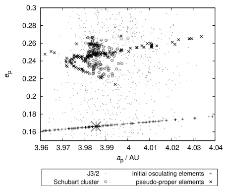
Figure 16: The initial osculating elements of an impact-generated swarm of 139 fragments at the location of (1911) Schubart (bottom crosses), the corresponding pseudo-proper elements computed from the first My of evolution (upper crosses) and the pseudo-proper elements of the observed Schubart family (circles). We show here projection onto the plane defined by semimajor axis and eccentricity. Dots are the pseudo-proper elements of the background J3/2-population asteroids. The initial synthetic swarm of asteroids poorly matches the observed family: it is both too extent in semimajor axis and too compact in eccentricity.

Figure 17: The same as Fig. 16, but for a different impact geometry ($f=135^{\circ}$, $\omega+f=180^{\circ}$). This choice of $f$ maximizes the initial spread of the synthetic family in proper eccentricity. In this case we do not show the initial osculating orbital elements.

3.3 Simulated disruption events

In order to asses some limits for the age of the Schubart and Hilda families, we perform a number of numerical tests. In particular, we simulate a disruption of a parent body inside the resonance and numerically determine the long-term orbital evolution of fragments. The evolved synthetic family at different time steps is then compared with the observed family. Ideally, this approach should allow to constrain the time elapsed since the family formed.

As a first step, we need to create a synthetic family inside the resonance. We use current orbital elements of the largest family member, (1911) Schubart in this case, as representative to the parent body and only allow changes in the true anomaly $f$ and in the argument of pericentre $\omega$ at the break-up event. By changing these two geometric parameters we can produce different initial positions of the fragments in the orbital element space. For sake of our test, fragments are assumed to be dispersed isotropically with respect to the parent body, with a velocity distribution given by the model of Farinella et al. (1993, 1994). The number of fragments $dN(v)$ launched with relative velocities in the interval $(v,v+dv)$ is given by

$$dN(v)=Cv(v^{2}+v_{\rm esc}^{2})^{-(\kappa+1)/2}\,dv\;,$$ (11)

with $C$ a normalization constant, $v_{\rm esc}$ the escape velocity from the parent body and $\kappa=3.25$. To prevent excessive escape velocities we introduce a maximum allowed value $v_{\rm max}$. Nominally, we set $v_{\rm max}=200$ m/s, but in the next Section 3.4 we also use restricted values of this parameter to test sensitivity of our results to initial conditions.

To simulate an impact that might have created the Schubart family, we generated velocities randomly for 139 fragments with $v_{\rm esc}=65\,{\rm m}/{\rm s}$ (note the number of fragments in the synthetic family is equal to the number of the Schubart family members). The resulting swarm of fragments is shown in Fig. 16, for the impact geometry $f=0^{\circ}$ and $\omega+f=180^{\circ}$. We show both the initial osculating orbital elements and the pseudo-proper elements.

The synthetic family extends over significantly larger range of the semimajor axis than the observed Schubart family, but all fragments still fall within the J3/2 resonance. The eccentricity distribution is, on the other hand, substantially more compact. Only the distribution of inclinations of the synthetic family roughly matches that of the observed family. We verified this holds also for other isotropic-impact geometries (such as $f=135^{\circ}$ and $\omega+f=180^{\circ}$ shown in Fig. 17). The peculiar shape of the synthetic family in the pseudo-proper element space $(a_{p},e_{p})$ is an outcome of the isotropic disruption, simply because some fragments fall to the left from the libration centre of the J3/2 resonance (at 3.97 AU) and they are ‘mapped’ to the right. This is because the pseudo-proper elements are the maxima and minima of $a$ and $e$, respectively, over their resonant oscillations.

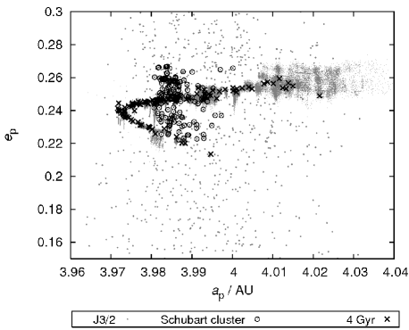
Figure 18: The synthetic family from Fig. 16 evolved over 4 Gyr: the grey dots show evolutionary tracks of the fragments in the pseudo-proper orbital element space. Overall, stability of the J3/2 resonance makes many fragments to stay very close to their initial values. Only ${\sim}10\,\%$ of fragments with the initial extremal values of $a_{p}$ (and thus the libration amplitude) escape from the resonance during the simulation. This helps in part to reduce the mismatch with the observed family (circles) in semimajor axis, but is not sufficient to attain the Schubart-family full eccentricity dispersion.

The initial configuration of the synthetic family was propagated for 4 Gyr, using the integrator described in Section 2. At this stage, we use only the gravitational perturbations from the 4 exterior giant planets. We performed such simulation for several impact geometries, as determined by $f$ and $\omega$, with similar results.

Figure 18 shows the long-term evolution of the synthetic family. Because the family resides mostly in the stable zone of the J3/2 resonance, only little evolution can be seen for most of the bodies. This is in accord with findings of Nesvorný & Ferraz-Mello (1997) who concluded that the stable region in this resonance shows little or no diffusion over time scales comparable to the age of the Solar system. Only about $10$ % of orbits that initially started at the outskirts of the stable zone (with large libration amplitudes) escaped from the resonance during the 4 Gyr simulation.

The removal of orbits with large semimajor axis $a_{p}$ helps in part to reconcile the mismatch with the distribution of the observed Schubart family. However, the dispersion in eccentricity $e_{p}$ does not evolve much and it still shows large mismatch if compared to the observed family. Even in the case $f=135^{\circ}$ ($\omega+f=180^{\circ}$; Fig. 17), which maximizes the initial eccentricity dispersion of the synthetic fragments, the final value at 4 Gyr is about three times smaller than that of the Schubart family. Clearly, our model is missing a key element to reproduce the current orbital configuration of this family.

One possibility to resolve the problem could be to release the assumption of an isotropic impact and explore anisotropies in the initial velocity field. This is an obvious suspect in all attempts to reconstruct orbital configurations of the asteroid families, but we doubt it might help much in this case. Exceedingly large relative velocities, compared to the escape velocity of the estimated parent body, would be required. Recall, the fragments located in the stable region of the J3/2 resonance would hardly evolve over the age of the Solar system.

A more radical solution is to complement the force model, used for the long-term propagation, by additional effects. The only viable mechanism for the size range we are dealing with is the Yarkovsky effect. This tiny force, due to anisotropic thermal emission, has been proved to have determining role in understanding fine structures of the asteroid families in the main belt (e.g., Bottke et al. 2001; Vokrouhlický et al. 2006a,b). In these applications the Yarkovsky effect produces a steady drift of the semimajor axis, leaving other orbital elements basically constant.

However, the situation is different for resonant orbits. The semimajor axis evolution is locked by the strong gravitational influence of Jupiter. For that reason we first ran simplified simulations with the Yarkovsky forces — results of these tests are briefly described in the Appendix A. We next applied the model containing both gravitational and Yarkovsky perturbations to the evolution of the synthetic family. Results of these experiments are described in the next Section 3.4.

3.4 Yarkovsky drift in eccentricity

We ran our previous simulation of the long-term evolution of the synthetic family with the Yarkovsky forces included. Our best guess of thermal parameters for bodies of the C/X type is: $\rho_{\rm s}=\rho_{\rm b}=1300\,{\rm kg}/{\rm m}^{3}$ for the surface and bulk densities, $K=0.01\,{\rm W}/{\rm m}/{\rm K}$ for the surface thermal conductivity, $C=680\,{\rm J}/{\rm kg}$ for the heat capacity, $A=0.02$ for the Bond albedo and $\epsilon=0.95$ for the thermal emissivity parameter. Rotation periods are bound in the 2–12 hours range. Spin axes orientations are assumed isotropic in space. Finally, we assign sizes to our test particles equal to the estimate of sizes for Schubart family members, based on their reported absolute magnitudes and albedo $p_{V}=0.025$. The dependence of the Yarkovsky force on these parameters is described, e.g., in Bottke et al. (2002, 2006). We note the uncertainties of the thermal parameters, assigned to individual bodies, do not affect our results significantly, mainly because we simulate a collective evolution of more than 100 bodies; we are not interested in evolution of individual orbits.

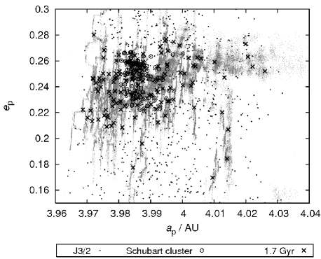
Figure 19: The impact-generated swarm from Fig. 16 evolved by planetary perturbations and the Yarkovsky forces, in the projection on the pseudo-proper semimajor axis $a_{p}$ vs eccentricity $e_{p}$ plane. The grey dots indicate the evolutionary tracks over the whole 4 Gyr time span and crosses denote the configuration at 1.7 Gyr, when the eccentricity dispersion of the synthetic family particles roughly matches that of the observed Schubart family (circles).

We let the synthetic family evolve for 4 Gyr and recorded its snapshots every 50 kyr. As discussed in the Appendix A, the resonant Yarkovsky effect produces mainly secular changes of eccentricity. We recall this systematic drift in $e$ must not be confused with the chaotic diffusion in $e$. We also note that inclination of the orbits remains stable, in accord with a good match of the Schubart family by the initial inclination distribution.

Because the initial eccentricity dispersion of the synthetic family is much smaller than that of the observed one, its steady increase due to the combined effects of the Yarkovsky forces and the resonant lock gives us a possibility to date the origin of the family (see Vokrouhlický et al. 2006a for a similar method applied to families in the main belt). To proceed in a quantitative way, we use a 1-dimensional Kolmogorov–Smirnov (KS) test to compare cumulative distribution of pseudo-proper eccentricity values $e_{p}$ of the observed and synthetic families (e.g., Press et al. 2007).

Figure 20 shows the KS distance $D_{KS}$ of the two eccentricity distributions as a function of time. For sake of a test, we also use smaller $v_{\rm max}$ values of the initial velocity field (essentially, this is like to start with a more compact synthetic family). Regardless of the $v_{\rm max}$ value, our model rejects Schubart family ages smaller than 1 Gyr and larger than 2.4 Gyr with a 99 % confidence level. For ages in between 1.5 Gyr and 1.7 Gyr the KS-tested likelihood of a similarity of the synthetic-family and the observed-family $e_{p}$ distributions can reach up to $50$ %. We thus conclude the most likely age of the Schubart cluster is $(1.7\pm 0.7)\,{\rm Gyr}$.

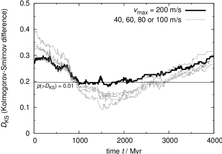
Figure 20: The difference between the cumulative distribution of eccentricities for the observed Schubart family and our synthetic families expressed as the Kolmogorov–Smirnov (KS) distance $D_{\rm KS}$ vs time $t$. All models assume $f=0^{\circ}$ and $\omega+f=180^{\circ}$ but they have different maximum values $v_{\rm max}$ of the ejected particles: $v_{\rm max}=40$, 60, 80, 100 and 200 m/s (labels). For $t<1\,{\rm Gyr}$ and $t>2.4\,{\rm Gyr}$ the KS distance is large such that the KS probability is $p({>}D_{\rm KS})<0.01$. Thus with a 99% probability level we can exclude such age for the Schubart family. The best matches are achieved for $v_{\rm max}=40$ and 60 m/s, for which the most extreme particles have been eliminated from the synthetic family.

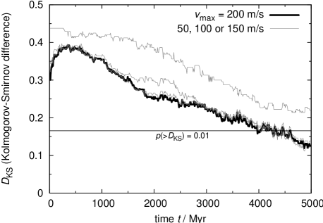
Figure 21: The same as Fig. 20 but for the Hilda family. The KS distance $D_{\rm KS}$ of the observed and modelled pseudo-proper eccentricity $e_{p}$ distribution for several synthetic clusters with different maximum velocities $v_{\rm max}$ are plotted vs time $t$. In this case, $t\leq 3.5$ Gyr seems to be ruled out at a 99 % probability level.

We repeated the same analysis for Hilda family by creating a synthetic family of 233 particles about (153) Hilda. In this case we used $v_{\rm esc}=110\,{\rm m}/{\rm s}$. The situation is actually very similar to the Schubart — there is again a problem with the small dispersion of eccentricities in case of a purely gravitational model. Using the model with the Yarkovsky effect, we can eventually fit the spread of eccentricities and according to the KS test (Fig. 21) the age of the family might be $\gtrsim 4$ Gyr. The match is still not perfect, but this problem might be partly due to numerous interlopers in the family. We also note that a 10 % relative uncertainty of the mean albedo of the Hilda family members would lead to a 5 % uncertainty of their sizes and, consequently, to a 5 % uncertainty of the family age.

The Hilda family seems to be dated back to the Late Heavy Bombardment era (Morbidelli et al. 2005; see also Sec. 4.1). We would find such solution satisfactory, because the population of putative projectiles was substantially more numerous than today (note that a disruption of the Hilda family parent body is a very unlikely event during the last 3.5 Gyr).

We finally simulated a putative collision in the J2/1 resonance, around the asteroid (3789) Zhongguo (the largest asteroid in the stable island B). There are two major differences as compared to the J3/2 resonance: (i) the underlying chaotic diffusion due to the gravitational perturbations is larger in the J2/1 resonance (e.g., Nesvorný & Ferraz-Mello 1997), such that an initially compact cluster would fill the whole stable region in 1–1.5 Gyr and consequently becomes unobservable; (ii) sizes of the observed asteroids are generally smaller, which together with a slightly smaller heliocentric distance, accelerates the Yarkovsky drift in $e_{p}$. The latter effect would likely shorten the time scale to 0.5–1 Gyr. Thus the non-existence of any significant orbital clusters in the J2/1 resonance (Sec. 3 and Fig. 12) does not exclude a collisional origin of the long-lived population by an event older than 1 Gyr. This would also solve the apparent problem of the very steep size distribution of the stable J2/1 population (Brož et al. 2005 and Fig. 3). Note the expected collisional lifetime of the smallest observed J2/1 asteroids is several Gyr (e.g., Bottke et al. 2005).

4 Resonant population stability with respect to planetary migration and the Yarkovsky effect

We finally pay a brief attention to the overall stability of asteroid populations in the first-order resonances with respect to different configurations of giant planets. We are focusing on the situations when the orbits of Jupiter and Saturn become resonant. This is motivated by currently adopted views about final stages of building planetary orbits architecture, namely planet migration in a diluted planetesimal disk (e.g., Malhotra 1995; Hahn & Malhotra 1999; Tsiganis et al. 2005; Morbidelli et al. 2005; Gomes et al. 2005 – these last three references are usually described as the Nice model). Morbidelli et al. (2005) proved that the primordial Trojan asteroids were destabilized when Jupiter and Saturn crossed their mutual 1:2 mean motion resonance and, at the same time, the Trojan region was re-populated by particles of the planetesimal disk. Since the mutual 1:2 resonance of Jupiter and Saturn plays a central role in the Nice model, and since these two planets had to cross other (weaker) mutual resonances such as 4:9 and 3:7 before they acquired today’s orbits, one can naturally pose a question about the stability of primordial populations in the first-order mean motion resonances with Jupiter. Ferraz-Mello et al. (1998a,b) demonstrated that even subtler effects can influence the J2/1 population, namely the resonances between the asteroid libration period in the J2/1 resonance and the period of the Great Inequality (GI) terms in planetary perturbations (i.e., those associated with Jupiter and Saturn proximity to their mutual 2:5 mean motion resonance; Fig. 22). A first glimpse to the stability of the first-order resonance populations with respect to these effects is given in Section 4.1.

In Section 4.2 we also briefly estimate the change of dynamical lifetimes for small J2/1 and J3/2 bodies caused by the Yarkovsky effect.

Figure 22: Dependence of the period associated with circulation of the Great Inequality (GI) angle $5\lambda_{\rm S}-2\lambda_{\rm J}$ ($\lambda_{\rm S}$ and $\lambda_{\rm J}$ are mean longitude in orbit for Saturn and Jupiter) on the osculating semimajor axis $a_{\rm S}$ of Saturn (crosses); Jupiter’s orbit is fixed. Moving Saturn farther away from the location of 2:5 resonance with Jupiter (at $a_{\rm S}=9.584\,{\rm AU}$) makes the GI period shorter (with today’s $a_{\rm S}=9.5289\,{\rm AU}$ the GI period is about 880 yr). In the interval of $a_{\rm S}$ values shown in this figure the GI period becomes comparable to the average period $\bar{P}_{\rm J2/1}$ of librations in the J2/1 resonance (solid line). Libration period for a particular case of asteroid (1362) Griqua is shown by circles.

4.1 Planetary migration effects

In what follows we use a simple approach by only moving Saturn’s orbit into different resonance configurations with Jupiter’s orbit. We do not let orbits of these planets migrate, but consider them static. With such a crude approach we can only get a first hint about a relative role of depletion of the asteroid populations in the first-order resonances (note in reality the planets undergo steady, but likely not smooth, migration and exhibit jumps over different mutual resonant states; e.g., supplementary materials of Tsiganis et al. 2005).

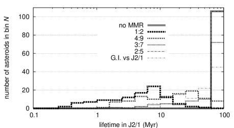
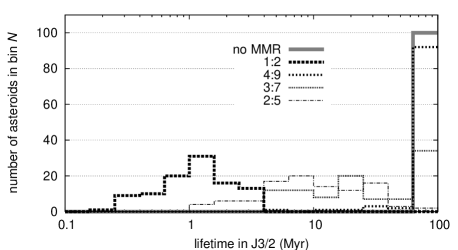
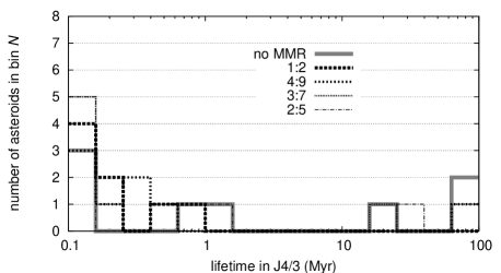
Figure 23: Histograms of dynamical lifetimes for asteroids in the J2/1 [top], J3/2 [middle] and J4/3 [bottom] resonances, in case Jupiter and Saturn are at their current orbits, or in a mutual 1:2, 4:9, 3:7, 2:5 resonance, or in a Great Inequality resonance (in case of the J2/1 only). The histograms were computed for 106 long-lived asteroids in the J2/1, first 100 Hildas in the J3/2 and 8 in the J4/3 (including short-lived).

The results are summarised in Fig. 23. (i) The Hilda group in the J3/2 resonance is very unstable (on the time scale $\sim\!1\,{\rm Myr}$) with respect to the 1:2 Jupiter–Saturn resonance; on the contrary J2/1 asteroids may survive several 10 Myr in this configuration of Jupiter and Saturn, so this population is not much affected by this phase by planetary evolution (note, moreover, that Jupiter and Saturn would likely cross the zone of other mutual 1:2 resonance in $\sim\!1\,{\rm Myr}$ only; e.g., Tsiganis et al. 2005 and Morbidelli et al. 2005). (ii) The 4:9 resonance has a larger influence on the J2/1 population than on Hildas. (iii) In the case of 3:7 resonance it is the opposite: the J3/2 is more unstable than the J2/1. (iv) The Great Inequality resonance does indeed destabilise the J2/1 on a time scale 50 Myr. Provided the last phases of the migration proceed very slowly, it may cause a significant depletion of the primordial J2/1 population. In the exact 2:5 resonance, the J2/1 population would not be affected at all.

According to our preliminary tests with a more complete $N$-body model for planetary migration which includes a disk of $10^{3}$ planetesimals beyond Neptune, the strong instability of the J3/2 asteroids indeed occurs during the Jupiter–Saturn 1:2 resonance crossing (see Fig. 24). A vast reservoir of planetesimals residing beyond the giant planets, and to some extent also nearby regions of the outer asteroid belt, are probably capable to re-populate the J3/2 resonance zone at the same time and form the currently observed populations. This is similar to the Trojan clouds of Jupiter (Morbidelli et al. 2005).

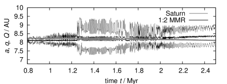
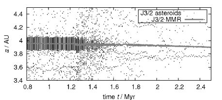
Figure 24: An $N$-body simulation of planetary migration driven by dynamically cold planetesimal disk beyond Neptune, with $10^{3}$ particles and total mass $50\,M_{\oplus}$, and including also $10^{3}$ mass-less particles in the J3/2 resonance with Jupiter. Top: The semimajor axis $a_{\rm S}$ of Saturn vs time and the position of the 1:2 mean motion resonance with Jupiter (estimated from the Kepler law $(1/2)^{-2/3}a_{\rm J}$). Bottom: The same for asteroids initially located inside the J3/2 resonance with Jupiter. The J3/2 asteroids are strongly destabilised at the very time of the 1:2 Jupiter–Saturn resonance crossing ($t=1.25\,{\rm Myr}$) and none of the 1000 test particles survived in the J3/2 region after a mere 0.5 Myr. This means more than $99.9\,\%$ depletion of the primordial population. None of the planetesimal-disk particles got trapped in the J3/2 during or after Jupiter’s and Saturn’s passage through the 1:2 resonance, indicating that more particles are needed to study this process. We used the Mercury hybrid-scheme integrator (Chambers 1999) for the purpose of this test. The gravitational interactions between planets and massive planetesimals are accounted for, but planetesimals do not interact with each other, nor with mass-less test particles. The time step was 36 days and the accuracy parameter $10^{-10}$. Initial conditions of planets were: $a_{\rm J}=5.2$ AU, $a_{\rm S}=8.05$ AU, $a_{\rm U}=12.3$ AU, $a_{\rm N}=17.5$ AU, with all eccentricities and inclination of the order $10^{-3}$. We took the current orbits of Hildas as the initial conditions for our test particles. Note the destabilisation of the Hilda region is neither sensitive to precise initial conditions nor to the mass of the planetesimal disk; the only relevant condition is that Jupiter and Saturn cross their mutual 1:2 resonance.

4.2 The Yarkovsky effect

In Section 3.4 we already discussed the influence of the Yarkovsky effect on the families located inside the J3/2 resonance. In course of time it modified eccentricities of their members, but did not cause a large-scale instability; the families remained inside the resonance all the time. Here we seek the size threshold for which the Yarkovsky would case overall instability by quickly removing the bodies from the resonance.

We perform the following numerical test: we multiply sizes of the long-lived J2/1 objects by fudge factors 0.2, 0.02 and 0.002, for which the Yarkovsky effect is stronger, and compare respective dynamical lifetimes with the original long-lived objects. Results are summarized in Fig. 25. We can conclude that a significant destabilisation of the J2/1 resonant population occurs for sizes ${\sim}\,0.1$ km and smaller (provided the nominal population has sizes mostly 4–12 km).

We do not include the YORP effect (i.e., the torque induced by the infrared thermal emission) at this stage. The YORP is nevertheless theoretically capable to significantly decelerate (or accelerate) the rotation rate, especially of the smallest asteroids, which can lead to random reorientations of the spin axes due to collisions, because the angular momentum is low in this spin-down state. These reorientations can be simulated by a Monte-Carlo model with a typical time scale (Čapek & Vokrouhlický 2004; $R$ is radius in kilometres and $a$ orbital semimajor axis in AU):

$$\tau_{\rm YORP}\simeq 25\,{\rm Myr}\,(R/1\,{\rm km})^{2}\,(2.5\,{\rm AU}/a)^{2}\;.$$ (12)

Since the Yarkovsky effect depends on the obliquity value, the systematic drift would be changed to a random walk for bodies whose spin axis undergo frequent re-orientations by the YORP effect. We can thus expect that the YORP effect might significantly prolong dynamical lifetimes of resonant objects with sizes ${\sim}\,0.1$ km or smaller, because $\tau_{\rm YORP}<0.25\,{\rm Myr}$ for them.

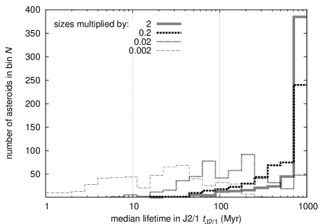
Figure 25: Logarithmic histograms of dynamical lifetimes for the originally long-lived asteroids in the J2/1 resonance, in case the Yarkovsky effect perturbs the orbits. The sizes of the objects (4–12 km) were multiplied by 2, 0.2, 0.02 and 0.002 for comparison. Note a stronger instability starts to occur for the factor 0.02 (i.e., for the sizes 0.08–0.24 km). The YORP reorientations are not included in this model.

We can also check, which orientation of the spin axis makes the escape from the J2/1 resonance more likely to happen. We consider 0.08–0.24 km bodies, clone them 5 times and assign them different values of the obliquity $\gamma=0^{\circ}$, $45^{\circ}$, $90^{\circ}$, $135^{\circ}$ and $180^{\circ}$. Figure 26 shows clearly that the retrograde rotation increases the probability of the escape. This is consistent with the structure of the J2/1 resonance, for which low-$a$ separatrix does not continue to $e=0$. We conclude the remaining very small (yet unobservable) asteroids inside the J2/1 may exhibit a preferential prograde rotation.

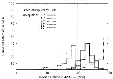
Figure 26: The same as Fig. 25, but now the Yarkovsky effect is calculated only for small bodies (0.08–0.24 km) and varies due to different values of the obliquity $\gamma=0$, $45^{\circ}$, $90^{\circ}$, $135^{\circ}$ and $180^{\circ}$. Note the retrograde bodies (i.e., with a negative drift $da/dt<0$) are significantly more unstable.

We perform a similar simulation for the J3/2 population (first 100 bodies with sizes 10–60 km), but now with YORP reorientations (Eq. 12) included. The results (Fig. 27) show the J3/2 population is much less affected than the J2/1 by the Yarkovsky/YORP perturbation.

We conclude the Yarkovsky/YORP effect may destabilize the J2/1 and J3/2 bodies only partially on the 100 Myr time scale and only for sizes smaller than ${\sim}\,0.1$ km. It is obviously a remote goal to verify this conclusion by observations (note the smallest bodies in these resonances have several kilometers size). Nevertheless, the dynamical lifetimes of small asteroids determined in this section, might be useful for collisional models of asteroid populations, which include also dynamical removal.

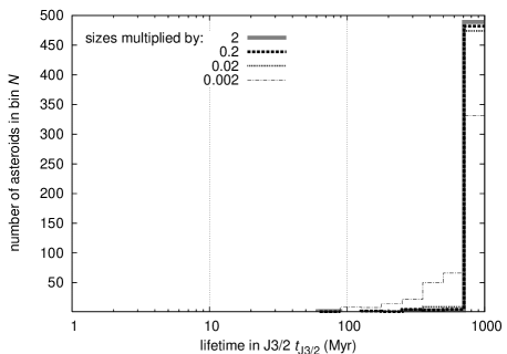
Figure 27: The same as Fig. 25, but for the J3/2 resonance. Instability occurs for the sizes multiplied by 0.002 (i.e., 0.02–0.12 km). The YORP effect and corresponding reorientations of the spin axes are included in this case.

5 Conclusions and future work

The main results of this paper can be summarised as follows: (i) we provided an update of the observed J2/1, J3/2 and J4/3 resonant populations; (ii) we discovered two new objects in the J4/3 resonance; (iii) we described two asteroid families located inside the J3/2 resonance (Schubart and Hilda) and provided an evidence that they are of a collisional origin; (iv) we reported a new mechanism how the Yarkovsky effect systematically changes eccentricities of resonant asteroids; we used this phenomenon to estimate the ages of the Schubart and Hilda families ($(1.7\pm 0.7)$ Gyr and $\gtrsim 4$ Gyr respectively); (v) collisionally-born asteroid clusters in the stable region of J2/1 would disperse in about 1 Gyr; (vi) 20 % of Hildas may escape from the J3/2 resonance within 4 Gyr in the current configuration of planets; (vii) Hildas are strongly unstable when Jupiter and Saturn cross their mutual 1:2 mean motion resonance.

The J3/2 resonance is a unique ‘laboratory’ — the chaotic diffusion is so weak, that families almost do not disperse in eccentricity and inclination due to this effect over the age of the Solar system. What is even more important, they almost do not disperse in semimajor axis, even thought the Yarkovsky effect operates. The drift in $a$ is transformed to a drift in $e$, due to a strong gravitational coupling with Jupiter. We emphasize, this is is not a chaotic diffusion in $e$, but a systematic drift in $e$.

Another piece of information about the families in J3/2 resonance is hidden in the eccentricity $e_{p}$ vs absolute magnitude $H$ plots (see Fig. 28 for the Hilda family). The triangular shape (larger eccentricity dispersion of the family members for larger $H$) is a well-known combination of two effects: (i) larger ejection speed, and (ii) faster dispersal by the Yarkovky forces for smaller fragments. Interestingly, there is also a noticeable depletion of small bodies in the centre of the family and their concentration at the outskirts — a phenomenon known from $(a,H)$ plots of main-belt families, which was interpreted as an interplay between the Yarkovsky and YORP effects (Vokrouhlický et al. 2006). Indeed the estimated $\sim 4$ Gyr age for this family matches the time scale of a YORP cycle for $D\simeq 10$ km asteroids in the Hilda region (e.g., Vokrouhlický & Čapek 2002; Čapek & Vokrouhlický 2004). Vokrouhlický et al. (2006a) pointed out that this circumstance makes the uneven distribution of family members most pronounced.

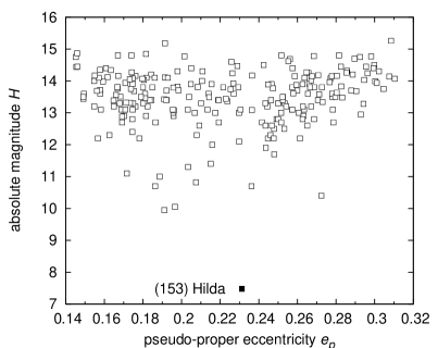
Figure 28: Pseudo-proper eccentricity $e_{p}$ vs absolute magnitude $H$ plot for the members of the Hilda family. The triangular shape and the depletion of asteroids in the centre of the family (around $e_{p}\simeq 0.22$) is discussed in the text.

We postpone the following topics for the future work: (i) a more precise age determination for the resonant asteroid families, based on the Yarkovsky/YORP evolution in the $(e,H)$ space; (ii) a more detailed modelling of analytic or $N$-body migration of planets and its influence on the stability of resonant populations.

Appendix A Resonant Yarkovsky effect

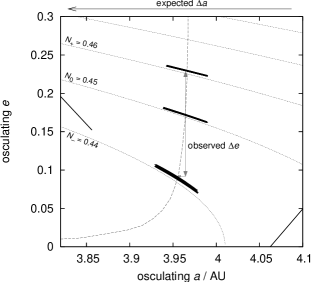
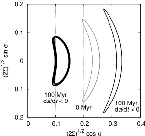
Figure 29: Orbital evolution of two $D=0.1$ km asteroids in the J3/2 resonance within a circular restricted three-body problem (Jupiter on a circular orbit). Obliquities $0^{\circ}$ and $180^{\circ}$ were assigned to the two bodies, such that outside the resonance they would migrate by the Yarkovsky forces in opposite direction. The expected change $\Delta a$ of the semimajor axis in $100$ My is depicted by the arrow on top of the left panel. The left and middle panels show $1$ kyr orbital segments at the beginning and at the end of the simulation: (i) in the semimajor axis $a$ vs eccentricity $e$ projection (left), and (ii) in the projection of Cartesian resonant variables $\sqrt{2\Sigma}\,(\cos\sigma,\sin\sigma)$ (see Eqs. 1 and 2; short-period variations have been removed for better visibility) (middle). The orbits slowly evolve from the initial $N_{0}\simeq 0.45$ level-curve of the integral given by Eq. (5) to their final values of $\simeq 0.44$ ($N_{+}$ with $da/dt>0$) and $\simeq 0.46$ ($N_{-}$ with $da/dt<0$), respectively (see also the right panel). During this evolution the libration centre follows the position of the exact periodic orbit in the J3/2 (dashed curve in the left panel). Because the latter has a steep progression in $e$ as $a$ changes, orbital evolution is characterised by a significant change of the eccentricity $\Delta e$ (also $e_{p}$) but only a small change in $a$ (also $a_{p}$).

The effects of weak dissipative forces, such as the tidal force, gas-drag force and the Poynting-Robertson force, on both non-resonant and resonant orbits were extensively studied in the past (e.g., Murray & Dermott 1999 and references therein). Interaction of the Yarkovsky drifting orbits with high-order, weak resonances was also numerically studied to some extent (e.g., Vokrouhlický & Brož 2002) but no systematic effort was paid to study Yarkovsky evolving orbits in strong low-order resonances. Here we do not intend to develop a detailed theory, rather give a numerical example that can both help to explain results presented in the main text and motivate a more thorough analytical theory.

The Yarkovsky effect outside the resonance. We constructed the following simple numerical experiment: we took the current orbit of (1911) Schubart as a starting condition and integrated the motion of two 0.1 km size objects with extreme obliquity values $0^{\circ}$ and $180^{\circ}$. Their thermal parameters were the same as in Section 3.4. Because the diurnal variant of the Yarkovsky effect dominates the evolution, the extreme obliquities would mean the two test bodies would normally (outside any resonances) drift in semimajor axis in two opposite directions (e.g., Bottke et al. 2002, 2006). The two orbits would secularly acquire $\Delta a\simeq+0.25$ AU or $-0.25$ AU in 100 My, about the extent shown by the arrow on top of the left panel of Fig. 29. Since the strength of the Yarkovsky forces is inversely proportional to the size, we can readily scale the results for larger bodies.

The resonance without the Yarkovsky effect. If we include gravitational perturbations by Jupiter only, within a restricted circular three body problem ($e_{\rm J}=0$), and remove short-period oscillations by a digital filter, the parameter $N$ from Eq. (5) would stay constant. The orbit would be characterized by a stable libration in $(\Sigma,\sigma)$ variables with about $30^{\circ}$ amplitude in $\sigma$ (see the curve labelled 0 Myr in the middle panel of Fig. 29).

While evolving, some parameters known as the adiabatic invariants are approximately conserved (see, e.g., Landau & Lifschitz 1976; Henrard 1982; Murray & Dermott 1999). One of the adiabatic invariants is $N$ itself. Another, slightly more involved quantity, is the area $J$ enclosed by the resonant path in the $\sqrt{2\Sigma}\,(\cos\sigma,\sin\sigma)$ space:

$$J=\oint\sqrt{2\Sigma}\,d\sigma\;.$$ (13)

We would thus expect these parameters be constant, except for strong-enough perturbation or long-enough time scales (recall the adiabatic invariants are constant to the second order of the perturbing parameter only).

Resonant Yarkovsky effect. Introducing the Yarkovsky forces makes the system to evolve slowly. The lock in the resonance prevents the orbits to steadily drift away in the semimajor axis and the perturbation by the Yarkovsky forces acts adiabatically. This is because (i) the time scale of the resonance oscillations is much shorter than the characteristic time scale of the orbital evolution driven by the Yarkovsky forces, and (ii) the strength of the resonant terms in the equations of motion are superior to the strength of the Yarkovsky accelerations.

We let the two J3/2 orbits evolve over 100 Myr (Fig. 29). At the end of our simulation the orbits moved from $N_{0}\simeq 0.45$ to $N_{+}\simeq 0.46$ (for the outward migrating orbit) or to $N_{-}\simeq 0.44$ (for the inward migrating orbit), respectively. During this evolution, both orbits remained permanently locked in the J2/1 resonance, librating about the periodic orbit (dashed line in the left panel of Fig. 29). Because the position of this centre has a steep progression in the eccentricity and only small progression in the semimajor axis, the evolution across different $N$-planes makes the orbital eccentricity evolve significantly more than the semimajor axis. This is also seen in the middle panel of Fig. 29, where the librating orbits significantly split farther/closer with respect to origin of coordinates (note the polar distance from the origin is basically a measure of the eccentricity). The shape of the librating orbit is modified such that the area $J$ stays approximately constant. We have verified that the relative change in both adiabatic invariants, acquired during the 100 Myr of evolution, is about the same: $\delta N/N\sim\delta J/J\sim 5\times 10^{-2}$. It is a direct expression of the strength of the perturbation by the Yarkovsky forces.

We can conclude the Yarkovsky effect results in a significantly different type of secular evolution for orbits initially inside strong first-order mean motion resonances with Jupiter. Instead of secularly pushing the orbital semimajor axis inward or outward from the Sun, it drives the orbital eccentricity to smaller or larger values, while leaving the semimajor axis to follow the resonance centre.

If we were to leave the orbital evolution continue in our simple model, the inward-migrating orbit would leave the resonance toward the zone of low-eccentricity apocentric librators. Such bodies are observed just below the J2/1 resonance. On the other hand, the outward-migrating orbit would finally increase the eccentricity to the value when the orbit starts to cross the Jupiters orbit. Obviously, in a more complete model, with all planets included, the orbits would first encounter the unstable region surrounding the stable resonant zone. Such marginally stable populations exist in both the J3/2 and J2/1 resonances.

References

- [] Beaugé C., Roig F., 2001, Icarus, 153, 391
- [] Bottke W. F., Vokrouhlický D., Brož M., Nesvorný D., Morbidelli A., 2001, Sci, 294, 1693
- [] Bottke W. F., Vokrouhlický D., Rubincam D. P., Brož M., 2002, in Bottke W.F., Cellino A., Paolicchi P., Binzel R.P., eds., Asteroids III. University of Arizona Press, Tucson, p. 395
- [] Bottke W. F., Durda D. D., Nesvorný D., Jedicke R., Morbidelli A., Vokrouhlický D., Levison H. F., 2005, Icarus, 179, 63
- [] Bottke W. F., Vokrouhlický D., Rubincam D. P., Nesvorný D., 2006, Annu. Rev. Earth Planet. Sci., 34, 157
- [] Brown M.E., Barkume K.M., Ragozzine D., Schaller E.L., 2007, Nature, 446, 294
- [] Brož M., Vokrouhlický D., Roig F., Nesvorný D., Bottke W.F., Morbidelli A., 2005, MNRAS, 359, 1437
- [] Brož M., 2006, PhD thesis, Charles University (see at http://sirrah.troja.mff.cuni.cz/~mira/mp/)
- [] Bus S.J., Vilas F., Barucci M.A., 2002, in Bottke W.F., Cellino A., Paolicchi P., Binzel R.P., eds., Asteroids III. University of Arizona Press, Tucson, p. 169
- [] Čapek D., Vokrouhlický D., 2004, Icarus, 172, 526
- [] Chambers J.E., 1999, MNRAS, 304, 793
- [] Dahlgren M., 1998, A&A, 336, 1056
- [] Dahlgren M., Lagerkvist C.-I., 1995, A&A, 302, 907
- [] Dahlgren M., Lagerkvist C.-I., Fitzsimmons A., Williams I. P., Gordon M., 1997, A&A, 323, 606
- [] Dahlgren M., Lahulla J.F., Lagerkvist C.-I., Lagerros J., Mottola S., Erikson A., Gonano-Beurer M., di Martino M., 1998, Icarus, 133, 247
- [] Dahlgren M., Lahulla J.F., Lagerkvist C.-I., 1999, Icarus, 138, 259
- [] Davis D.R., Durda D.D., Marzari F., Campo Bagatin A., Gil-Hutton R., 2002, in Bottke W.F., Cellino A., Paolicchi P., Binzel R.P., eds., Asteroids III. University of Arizona Press, Tucson, p. 545
- [] Dell’Oro A., Marzari F., Paolicchi P., Vanzani A., 2001, A&A, 366, 1053
- [] Dohnanyi J.W., 1969, J. Geophys. Res., 74, 2531
- [] Durda D., Bottke W.F., Nesvorny D., Encke B., Merline W.J., Asphaug E., Richardson D.C., 2007, Icarus, 186, 498
- [] Farinella P., Gonczi R., Froeschlé Ch., Froeschlé C., 1993, Icarus, 101, 174
- [] Farinella P., Froeschlé C., Gonczi R., 1994, in Milani A., Di Martino M., Cellino A., eds., Asteroids, comets, meteors 1993. Kluwer Academic Publishers, Dordrecht, p. 205
- [] Ferraz-Mello S., 1988, AJ, 96, 400
- [] Ferraz-Mello S., Michtchenko T.A., 1996, A&A, 310, 1021
- [] Ferraz-Mello S., Michtchenko T.A., Nesvorný D., Roig F., Simula, A., 1998a, Planet. Sp. Sci., 46, 1425
- [] Ferraz-Mello S., Michtchenko T.A., Roig F., 1998b, AJ, 116, 1491
- [] Gil-Hutton R., Brunini A., 2008, Icarus, 193, 567
- [] Gomes R., Levison H. L., Tsiganis K., Morbidelli A., 2005, Nature, 435, 466
- [] Hahn J. M., Malhotra R., 1999, AJ, 117, 3041
- [] Henrard J., 1982, Celest. Mech., 27, 3
- [] Ivezić Z., Jurić M., Lupton R.H., Tabachnik S., Quinn T., 2002, Survey and other telescope technologies and discoveries, (J.A. Tyson, S. Wolff, Eds.) Proceedings of SPIE Vol. 4836
- [] Jedicke R., Magnier E.A., Kaiser N., Chambers K.C., 2007, in Milani A., Valsecchi G.B., Vokrouhlický D., eds., Near Earth Asteroids, our Celestial Neighbors. Cambridge University Press, Cambridge, p. 341
- [] Kenyon S. J., Bromley B. C., O’Brien D. P., Davis D. R., 2008, in Barucci M.A., Boehnhardt H., Cruikshank D.P., Morbidelli A., eds., The Solar System beyond Neptune. University of Arizona Press, Tucson, p. 293
- [] Krueger A., 1889, AN, 120, 221
- [] Kühnert F., 1876, AN, 87, 173
- [] Landau L. D., Lifschiz E. M., 1976, Mechanics, Pergamon Press, Oxford
- [] Laskar J., Robutel P., 2001, Celest. Mech. Dyn. Astron., 80, 39
- [] Lemaitre A., Henrard J., 1990, Icarus, 83, 391
- [] Levison H., Duncan M., 1994, Icarus, 108, 18
- [] Malhotra R., 1995, AJ, 110, 420
- [] Michtchenko T. A., Ferraz-Mello S., 1997, Planet. Sp. Sci., 45, 1587
- [] Milani A., 1993, Celest. Mech. Dyn. Astron., 57, 59
- [] Milani A., Farinella P., 1995, Icarus, 115, 209
- [] Morbidelli A., Moons M., 1993, Icarus, 102, 316
- [] Morbidelli A., Levison H. L., Tsiganis K., Gomes R., 2005, Nature, 435, 462
- [] Morbidelli A., Tsiganis K., Crida A., Levison H.F., Gomes R., 2007, AJ, 134, 1790
- [] Moons M., Morbidelli A., Migliorini F., 1998, Icarus, 135, 458
- [] Murray C. D., 1986, Icarus, 65, 70
- [] Murray C. D., Dermott S. F., 1999, Solar System Dynamics, Cambridge University Press, Cambridge
- [] Nesvorný D., Ferraz-Mello S., 1997, Icarus, 130, 247
- [] Nesvorný D., Beaugé C., Dones L., 2004, AJ, 127, 1768
- [] Nesvorný D., Vokrouhlický D., Bottke W.F., 2006, Science, 312, 1490
- [] Nesvorný D., Bottke W.F., Dones L., Levison H.F., 2002, Nature, 417, 720
- [] Nesvorný D., Alvarellos J.L.A., Dones L., Levison H.F., 2003, AJ, 126, 398
- [] Nesvorný D., Jedicke R., Whiteley R.J., Ivezić Z., 2005, Icarus, 173, 132
- [] O’Brien D.P., Greenberg R., 2003, Icarus, 164, 334
- [] Palisa J., 1888, AN, 120, 111
- [] Press W. R., Teukolsky S. A., Vetterling W., Flannery B. P., 2007, Numerical Recipes: The Art of Scientific Computing, Cambridge University Press, Cambridge
- [] Quinn T.R., Tremaine, S., Duncan, M. 1991, AJ, 101, 2287
- [] Roig F., Gil-Hutton R., 2006, Icarus, 183, 411
- [] Roig F., Nesvorný D., Ferraz-Mello S., 2002, MNRAS, 335, 417
- [] Roig F., Ribeiro A. O., Gil-Hutton R., 2008, A&A, in press
- [] Schubart J., 1982a, A&A, 114, 200
- [] Schubart J., 1982b, Cel. Mech. Dyn. Astron., 28, 189
- [] Schubart J., 1991, A&A, 241, 297
- [] Schubart J., 2007, Icarus, 188, 189
- [] Sessin W., Bressane B.R., 1988, Icarus, 75, 97
- [] Tanga P., Cellino A., Michel P., Zappalà V., Paolicchi P., Dell’Oro A., 1998, Icarus, 141, 65
- [] Tedesco E.F., Noah P.V., Noah M., Price S.D., 2002, AJ, 123, 1056
- [] Tsiganis K., Knežević Z., Varvoglis H., 2007, Icarus, 186, 484
- [] Tsiganis K., Gomes R., Morbidelli A., Levison H.L., 2005, Nature, 435, 459
- [] Tsuchida M., 1990, Rev. Mexicana Astron. Astrophys., 21, 585
- [] Vokrouhlický D., Brož, 2002, in Celletti A., Ferraz-Mello S., Henrard J., eds., Modern Celestial Mechanics: from Theory to Applications. Kluwer Academic Publishers, Dordrecht, p. 467
- [] Vokrouhlický D., Brož M., Bottke W.F., Nesvorný D., Morbidelli A., 2006a, Icarus, 182, 118
- [] Vokrouhlický D., Brož M., Morbidelli A., Bottke W.F., Nesvorný D., Lazzaro D., Rivkin A. S., 2006b, Icarus, 182, 92
- [] Weissman P.R., Bottke W.F., Levison H.L., 2002, in Bottke W.F., Cellino A., Paolicchi P., Binzel R.P., eds., Asteroids III. University of Arizona Press, Tucson, p. 669
- [] Zappalà V., Cellino A., Farinella P., Knežević Z., 1990, AJ, 100, 2030
- [] Zappalà V., Cellino A., Farinella P., Milani A., 1994, AJ, 107, 772
- [] Zappalà V., Cellino A., Dell’Oro A., Paolicchi P., 2002, in Bottke W.F., Cellino A., Paolicchi P., Binzel R.P., eds., Asteroids III. University of Arizona Press, Tucson, p. 619