S

Abstract

The uncoupled Continuous Time Random Walk ($CTRW$) in one space-dimension and under power law regime is splitted into three distinct random walks: ($rw_{1}$), a random walk along the line of natural time, happening in operational time; ($rw_{2}$), a random walk along the line of space, happening in operational time; ($rw_{3}$), the inversion of ($rw_{1}$), namely a random walk along the line of operational time, happening in natural time. Via the general integral equation of $CTRW$ and appropriate rescaling, the transition to the diffusion limit is carried out for each of these three random walks. Combining the limits of ($rw_{1}$) and ($rw_{2}$) we get the method of parametric subordination for generating particle paths, whereas combination of ($rw_{2}$) and ($rw_{3}$) yields the subordination integral for the sojourn probability density in space - time fractional diffusion.

FRACALMO PRE-PRINT:  http://www.fracalmo.org

The European Physical Journal, Special Topics, Vol. 193 (2011) 119–132

Special issue: Perspectives on Fractional Dynamics and Control

Guest Editors: Changpin LI and Francesco MAINARDI

 

ubordination Pathways to Fractional Diffusion

Rudolf GORENFLO ⁽¹⁾ and Francesco MAINARDI^{(2) (1)} Department of Mathematics and Informatics, Free University Berlin,

Arnimallee 3, D-14195 Berlin, Germany

E-mail: gorenflo@mi.fu-berlin.de

⁽²⁾ Department of Physics, University of Bologna, and INFN,

Via Irnerio 46, I-40126 Bologna, Italy

Corresponding Author. E-mail: francesco.mainardi@unibo.it

2000 Mathematics Subject Classification: 26A33, 33E12, 33C60, 44A10, 45K05, 60G18, 60G50, 60G52, 60K05, 76R50.

Key Words and Phrases: Fractional derivatives, Fractional integrals, Fractional diffusion, Mittag-Leffler function, Wright function, Continuous Time Random Walk, Power laws, Subordination, Renewal processes, Self-similar stochastic processes.

1. Introduction

In recent decades the notion of continuous time random walk has become popular as a conceptual and computational model for diffusion processes. Its relation to continuous diffusion processes is an asymptotic one, either by considering spatial and temporal refinement or by looking for large-time wide-space behaviour (both views being equivalent to change the units of measurement in time and space). Often such walks are considered for power law behaviour of waiting times and jumps, and from the behaviour in the Laplace-Fourier domain near zero the relevant limiting diffusion equations are deduced heuristically. There are several methods of making precise this transition to the limit, the fundamental role being played by the domains of attraction of stable probability laws (in time and space). It is desirable to have presentations of this transition without much theory of abstract probability and stochastic processes, and this can be done in a transparent manner for the derivation of the limiting fractional diffusion equations. The essential idea of our approach presented here is to use the integral equation of continuous time random walk separately for three random walks obtained by splitting the original walk, and then synthesizing the results. We so obtain our method of ”parametric subordination” as well as what usually is called ”subordination” in fractional diffusion.

2. The Space-Time Fractional Diffusion

We begin by considering the Cauchy problem for the (spatially one-dimensional) space-time fractional diffusion (STFD) equation.

$${\,{}_{t}}D_{*}^{\,\beta}\,u(x,t)\,=\,{\,{}_{x}}D_{\theta}^{\,\alpha}\,u(x,t)\,,\quad u(x,0)=\delta(x)\,,\quad x\in\vbox{\hbox to8.9pt{I\hskip-2.1ptR\hfil}}\;,\quad t\geq 0\,,$$

where {$\alpha\,,\,\theta\,,\,\beta$} are real parameters restricted to the ranges

$$0<\alpha\leq 2\,,\quad|\theta|\leq\min\{\alpha,2-\alpha\}\,,\quad 0<\beta\leq 1\,.$$

Here ${\,{}_{t}}D_{*}^{\,\beta}$ denotes the Caputo fractional derivative of order $\beta$, acting on the time variable $t$, and ${\,{}_{x}}D_{\,\theta}^{\,\alpha}$ denotes the Riesz-Feller fractional derivative of order $\alpha$ and skewness $\theta$, acting on the space variable $x$. Let us note that the solution $u(x,t)$ of the Cauchy problem (2.1), known as the Green function or fundamental solution of the space-time fractional diffusion equation, is a probability density in the spatial variable $x$, evolving in time $t$. In the case $\alpha=2$ and $\beta=1$ we recover the standard diffusion equation for which the fundamental solution is the Gaussian density with variance $\sigma^{2}=2t$.

Writing, with $\hbox{Re}[s]>\sigma_{0}$, $\kappa\in\vbox{\hbox to8.9pt{I\hskip-2.1ptR\hfil}}\;$, the transforms of Laplace and Fourier as

$${{\cal L}}\left\{f(t);s\right\}=\widetilde{f}(s):=\int_{0}^{\infty}{\rm e}^{\displaystyle\,-st}\,f(t)\,dt\,,$$

$${{\cal F}}\left\{g(x);\kappa\right\}=\widehat{g}(\kappa):=\int_{-\infty}^{+\infty}\!\!{\rm e}^{\,\displaystyle i\kappa x}\,g(x)\,dx\,,$$

we have the corresponding transforms of ${\,{}_{t}}D_{*}^{\,\beta}f(t)$ and ${\,{}_{x}}D_{\,\theta}^{\,\alpha}g(x)$ as

$${{\cal L}}\left\{{\,{}_{t}}D_{*}^{\,\beta}\,f(t)\right\}=s^{\,\displaystyle\beta}\,\widetilde{f}(s)-s^{\,\displaystyle\beta-1}\,f(0)\,,$$

$${{\cal F}}\left\{{\,{}_{x}}D_{\,\theta}^{\,\alpha}\,g(x)\right\}=-|\kappa|^{\,\displaystyle\alpha}\,i^{\,\displaystyle\theta\,\hbox{sign}\,\kappa}\,\widehat{g}(\kappa)\,.$$

Notice that $i^{\,\displaystyle\theta\,\hbox{sign}\,\kappa}={\rm exp}\,[i\,(\hbox{sign}\,\kappa)\,\theta\,\pi/2]$. For the mathematical details the interested reader is referred to Gorenflo and Mainardi (1997), Podlubny (1999), Butzer and Westphal (2000), Kilbas, Srivastava and Trujillo (2006), Hilfer (2008), Tomovski, Hilfer and Srivastava (2010) on fractional derivatives, and to Samko, Kilbas and Marichev (1993), Rubin (1996), on the Feller potentials.

For our purposes let us here confine ourselves to recall the representation in the Laplace-Fourier domain of the (fundamental) solution of (2.1) as it results from the application of the transforms of Laplace and Fourier. Using $\widehat{\delta}(\kappa)\equiv 1$ we have from (2.1)

$$s^{\,\displaystyle\beta}\,\widehat{\widetilde{u}}(\kappa,s)-s^{\,\displaystyle\beta-1}=-|\kappa|^{\,\displaystyle\alpha}\,i^{\,\displaystyle\theta\,\hbox{sign}\,\kappa}\,\widehat{\widetilde{u}}(\kappa,s)\,,$$

hence

$$\widehat{\widetilde{u}}(\kappa,s)=\frac{s^{\,\displaystyle\beta-1}}{s^{\,\displaystyle\beta}+|\kappa|^{\,\displaystyle\alpha}\,i^{\,\displaystyle\theta\,\hbox{sign}\,\kappa}}\,.$$

For explicit expressions and plots of the fundamental solution of (2.1) in the space-time domain we refer the reader to Mainardi, Luchko and Pagnini (2001). There, starting from the fact that the Fourier transform $\widehat{u}(\kappa,t)$ can be written as a Mittag-Leffler function with complex argument, the authors have derived a Mellin-Barnes integral representation of $u(x,t)$ with which they have proved the non-negativity of the solution for values of the parameters $\{\alpha,\,\theta,\,\beta\}$ in the range (2.2) and analyzed the evolution in time of its moments. In particular for $\{0<\alpha<2,\,\beta=1\}$ we obtain the stable densities of order $\alpha$ and skewness $\theta$. The representation of $u(x,t)$ in terms of Fox $H$-functions can be found in Mainardi, Pagnini and Saxena (2005), see also Chapter 6 in the book by Mathai, Saxena and Haubold (2010). We note, however, that the solution of the STFD Equation (2.1) and its variants has been investigated by several authors; let us only mention some of them, Barkai (2001), Meerschaert et al. (2002 and 2004), Metzler and Klafter (2004), where the connection with the $CTRW$ was also pointed out.

3. The Continuous-Time Random Walk

Starting in the Sixties and Seventies of the past century the concept of continuous time random walk, $CTRW$, became popular in physics as a rather general (microscopic) model for diffusion processes, see the monograph by Weiss (1994). Mathematically, a $CTRW$ is a renewal process with rewards or a random-walk subordinated to a renewal process, and has been treated as such by Cox (1967). It is generated by a sequence of independent identically distributed ($iid$) positive waiting times $T_{1},T_{2},T_{3},\dots$, each having the same probability distribution $\Phi(t)$, $t\geq 0$, of waiting times $T$, and a sequence of $iid$ random jumps $X_{1},X_{2},X_{3},\dots$, each having the same probability distribution function $W(x)$, $x\in\vbox{\hbox to8.9pt{I\hskip-2.1ptR\hfil}}\;$, of jumps $X$. These distributions are assumed to be independent of each other. Allowing generalized functions (interpretable as measures), we have corresponding probability densities $\phi(t)=\Phi^{\prime}(t)$ and $w(x)=W^{\prime}(x)$ that we will use for ease of notation. Setting $t_{0}=0$, $t_{n}=T_{1}+T_{2}+\dots+T_{n}$ for $n\in{\rm I\hskip-2.0ptN}$, and $x_{0}=0$, $x_{n}=X_{1}+X_{2}+\dots+X_{n}$, $x(t)=x_{n}$ for $t_{n}\leq t<t_{n+1}$, we get a (microscopic) model of a diffusion process. A wandering particle starts in $x_{0}=0$ and makes a jump $X_{n}$ at each instant $t_{n}$. Natural probabilistic reasoning then leads us to the integral equation of continuous time random walk for the probability density $p(x,t)$ of the particle being in position $x$ at instant $t\geq 0$:

$$p(x,t)=\delta(x)\,\Psi(t)\,+\int_{0}^{t}\!\!\phi(t-t^{\prime})\,\left[\int_{-\infty}^{+\infty}\!\!w(x-x^{\prime})\,p(x^{\prime},t^{\prime})\,dx^{\prime}\right]\,dt^{\prime}\,,$$

Here the survival probability

$$\Psi(t)=\int_{t}^{\infty}\phi(t^{\prime})\,dt^{\prime}$$

denotes the probability that at instant $t$ the particle still is sitting in its initial position $x_{0}=0$. Eq. (3.1) is also known as (semi –) Markov renewal equation. Germano et al. (2009), considering the more general situation of coupled CTRW, have given a detailed stochastic proof of an integral equation which by modification and specialization reduces to (3.1).

By using the Fourier and Laplace transforms we arrive, via $\widehat{\delta}(\kappa)\equiv 1$ and the convolution theorems, in the transform domain at the equation

$$\widehat{\widetilde{p}}(\kappa,s)=\widetilde{\Psi}(s)+\widehat{w}(\kappa)\,\widetilde{\phi}(s)\,\widehat{\widetilde{p}}(\kappa,s)\,,$$

which, by $\widetilde{\Psi}(s)=(1-\widetilde{\phi}(s))/s$ implies the Montroll-Weiss equation, see e.g Weiss (1994),

$$\widehat{\widetilde{p}}(\kappa,s)=\frac{1-\widetilde{\phi}(s))}{s}\,\frac{1}{1-\widehat{w}(\kappa)\,\widetilde{\phi}(s)}\,.$$

Because of $|\widehat{w}(\kappa)|<1$, $|\widetilde{\phi}(s)|<1$ for $\kappa\neq 0$, $s\neq 0$, we can expand

$$\widehat{\widetilde{p}}(\kappa,s)=\widetilde{\Psi}(s)\,\sum_{n=0}^{\infty}\,\left[\widetilde{\phi}(s)\,\widehat{w}(\kappa)\right]^{n}\,,$$

and promptly obtain, see e.g. Cox (1967) and Weiss (1994),

$$p(x,t)=\sum_{n=0}^{\infty}v_{n}(t)\,w_{n}(x)\,\quad-\infty<x<+\infty,t\geq 0\,.$$

Here the functions $v_{n}=\Psi\,*\,\phi^{*n}$ and $w_{n}=w^{*n}$ are obtained by iterated convolutions in time $t$ and in space $x$, respectively; in particular we have:

$$v_{0}(t)=(\Psi\,*\,\delta)(t)=\Psi(t),\;v_{1}(t)=(\Psi\,*\,\phi)(t),\;w_{0}(x)=\delta(x),\;w_{1}(x)=w(x).$$

The representation (3.6) can be found without the detour over (3.4) by direct probabilistic treatment. It exhibits the $CTRW$ as a subordination of a random walk to a renewal process.

Note that in the special case $\phi(t)=m\,{\rm exp}\,(-mt)$, $m>0$, the equation (3.1) describes the compound Poisson process. It reduces after some manipulations to the Kolmogorov-Feller equation

$$\frac{\partial}{\partial t}p(x,t)=-mp(x,t)+m\int_{-\infty}^{+\infty}w(x-x^{\prime})p(x^{\prime},t)\,dx^{\prime}\,.$$

From (3.6) we then obtain the well-known series representation

$$p(x,t)={\rm e}^{-mt}\,\sum_{n=0}^{\infty}\frac{(mt)^{n}}{n!}\,w_{n}(x)\,.$$

4. Power Law Assumptions and Well-Scaled Passage to the Diffusion Limit

We will pass to the diffusion limit of $CTRW$ under power law assumptions for waiting times and jumps given by asymptotic relations

$$1-\widetilde{\phi}(s)\sim\lambda s^{\beta},\quad\lambda>0,\quad s\to 0^{+}\,,$$

$$1-\widehat{w}(\kappa)\sim\mu|\kappa|^{\alpha}\,i^{\displaystyle\,\theta\,\hbox{sign}\,\kappa}\,,\quad\mu>0\,,\quad\kappa\to 0\,,$$

where $\beta$, $\alpha$ and $\theta$ are restricted as in (2.2). See, e.g. Gorenflo and Mainardi (2003), Scalas, Gorenflo and Mainardi (2004), Gorenflo (2010) for their physical meaning, obtainable via Tauber-Karamata theorems on aymptotics. We rescale space and time by multiplying the jumps $X_{k}$ and waiting times $T_{k}$ by positive factors $h$ and $\tau$ (intended to be sent to zero), so obtaining a rescaled walk

$$x_{n}(h)=\sum_{k=1}^{n}h\,X_{k}\,,\quad t_{n}(\tau)=\sum_{k=1}^{n}\tau\,T_{k}\,.$$

Physically, this amounts to changing the units of measurement from $1$ to $1/h$ in space $x$, from $1$ to $1/\tau$ in time $t$.

For the reduced jumps and waiting times we get

$$w_{h}(x)=w(x/h)/h\,,\quad\phi_{\tau}(t)=\phi(t/\tau)/\tau\,,$$

$$\widehat{w}_{h}(\kappa)=\widehat{w}(h\kappa),,\quad\widetilde{\phi}_{\tau}(s)=\widetilde{\phi}(\tau s)\,,$$

and the Montroll-Weiss equation (3.3) transforms into

$$\widehat{\widetilde{p}}_{h,\tau}(\kappa,s)\!=\!\frac{1-\widetilde{\phi}_{\tau}(s)}{s}\,\frac{1}{1-\widehat{w}_{h}(\kappa)\,\widetilde{\phi}_{\tau}(s)}\!=\!\frac{1-\widetilde{\phi}(\tau s)}{s}\,\frac{1}{1-\widehat{w}(h\kappa)\,\widetilde{\phi}(\tau s)}\,.$$

Using our power law assumptions (4.1), (4.2) we find, for $h\to 0$, $\tau\to 0$, the asymptotics

$$\widehat{\widetilde{p}}_{h,\tau}(\kappa,s)\sim{\displaystyle\frac{\lambda\tau^{\beta}s^{\beta-1}}{\mu(h|\kappa|)^{\alpha}\,i^{\displaystyle\theta\,\hbox{sign}\,\kappa}+\lambda(\tau s)^{\beta}}}={\displaystyle\frac{s^{\beta-1}}{\rho(h,\tau)\,|\kappa|^{\alpha}\,i^{\displaystyle\theta\,\hbox{sign}\,\kappa}+s^{\beta}}}$$

with

$$\rho(h,\tau)=\frac{\mu h^{\alpha}}{\lambda\tau^{\beta}}\,.$$

Adopting the scaling relation

$$\rho(h,\tau)=\frac{\mu h^{\alpha}}{\lambda\tau^{\beta}}=1\,,$$

we arrive for $h\to 0$ at the limit

$$\widehat{\widetilde{p}}_{0,0}(\kappa,s)={\displaystyle\frac{s^{\beta-1}}{|\kappa|^{\alpha}\,i^{\displaystyle\theta\,\hbox{sign}\,\kappa}+s^{\beta}}}=:\widehat{\widetilde{u}}(\kappa,s)$$

which we identify as the Fourier-Laplace solution to the Cauchy problem (2.1) for the STFD equation. By inverting the Laplace transform and then for the Fourier transform invoking the continuity theorem of probability theory we get weak convergence to the fundamental solution of (2.1).

Remark. Because Mittag-Leffler waiting times distributed according to $\Psi(t)=E_{\beta}(-t^{\beta})$ play a distinguished role among power law waiting times and lead to time–fractional CTRW, in fact to the time–fractional Kolmogorov–Feller equation, see e.g. Hilfer (1995), Hilfer and Anton (1995), Gorenflo and Mainardi (2008) and Gorenflo (2010), it is natural to use them (properly scaled) for approximately simulating particle paths of space-time fractional diffusion processes. Fulger, Scalas and Germano (2008) have done this, thereby using exact methods for generating the required temporal Mittag-Leffler deviates and spatial stable deviates, giving references for these methods.

5. Splitting into Three Random Walks

We analyze the anatomy of the $CTRW$ of Section 3 by splitting it into three random walks ($rw_{1}$), ($rw_{2}$), ($rw_{3}$) that we will treat in analogy to our method of well-scaled transition to the diffusion limit. We will work in three coordinates: the semiaxis $t\geq 0$ of natural time, the semi-axis $t_{*}\geq 0$ of operational time, the axis $-\infty<x<+\infty$ of space. In addition to the Laplace transform ${\cal L}\{f(t);s\}=\widetilde{f}(s)$ with respect to $t$ we will need the Laplace transform ${\cal L}\{f(t_{*});s_{*}\}=\widetilde{f}(s_{*})$ with respect to $t_{*}$.

For convenience let us denote by ($rw$) $\,\equiv\,$ ($CTRW$) the random walk of Section 3,

$$t_{0}=0\,,\;t_{n}=T_{1}+T_{2}+\dots+T_{n}\,;\quad x_{0}=0\,,\;x_{n}=X_{1}+X_{2}+\dots+X_{n}\,.$$

This is a random walk along the space line $x\in\vbox{\hbox to8.9pt{I\hskip-2.1ptR\hfil}}\;$ happening in physical time $t\geq 0$. Here $\phi(t)$ is the waiting time density, $w(x)$ is the jump density, and $p(x,t)$ is the sojourn density in point $x$ at instant $t$.

By ($rw_{1}$) we denote the basic renewal process

$$t_{*,n}=n\,(n=0,1,2,\dots)\,;\quad t_{0}=0\,,\;t_{n}=T_{1}+T_{2}+\dots+T_{n}\,.$$

We consider it as a random walk along natural time $t\geq 0$, happening in operational time $t_{*}\geq 0$. Here $t_{*}$ plays the role of a “pseudo time”, $t$ plays the role of “pseudo space”. The waiting time (in $t_{*}$) is constant (fixed) =1, so we have the “waiting time” density $v(t_{*})=\delta(t_{*}-1)$. The jump instants are the integers $t_{*n}=n>0$, and we set $t_{*0}=0$. The “jump density” (in $t$) is $\phi(t)$. We denote the “sojourn density” in “point” $t$ at “instant” $t_{*}$ by $r(t,t_{*})$. Note that in this sojourn density $r$ the first argument is the pseudo space $t$, whereas the second argument is pseudo time $t_{*}$.

By ($rw_{2}$) we denote the random walk

$$t_{*,n}=n\,(n=0,1,2,...)\,;\quad x_{0}=0\,,\;x_{n}=X_{1}+X_{2}+\dots+X_{n}\,,$$

which we consider as a random walk along natural space $x\in\vbox{\hbox to8.9pt{I\hskip-2.1ptR\hfil}}\;$, happening in operational time $t_{*}\geq 0$ which (again) plays the role of ”pseudo time”. But $x$ here is the usual spatial variable. The waiting time density in $t_{*}$ is (again) $v(t_{*})=\delta(t_{*}-1)$, the jump density is $w(x)$, and we denote the sojourn density in point $x$ at ”instant” $t_{*}$ by $\xi(x,t_{*})$.

By ($rw_{3}$) we denote the random walk

$$t_{0}=0\,,\;t_{n}=T_{1}+T_{2}+\dots+T_{n}\,;\quad t_{*n}=n\,(n=0,1,2,...)\,,$$

along the semi-axis $t_{*}\geq 0$ happening in physical time $t\geq 0$. The walk is just the inversion of ($rw_{1}$). The variable $t$ now plays the role of time, the waiting time density is $\phi(t)$. But $t_{*}$ plays the role of ”pseudo space”, the jump density being $v(t_{*})=\delta(t_{*}-1)$. The sojourn density in ”point” $t_{*}$ at instant $t$ is denoted by $q(t_{*},t)$ where the pseudo space $t_{*}$ is the first argument and time $t$ is the second argument.

6. Asymptotic Analysis of the Three Walks

In ($rw_{1}$) and ($rw_{3}$) we have walks in the positive pseudo-space direction. For such walks it is convenient to modify the Montroll-Weiss formula by using the Laplace transform in place of the Fourier transform. If in the general ($CTRW$) the jump density $w(x)\geq 0$ for all $x\in\vbox{\hbox to8.9pt{I\hskip-2.1ptR\hfil}}\;$ then with

$$\widetilde{g}(\kappa):=\int_{0}^{\infty}\!\!g(x)\,{\rm e}^{-\kappa x}\,dx\,,\quad\kappa\geq\kappa_{0}\,,$$

we can replace the original Montroll-Weiss equation (3.4) by

$$\widetilde{\widetilde{p}}(\kappa,s)=\frac{1-\widetilde{\phi}(s)}{s}\,\frac{1}{1-\widetilde{w}(\kappa)\,\widetilde{\phi}(s)}\,.$$

Here for ($rw_{1}$) and ($rw_{3}$) the specifically relevant replacements of $x$ and $t$, $\kappa$ and $s$ must be made, analogously for ($rw_{2}$) in (3.3) and (3.4). Analogous to Section 4 we will carry out well-scaled transitions to the diffusion limit, observing (4.1) and (4.2) and an additional asymptotic relation for the Laplace transform of $v(t_{*})=\delta(t_{*}-1)$. We have

$$\widetilde{v}(s_{*})={\rm e}^{-s_{*}}=1-s_{*}+o(s_{*})\,,\quad\hbox{for}\quad s_{*}\to 0\,.$$

6.1 Analysis of ($rw_{1}$).

In place of (6.2) we have

$$\widetilde{\widetilde{r}}(s,s_{*})=\frac{1-\widetilde{v}(s_{*})}{s_{*}}\,\frac{1}{1-\widetilde{\phi}(s)\,\widetilde{v}(s_{*})}\,.$$

We rescale in $t_{*}$ direction by a factor $\sigma>0$, so replacing the constant waiting time 1 by $\sigma$. We replace the “jumps” $T$ by $\tau T$ with $\tau>0$. So we obtain, for $\tau\to 0$, $\sigma\to 0$:

$$\begin{array}[]{ll}{\displaystyle\widetilde{\widetilde{r}}_{\tau,\sigma}(s,s_{*})}&={\displaystyle\frac{1-\widetilde{v}(\sigma s_{*})}{s_{*}}\,\frac{1}{1-\widetilde{\phi}(\tau s)\,\widetilde{v}(\sigma s_{*})}}\\ &\sim{\displaystyle\frac{\sigma}{\lambda\tau^{\beta}s^{\beta}+\sigma s_{*}}}={\displaystyle\frac{1}{\frac{\lambda\tau^{\beta}}{\sigma}\,s^{\beta}+s_{*}}}\,.\end{array}$$

By introducing the scaling relation

$$\frac{\lambda\tau^{\beta}}{\sigma}=1\,,$$

we arrive for $\tau\to 0$ at the limit

$$\widetilde{\widetilde{r}}_{0,0}(s,s_{*})=\frac{1}{s^{\beta}+s_{*}}\,,$$

whence

$$\widetilde{r}_{0,0}(s,t_{*})={\rm e}^{-t_{*}s^{\beta}}\,,$$

corresponding to

$$r_{0,0}(t,t_{*})=t_{*}^{-1/\beta}\,L_{\beta}^{-\beta}\left(t_{*}^{-1/\beta}\,t\right)\,,$$

which is a probability density in $t$ evolving with $t_{*}$. Here $L_{\beta}^{-\beta}(t)$ denotes the right-extremal stable density whose Laplace transform is ${\rm exp}\,(-s^{\beta})$.

6.2 Analysis of ($rw_{2}$).

In analogy to (3.4) we find

$$\widehat{\widetilde{\xi}}(\kappa,s_{*})\!=\!\frac{1-\widetilde{v}(s_{*})}{s_{*}}\,\frac{1}{1-\widehat{w}(\kappa)\,\widetilde{v}(s_{*})}\,,$$

and by rescaling (replacing “waiting times” 1 by $\sigma>0$, jumps $X$ by $hX$)

$$\begin{array}[]{ll}{\displaystyle\widehat{\widetilde{\xi}}_{h,\sigma}(\kappa,s_{*})}&={\displaystyle\frac{1-\widetilde{v}(\sigma s_{*})}{s_{*}}\,\frac{1}{1-\widehat{w}(h\kappa)\,\widetilde{v}(\sigma s_{*})}}\\ &{\displaystyle\sim\frac{\sigma}{\mu h^{\alpha}|\kappa|^{\alpha}i^{\displaystyle\theta\,\hbox{sign}\,\kappa}+\sigma s_{*}}}={\displaystyle\frac{1}{\frac{\mu h^{\alpha}}{\sigma}\,|\kappa|^{\alpha}i^{\displaystyle\theta\,\hbox{sign}\,\kappa}+\sigma s_{*}}}\,.\end{array}$$

The scaling relation needed here is

$$\frac{\mu h^{\alpha}}{\sigma}=1\,,$$

and with it we get the limit

$$\widehat{\widetilde{\xi}}_{0,0}(\kappa,s_{*})=\frac{1}{s_{*}+|\kappa|^{\alpha}i^{\displaystyle\theta\,\hbox{sign}\,\kappa}}\,,$$

$$\widehat{\xi}_{0,0}(\kappa,t_{*})={\rm exp}\,\left(-t_{*}|\kappa|^{\alpha}\,i^{\displaystyle\theta\,\hbox{sign}\,\kappa}\right)\,,$$

hence

$$\xi_{0,0}(x,t_{*})=t_{*}^{-1/\alpha}\,L_{\alpha}^{\theta}\left(t_{*}^{-1/\alpha}\,x\right)=f_{\alpha,\theta}(x,t_{*})\,,$$

which is a probability density in $x$ evolving with $t_{*}$. Here $L_{\alpha}^{\theta}(x)$ is the stable density with Fourier transform ${\rm exp}\,\left(-|\kappa|^{\alpha}\,i^{\displaystyle\theta\,\hbox{sign}\,\kappa}\right)$ and $f_{\alpha,\theta}(x,t)$ is the solution $u(x,t)$ of the Cauchy problem (2.1) for $\beta=1$.

6.3 Analysis of ($rw_{3}$).

In place of (6.2) we get

$$\widetilde{\widetilde{q}}(s_{*},s)=\frac{1-\widetilde{\phi}(s)}{s}\,\frac{1}{1-\widetilde{v}(s_{*})\,\widetilde{\phi}(s)}\,.$$

Replacement of waiting times $T$ by $\tau T$, ”jumps” 1 by $\sigma$ yields

$$\begin{array}[]{ll}{\displaystyle\widetilde{\widetilde{q}}_{\sigma,\tau}(s_{*},s)}&={\displaystyle\frac{1-\widetilde{\phi}(\tau s)}{s}\,\frac{1}{1-\widetilde{v}(\sigma s_{*})\,\widetilde{\phi}(\tau s)}}\\ &{\displaystyle\sim\frac{\lambda\tau^{\beta}s^{\beta-1}}{\sigma s_{*}+\lambda\tau^{\beta}s^{\beta}}}={\displaystyle\frac{s^{\beta-1}}{\frac{\sigma}{\lambda\tau^{\beta}}s_{*}+s^{\beta}}}\,.\end{array}$$

Using the same scaling relation as for ($rw_{1}$), namely $\lambda\tau^{\beta}/\sigma=1$, we get the limit

$$\widetilde{\widetilde{q}}_{0,0}(s_{*},s)=\frac{s^{\beta-1}}{s_{*}+s^{\beta}}\,,$$

implying

$$\widetilde{q}_{0,0}(t_{*},s)=s^{\beta-1}\,{\rm e}^{-t_{*}s^{\beta}}\,,$$

so that

$$q_{0,0}(t_{*},t)=\,_{t}J^{1-\beta}\,r_{0,0}(t,t_{*})\,,$$

with $r_{0,0}$ as in (6.5) and the operator $\,{}_{t}J^{\gamma}$, $\gamma>0$ of Riemann-Liouville fractional integration from $0$ to $t$ whose Laplace symbol is $s^{-\gamma}$. Note that $q_{0,0}(t_{*},t)$ is a probability density in $t_{*}$ evolving with $t$.

Remark. We also recognize that $q_{0,0}(t_{*},t)$ can be expressed in terms of the so-called $M$-Wright function, see e.g. the recent book by Mainardi (2010), Appendix F, Eqs (F.13), (F.24) and (F.51)–(F.53). In fact, inverting (6.12), we get, in view of (F.51) and (F.52),

$$q_{0,0}(t_{*},t)=t^{-\beta}\,M_{\beta}(t_{*}/t^{\beta})\,.$$

To the same result we arrive inverting (6.11) from $s$ to $t$, getting

$$\widetilde{q}_{0,0}(s^{*},t)=E_{\beta}(-s^{*}t^{\beta})\,,$$

where $E_{\beta}$ is the Mittag-Leffler function. Then, inverting this Laplace transform from $s^{*}$ to $t^{*}$ we get, in view of (F.53), the result (6.14).

7. Synthesis for Subordination

The scaling relations $\sigma=\lambda\tau^{\beta}$ for ($rw_{1}$) and ($rw_{3}$) and $\sigma=\mu h^{\alpha}$ for (rw2) imply $\mu h^{\alpha}=\lambda\tau^{\beta}$, the scaling relation (4.7) for well-scaled transition to the diffusion limit of ($CTRW$). Synthetizing the limiting processes $y=y(t_{*})$ of ($rw_{2}$) and $t_{*}=t_{*}(t)$ of ($rw_{3}$) we get the limiting process $x=x(t)$ of ($CTRW$) as $x=y(t_{*}(t))$, which implies the integral formula of subordination for the solution of the Cauchy problem (2.1), namely

$$u(x,t)=\int_{t_{*}=0}^{\infty}\!\!f_{\alpha,\theta}(x,t_{*})\,q(t_{*},t)\,dt_{*}\,,$$

with

$$q(t_{*},t)=q_{0,0}(t_{*},t)=t_{*}^{-1/\beta}\,{}_{t}J^{1-\beta}\,L_{\beta}^{-\beta}\left(t_{*}^{-1/\beta}\,t\right)=t^{-\beta}\,M_{\beta}(t_{*}/t^{\beta})\,,$$

which is a probability density in $t_{*}$ evolving with $t$, see (6.13)-(6.14). Note that we denote the parent process by $y(t_{*})$ in distinction to the limit $x(t)$ of ($CTRW$). Compare with Meerschaert et al. (2002) and with Gorenflo, Mainardi and Vivoli (2007).

The limit of ($rw_{1}$) and ($rw_{2}$) yields our method of parametric subordination. They describe the processes $t=t(t_{*})$ and $y=y(t_{*})$, hence, by identifying $y$ with the spatial variable $x$ and eliminating $t_{*}$, our method of parametric subordination $x=y(t_{*})$, $t=t(t_{*})$ for constructing trajectories of particles. In this method we call $y=y(t_{*})$ the “parent process”, $t=t(t_{*})$ the “leading process”. Leaning on Feller (1971) we call $t_{*}=t_{*}(t)$ the “directing process”.

Let us remark that the methods described by Fogedby (1994), Kleinhans and Friedrich (2007), Zhang, Meerschaert and Baeumer (2008) working with Langevin equations are, in a certain sense, equivalent to parametric subordination. In the two coupled stochastic differential equations (6.3) and (6.4) of Gorenflo, Mainardi and Vivoli (2007) we have hinted to this Langevin approach without calling it so. Fogedby (1994) describes in detail this approach for the spatially multi-dimensional situation and discusses its relevance for treatment of problems from applications. Kleinhans and Friedrich (2007) produce and exhibit several particle trajectories and discuss information that can be drawn from these. Zhang, Meerschaert and Baeumer (2008) do likewise and consider furthermore situations of diffusion type and with variable coefficients in the spatial operator. As a concrete application they outline what is happening in Bromide plumes occurring in a site of North America, actual irregular processes that have inspired hydrological research. They compare results of measurements with those of their simulations and so demonstrate convincingly the power of their theory.

It is our intention to compare our approach to simulation of particle trajectories with other approaches and generalizations in a forthcoming paper. The essence of our approach is that it is based on a systematic and consequent application of the CTRW integral equation to the various processes involved.

8. Numerical Results

In this Section, after describing the numerical schemes adopted, we shall show the sample paths for two case studies of symmetric ($\theta=0$) fractional diffusion processes: $\{\alpha=2,\,\beta=0.80\}$, $\{\alpha=1.5,\,\beta=0.90\}$. As explained in the previous sections, for each case we need to construct the sample paths for three distinct processes, the leading process $t=t(t_{*})$ , the parent process $x=y(t_{*})$ (both in the operational time) and, finally, the subordinated process $x=x(t)$, corresponding to the required fractional diffusion process. We shall depict the above sample paths in Figs. 1, 2, 3, respectively, devoting the left and the right plates to the different case studies. For this purpose, following Gorenflo, Mainardi and Vivoli (2007), we proceed as follows.

First, let the operational time $t_{*}$ assume only integer values, say $t_{*,n}=n$ with $n=0,1,\dots,10000$. Then, produce $10000$ independent identically distributed random deviates, say $X_{1},X_{2},\dots,X_{10000}$, having a symmetric stable probability distribution of order $\alpha$. Now, with the points

$$x_{0}=0\,,\;x_{n}=\sum\limits_{k=1}^{n}X_{k},\quad n\geq 1\,,$$

the couples $(t_{*,n},x_{n})$, plotted in the $(t_{*},x)$ plane (operational time, physical space) can be considered as points of a sample path $\{y(t_{*}):0\leq t_{*}\leq 10000\}$ of a symmetric Lévy motion with order $\alpha$ corresponding to the integer values of operational time $t_{*}=t_{*,n}$. In this identification of $t_{*}$ with $n$ we use the fact that our stable laws for waiting times and jumps imply $\lambda=\mu=1$ in the asymptotics (4.1) and (4.2) and $\tau=h=1$ as initial scaling factors in (4.3).

In order to complete the sample path we agree to connect every two successive points $(t_{*,n},x_{n})$ and $(t_{*,n+1},x_{n+1})$ by a horizontal line from $(t_{*,n},x_{n})$ to $(t_{*,n+1},x_{n}),$ and a vertical line from $(t_{*,n+1},x_{n})$ to $(t_{*,n+1},x_{n+1}).$ Obviously, that is not the “true” Lévy motion from point $(t_{*,n},x_{n})$ to point $(t_{*,n+1},x_{n+1}),$ but from the theory of $CTRW$ we know this kind of sample path to converge to the corresponding Lévy motion paths in the diffusion limit. However, as the successive values of $t_{*,n}$ and $x_{n}$ are generated by successively adding the relevant standardized stable random deviates, the obtained sets of points in the three coordinate planes: $(t_{*},t)$, $(t_{*},x)$, $(t,x)$ can, in view of infinite divisibility and self-similarity of the stable probability distributions, be considered as snapshots of the corresponding true random processes occurring in continuous operational time $t_{*}$ and physical time $t$, correspondingly. Clearly, fine details between successive points are missing.

The well-scaled passage to the diffusion limit here consists simply in regularly subdividing the $\{t_{*}\}$ intervals of length 1 into smaller and smaller subintervals (all of equal length) and adjusting the random increments of $t$ and $x$ according to the requirement of self-similarity. Furthermore if we watch a sample path in a large interval of operational time $t_{*},$ the points $(t_{*,n},x_{n})$ and $(t_{*,n+1},x_{n+1})$ will in the graphs appear very near to each other in operational time $t_{*}$ and aside from missing mutually cancelling jumps up and down (extremely near to each other) we have a good picture of the true processes.

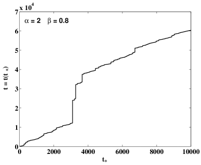
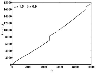
Figure 1: A sample path for ($rw_{1}$), the leading process $t=t(t_{*})$.

LEFT: $\{\alpha=2\,,\;\beta=0.80\}$, RIGHT: $\{\alpha=1.5\,,\;\beta=0.90\}$.

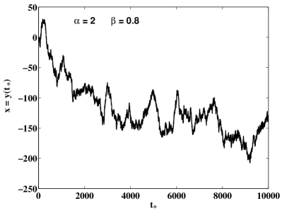
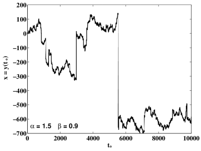
Figure 2: A sample path for ($rw_{2}$), the parent process $x=y(t_{*})$.

LEFT: $\{\alpha=2\,,\;\beta=0.80\}$, RIGHT: $\{\alpha=1.5\,,\;\beta=0.90\}$.

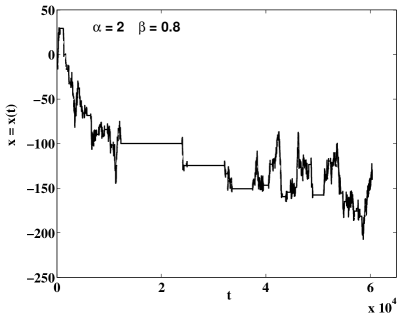
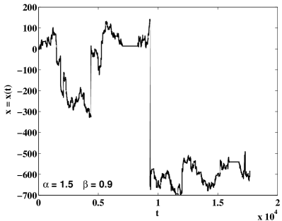
Figure 3: A sample path for ($rw$), the subordinated process $x=x(t)$.

LEFT: $\{\alpha=2\,,\;\beta=0.80\}$, RIGHT: $\{\alpha=1.5\,,\;\beta=0.90\}$.

Plots in Fig. 1 (devoted to the leading process, the limit of ($rw_{1}$)) thus represent sample paths in the $(t_{*},t)$ plane of unilateral Lévy motions of order $\beta$. By interchanging the coordinate axes we can consider Fig 1 as representing sample paths of the directing process, the limit of ($rw_{3}$).

Plots in Fig. 2 (devoted to the parent process, the limit of ($rw_{2}$)) represent sample paths in the $(t_{*},x)$ plane, produced in the way explained above, for Lévy motions of order $\alpha$ and skewness $\theta=0$ (symmetric stable distributions). As indicated above, it is possible to produce $10000$ independent identically distributed random deviates, say $T_{1},T_{2},\dots,T_{10000}$ having a stable probability distribution with order $\beta$ and skewness $-\beta$ (extremal stable distributions). Then, consider the points

$$t_{0}=0,\quad t_{n}=\sum\limits_{k=1}^{n}T_{k},\quad n\geq 1\,,$$

and plot the couples $(t_{*,n},t_{n})$ in the $(t_{*},t)$ (operational time, physical time) plane. By connecting points with horizontal and vertical lines we get sample paths $\{t(t_{*}):0\leq t_{*}\leq 10000\}$ describing the evolution of the physical time $t$ with the increasing of the operational time $t_{*}.$ Now, plotting points $(t(t_{*,n}),y(t_{*,n}))$ in the $(t,x)$ plane, namely the physical time-space plane, and connecting them as before, one gets a good approximation of the sample paths of the subordinated fractional diffusion process of parameters $\alpha$, $\beta$ and $\theta=0$.

In Fig. 3 (devoted to the subordinated process, the limit of ($CTRW$)) we show paths obtained in this way, from the points calculated in the previous paths. In Fig.3 Left we plotted the points $(t(t_{*,n}),y(t_{*,n}))$ obtained in Fig. 1 Left and Fig. 2 Left, while Fig.3 Right shows the points of Fig. 1 Right and Fig. 2 Right.

By observing the figures the reader will note that horizontal segments (waiting times) in the $(t,x)$ plane (Fig. 3) correspond to vertical segments (jumps) in the $(t,t_{*})$ plane (Fig. 1). Actually, the graphs in the $(t,x)$-plane depict continuous time random walks with waiting times $T_{k}$ (shown as horizontal segments) and jumps $X_{k}$ (shown as vertical segments). The left endpoints of the horizontal segments can be considered as snapshots of the true particle path (the true random process to be simulated), the segments being segments of our ignorance. In the interval $t_{n}<t\leq t_{n+1}$ the true process (namely the spatial variable $x=X(t)$) may jump up and down (infinitely) often, the sum (or integral) of all these ups (counted positive) and downs (counted negative) amounting to the vertical jump $X_{n+1}$. Finer details will become visible by choosing in the operational time $t_{*}$ the step length $\tau<<1$ (instead of length 1 as we have done) and correspondingly the waiting times and spatial jumps as $\tau^{1/\beta}$ multiplied by a standard extreme $\beta$-stable deviate, $\tau^{1/\alpha}$ multiplied by a standard (in our special case: symmetric) $\alpha$-stable deviate, respectively, as required by the self-similarity properties of the stable probability distributions. In a forthcoming paper we will describe in detail what happens for finer and finer discretization of the operational time $t_{*}$.

9. Conclusions

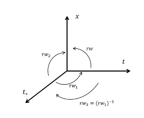
Figure 4: Diagram for the connections between the four random walks ($rw_{1}$), ($rw_{2}$),($rw_{3}$) and ($CTRW$)=($rw$).

After sketching our method of well-scaled transition to the diffusion limit under power law regime, we have slpitted the $CTRW$ into three random walks($rw_{1}$), ($rw_{2}$), ($rw_{3}$), each of them involving two of the three directions: natural time, operational time and space. The random walk ($rw_{3}$) is the inverse of ($rw_{1}$). To better visualize the matter, here Fig. 4 shows in form of a diagram the connections between the three random walks ($rw_{1}$), ($rw_{2}$), ($rw_{3}$) and ($rw$) $\,\equiv\,$ ($CTRW$).

In section 8 the figures 1, 2, 3 have shown some numerical realizations of these random walks. We can consider Fig. 1 as a representation of ($rw_{1}$), or by interchange of axes as one of ($rw_{3}$), Fig. 2 as one of ($rw_{2}$), and finally Fig. 3 as a representation of ($CTRW$).

We have carried out the analysis of transition by aid of the transforms of Fourier and Laplace, thereby consistently using corresponding variants of the Montroll-Weiss equation (not only in space and natural time, but also not conventionally in the above-mentioned combinations). In this way we have exhibited the true power of this equation in asymptotic analysis of random walks. In a quite natural way we have interpreted the diffusion limits as leading to the common subordination formula as well as the method of parametric subordination of constructing trajectories of particles.

Acknowledgments

We gratefully appreciate helpful comments of our colleague Enrico Scalas to a draft of this paper.

References

1. E. Barkai, Fractional Fokker-Planck equation, solution, and application, Phys. Rev. E 63, 046118-1/18 (2001).

2. P. Butzer, U. Westphal, Introduction to fractional calculus, in: H. Hilfer (Editor), Fractional Calculus, Applications in Physics (World Scientific, Singapore, 2000), pp. 1–85.

3. W. Feller, An Introduction to Probability Theory and its Applications, Vol II (Wiley, New York, 1971).

4. H.C. Fogedby, Langevin equations for continuous time Lévy flights, Phys. Rev. E 50, 1657–1660 (1994).

5. D. Fulger, E. Scalas, G. Germano, Monte Carlo simulation of uncoupled continuous-time random walks yielding a stochastic solution of the space-time fractional diffusion equation. Phys. Rev. E 77, 021122/1–7 (2008).

6. G. Germano, M. Politi, E. Scalas, R.L. Schilling, Stochastic calculus for uncoupled continuous-time random walks. Phys. Rev. E 79, 066102/1–12 (2009).

7. R. Gorenflo, Mittag-Leffler waiting time, power laws, rarefaction, continuous time random walk, diffusion limit, in S.S. Pai, N. Sebastian, S.S. Nair, D.P. Joseph and D. Kumar (Editors), Proceedings of the National Workshop on Fractional Calculus and Statistical Distributions, (CMS Pala Campus, India, 2010), pp. 1–22. [E-print: http://arxiv.org/abs/1004.4413]

8. R. Gorenflo, F. Mainardi, Fractional calculus: integral and differential equations of fractional order, in: A. Carpinteri and F. Mainardi (Editors), Fractals and Fractional Calculus in Continuum Mechanics (Springer Verlag, Wien 1997), pp. 223–276. [E-print: http://arxiv.org/abs/0805.3823]

9. R. Gorenflo, F. Mainardi, Fractional diffusion processes: probability distributions and continuous time random walk, in: G. Rangarajan and M. Ding (Editors), Processes with Long Range Correlations (Springer-Verlag, Berlin, 2003), pp. 148–166. [E-print: http://arxiv.org/abs/0709.3990]

10. R. Gorenflo, F. Mainardi, Continuous time random walk, Mittag-Leffler waiting time and fractional diffusion: mathematical aspects, in: R. Klages, G. Radons, and I.M. Sokolov, (Editors), Anomalous Transport, Foundations and Applications (Wiley-VCH Verlag, Weinheim, Germany, 2008), pp. 93–127. [E-print: arXiv:cond-mat/07050797]

11. R. Gorenflo, F. Mainardi, A. Vivoli, Continuous time random walk and parametric subordination in fractional diffusion, Chaos, Solitons and Fractals 34, 87–103 (2007). [E-print http://arxiv.org/abs/cond-mat/0701126]

12. R. Hilfer, Threefold introduction to fractional calculus, in R. Klages, G. Radons and I.M. Sokolov (Editors), Anomalous Transport, Foundations and Applications (Wiley-VCH Verlag, Weinheim, Germany, 2008), pp. 17–73.

13. R. Hilfer, Exact solutions for a class of fractal time random walks, Fractals 3, 211-216 (1995).

14. R. Hilfer, L. Anton, Fractional master equations and fractal time random walks, Phys. Rev. E 51, R848–R851 (1995).

15. A.A. Kilbas, H.M. Srivastava, J.J. Trujillo, Theory and Applications of Fractional Differential Equations (Elsevier, Amsterdam, 2006).

16. D. Kleinhans, R. Friedrich, Continuous-time random walks: Simulations of continuous trajectories, Phys. Rev E 76, 061102/1–6 (2007).

17. F. Mainardi, Fractional Calculus and Waves in Linear Viscoelasticity (Imperial College Press, London, 2010).

18. F. Mainardi, Yu. Luchko, G. Pagnini, The fundamental solution of the space-time fractional diffusion equation, Fract. Calculus and Appl. Analysis 4, 153–192 (2001). [E-print: http://arxiv.org/abs/cond-mat/0702419]

19. F. Mainardi, G. Pagnini, R.K. Saxena, Fox $H$ functions in fractional diffusion, J. Computational and Appl. Mathematics 178, 321–331 (2005).

20. A.M Mathai, R.K. Saxena, H.J Haubold, The H-function, Theory and Applications (Springer Verlag, New York, 2010).

21. M.M. Meerschaert, D.A. Benson, H.P Scheffler, B. Baeumer, Stochastic solutions of space-fractional diffusion equation, Phys. Rev. E 65, 041103/1–4 (2002).

22. M.M. Meerschaert, H.P Scheffler, Limit theorems for continuous-time random walks with infinite mean waiting times, J. Appl. Prob. 41, 623–638 (2004).

23. R. Metzler, J. Klafter, The restaurant at the end of the random walk: Recent developments in the description of anomalous transport by fractional dynamics, J. Phys. A. Math. Gen. 37, R161–R208 (2004).

24. I. Podlubny, Fractional Differential Equations (Academic Press, San Diego, 1999).

25. B. Rubin, Fractional Integrals and Potentials (Addison-Wesley & Longman, Harlow, 1996).

26. S.G. Samko, A.A. Kilbas, O.I. Marichev, Fractional Integrals and Derivatives: Theory and Applications (Gordon and Breach, New York, 1993).

27. E. Scalas, R. Gorenflo, F. Mainardi, Uncoupled continuous-time random walks: Solution and limiting behavior of the master equation, Phys. Rev. E 69, 011107/1–8 (2004).

28. Z. Tomovski, R. Hilfer, H.M. Srivastava, Fractional and operational calculus with generalized fractional derivative operators and Mittag-Leffler type functions, Integral Transforms Spec. Funct. 21, 797– 814 (2010).

29. G.H. Weiss, Aspects and Applications of Random Walks (North-Holland, Amsterdam, 1994).

30. Y. Zhang, M.M. Meerschaert, B. Baeumer, Particle tracking for time-fractional diffusion, Phys. Rev. E. 78, 036705/1–7 (2008).