Testing the Equality of Covariance Operators in Functional Samples

STEFAN FREMDT
Mathematical Institute, University of Cologne

LAJOS HORVÁTH
Department of Mathematics, University of Utah

PIOTR KOKOSZKA
Department of Mathematics and Statistics, Utah State University

JOSEF G. STEINEBACH
Mathematical Institute, University of Cologne

ABSTRACT.

We propose a robust test for the equality of the covariance structures in two functional samples. The test statistic has a chi-square asymptotic distribution with a known number of degrees of freedom, which depends on the level of dimension reduction needed to represent the data. Detailed analysis of the asymptotic properties is developed. Finite sample performance is examined by a simulation study and an application to egg–laying curves of fruit flies. Keywords: Asymptotic distribution, Covariance operator, Functional data, Quadratic forms, Two sample problem. Abbreviated Title: Equality of covariance operators AMS subject classification: Primary 62G10; secondary 62G20, 62H15

1. Introduction

The last decade has seen increasing interest in methods of functional data analysis which offer novel and effective tools for dealing with problems where curves can naturally be viewed as data objects. The books by Ramsay & Silverman (2005) and Ramsay et al. (2009) offer comprehensive introductions to the subject, the collection Ferraty & Romain (2011) reviews some recent developments focusing on advances in the relevant theory, while the monographs of Bosq (2000), Ferraty & Vieu (2006) and Horváth & Kokoszka (2011+) develop the field in several important directions. Despite the emergence of many alternative ways of looking at functional data, and many dimension reduction approaches, the functional principal components (FPC’s) still remain the most important starting point for many functional data analysis procedures, Reiss & Ogden (2007), Gervini (2008), Yao & Müller (2010), Gabrys et al. (2010) are just a handful of illustrative references. The FPC’s are the eigenfunctions of the covariance operator. This paper focuses on testing if the covariance operators of two functional samples are equal. By the Karhunen-Loève expansion, this is equivalent to testing if both samples have the same set of FPC’s. Benko et al. (2009) developed bootstrap procedures for testing the equality of specific FPC’s. Panaretos et al. (2010) proposed a test of the type we consider, but assuming that the curves have a Gaussian distribution. The main result of Panaretos et al. (2010) follows as a corollary of our more general approach (Theorem 2).

Despite their importance, two sample problems for functional data received relatively little attention. In addition to the work of Benko et al. (2009) and Panaretos et al. (2010), the relevant references are Horváth et al. (2009) and Horváth et al. (2011) who focus, respectively, on the regression kernels in functional linear models and the mean of functional data exhibiting temporal dependence. Clearly, if some population parameters of two functional samples are different, estimating them using the pooled sample may lead to spurious conclusions. Due to the importance of the FPC’s, a relatively simple and robust procedure for testing the equality of the covariance operators is called for.

The remainder of this paper is organized as follows. Section 2. sets out the notation and definitions. The construction of the test statistic and its asymptotic properties are developed in Section 3.. Section 4. reports the results of a simulation study and illustrates the procedure by application to egg-laying curves of Mediterranean fruit flies. The proofs of the asymptotic results of Section 3. are given in Section 5..

2. Preliminaries

Let $X_{1},X_{2},\ldots,X_{N}$ be independent, identically distributed random variables in $L_{2}[0,1]$ with $EX_{i}(t)=\mu(t)$ and $cov(X_{i}(t),X_{i}(s))=C(t,s)$. We assume that another sample $X^{\ast}_{1},X^{\ast}_{2},\ldots X^{\ast}_{M}$ is also available and let $\mu^{\ast}(t)=EX^{\ast}_{i}(t)$ and $C^{\ast}(t,s)=cov(X^{\ast}_{i}(t),X^{\ast}_{i}(s))$ for $t,s\in[0,1].$ We wish to test the null hypothesis

$$H_{0}:~{}C=C^{\ast}$$

against the alternative $H_{A}$ that $H_{0}$ does not hold.

A crucial assumption considering the asymptotics of our test procedure will be that

$$\Theta_{N,M}=\frac{N}{M+N}\to\Theta\in(0,1)\quad\text{as}\quad N,M\to\infty.$$ (1)

For the construction of our test procedure we will use an estimate of the asymptotic pooled covariance operator $\mathfrak{R}$ of the two given samples (cf. (4)) which is defined by the kernel

$$R(t,s)=\Theta C(t,s)+(1-\Theta)C^{\ast}(t,s).$$

Denote by $(\lambda_{1},\varphi_{1}),(\lambda_{2},\varphi_{2}),\ldots$ the eigenvalue/eigenfunction pairs of $\mathfrak{R}$, which are defined by

$$\lambda_{k}\varphi_{k}(t)=\mathfrak{R}\varphi_{k}(t)=\int^{1}_{0}R(t,s)\varphi_{k}(s)ds,\quad t\in[0,1],\quad 1\leq k<\infty~{}.$$ (2)

Throughout this paper we assume

$$\lambda_{1}>\lambda_{2}>\ldots>\lambda_{p}>\lambda_{p+1},$$ (3)

i.e. there exist at least $p$ distinct (positive) eigenvalues. Under assumption (3), we can uniquely (up to signs) choose $\varphi_{1},\ldots,\varphi_{p}$ satisfying (2), if we require $\|\varphi_{i}\|=1$, where for a positive integer $d$ and for $x\in L_{2}\left([0,1]^{d}\right)$

$$\|x\|=\left(\int^{1}_{0}\cdots\int^{1}_{0}x^{2}(t_{1},\ldots,t_{d})dt_{1}\cdots dt_{d}\right)^{1/2}.$$

Thus, under (3), $\{\varphi_{i},1\leq i\leq p\}$ is an orthonormal system that can be extended to an orthonormal basis $\{\varphi_{i},1\leq i<\infty\}$.

If $H_{0}$ holds, then $(\lambda_{i},\varphi_{i}),~{}1\leq i<\infty,$ are also the eigenvalues/eigenfunctions of the covariance operators $\mathfrak{C}$ of the first and $\mathfrak{C}^{\ast}$ of the second sample. To construct a test statistic which converges under $H_{0}$, we can therefore pool the two samples, as explained in Section 3..

3. The test and the asymptotic results

Our procedure is based on projecting the observations onto a suitably chosen finite-dimensional space. To define this space, introduce the empirical pooled covariance operator $\widehat{\mathfrak{R}}_{N,M}$ defined by the kernel

$$\widehat{R}_{N,M}(t,s)=\frac{1}{N+M}\Biggl{\{} \mathop{\sum}\limits^{N}_{k=1}(X_{k}(t)-\overline{X}_{N}(t))(X_{k}(s)-\overline{X}_{N}(s))$$ (4)

$$+\mathop{\sum}\limits^{M}_{k=1}(X^{\ast}_{k}(t)-\overline{X}_{M}^{*}(t))(X^{\ast}_{k}(s)-\overline{X}_{M}^{*}(s))\Biggr{\}},$$

where

$$\overline{X}_{N}(t)=\frac{1}{N}\mathop{\sum}\limits^{N}_{k=1}X_{k}(t)\quad\hbox{and}\quad\overline{X}^{\ast}_{M}(t)=\frac{1}{M}\sum^{M}_{k=1}X^{\ast}_{k}(t)$$

are the sample mean functions. Let $(\widehat{\lambda}_{i},\widehat{\varphi}_{i})$ denote the eigenvalues/eigenfunctions of $\widehat{\mathfrak{R}}_{N,M}$, i.e.

$$\widehat{\lambda}_{i}\widehat{\varphi}_{i}(t)=\widehat{\mathfrak{R}}_{N,M}\widehat{\varphi}_{i}(t)=\mathop{\int}\limits^{1}_{0}\widehat{R}_{N,M}(t,s)\widehat{\varphi}_{i}(s)ds,\quad t\in[0,1],\quad 1\leq i\leq N+M,$$

with $\widehat{\lambda}_{1}\geq\widehat{\lambda}_{2}\geq\ldots~{}.$ We can and will assume that the $\widehat{\varphi}_{i}$ form an orthonormal system. We consider the projections

$$\widehat{a}_{k}(i)=\langle X_{k}-\overline{X}_{N},\widehat{\varphi}_{i}\rangle=\mathop{\int}\limits^{1}_{0}(X_{k}(t)-\overline{X}_{N}(t))\widehat{\varphi}_{i}(t)dt$$ (5)

and

$$\widehat{a}^{\ast}_{k}(j)=\langle X^{\ast}_{k}-\overline{X}^{\ast}_{M},\widehat{\varphi}_{j}\rangle=\mathop{\int}\limits^{1}_{0}\left(X^{\ast}_{k}(t)-\overline{X}^{\ast}_{M}(t)\right)\widehat{\varphi}_{j}(t)dt.$$ (6)

To test $H_{0}$, we compare the matrices $\widehat{\Delta}_{N}$ and $\widehat{\Delta}^{\ast}_{M}$ with entries

$$\widehat{\Delta}_{N}(i,j)=\frac{1}{N}\mathop{\sum}\limits^{N}_{k=1}\widehat{a}_{k}(i)\widehat{a}_{k}(j),\quad 1\leq i,j\leq p,$$

and

$$\widehat{\Delta}^{\ast}_{M}(i,j)=\frac{1}{M}\mathop{\sum}\limits^{M}_{k=1}\widehat{a}^{\ast}_{k}(i)\widehat{a}^{\ast}_{k}(j),\quad 1\leq i,j\leq p.$$

We note that $\widehat{\Delta}_{N}(i,j)-\widehat{\Delta}^{\ast}_{M}(i,j)$ is the projection of $\widehat{C}_{N}(t,s)-\widehat{C}^{\ast}_{M}(t,s)$ in the direction of $\widehat{\varphi}_{i}(t)\widehat{\varphi}_{j}(s)$, where

$$\widehat{C}_{N}(t,s)=\frac{1}{N}\mathop{\sum}\limits^{N}_{k=1}\left(X_{k}(t)-\overline{X}_{N}(t)\right)\left(X_{k}(s)-\overline{X}_{N}(s)\right)$$

and

$$\widehat{C}^{\ast}_{M}(t,s)=\frac{1}{M}\mathop{\sum}\limits^{M}_{k=1}\left(X^{\ast}_{k}(t)-\overline{X}^{\ast}_{M}(t)\right)\left(X^{\ast}_{k}(s)-\overline{X}^{\ast}_{M}(s)\right)$$

are the empirical covariances of the two samples.

From the columns below the diagonal of $\widehat{\Delta}_{N}-\widehat{\Delta}^{\ast}_{M}$ we create a vector $\widehat{\boldsymbol{\xi}}_{N,M}$ as follows:

$$\widehat{\boldsymbol{\xi}}_{N,M}=\mbox{vech}\left(\widehat{\Delta}_{N}-\widehat{\Delta}^{\ast}_{M}\right)=\left(\begin{array}[]{c}\widehat{\Delta}_{N}(1,1)-\widehat{\Delta}^{\ast}_{M}(1,1)\\ \widehat{\Delta}_{N}(2,1)-\widehat{\Delta}^{\ast}_{M}(2,1)\\ \vdots\\ \widehat{\Delta}_{N}(p,p)-\widehat{\Delta}^{\ast}_{M}(p,p)\end{array}\right).$$ (11)

For the properties of the vech operator we refer to Abadir & Magnus (2005).
Next we estimate the asymptotic covariance matrix of $(MN/(N+M))^{1/2}\widehat{\boldsymbol{\xi}}_{N,M}.$ Let

$$\widehat{L}_{N,M}(k,k^{\prime})= \left(1-\Theta_{N,M}\right)\left\{\frac{1}{N}\mathop{\sum}\limits^{N}_{\ell=1}\widehat{a}_{\ell}(i)\widehat{a}_{\ell}(j)\widehat{a}_{\ell}(i^{\prime})\widehat{a}_{\ell}(j^{\prime})-\big{\langle}\widehat{\mathfrak{C}}_{N}\widehat{\varphi}_{i},\widehat{\varphi}_{j}\big{\rangle}\big{\langle}\widehat{\mathfrak{C}}_{N}\widehat{\varphi}_{i^{\prime}},\widehat{\varphi}_{j^{\prime}}\big{\rangle}\right\}$$

$$+\Theta_{N,M}\left\{\frac{1}{M}\mathop{\sum}\limits^{M}_{\ell=1}\widehat{a}^{\ast}_{\ell}(i)\widehat{a}^{\ast}_{\ell}(j)\widehat{a}^{\ast}_{\ell}(i^{\prime})\widehat{a}^{\ast}_{\ell}(j^{\prime})-\big{\langle}\widehat{\mathfrak{C}}^{\ast}_{M}\widehat{\varphi}_{i},\widehat{\varphi}_{j}\big{\rangle}\big{\langle}\widehat{\mathfrak{C}}^{\ast}_{M}\widehat{\varphi}_{i^{\prime}},\widehat{\varphi}_{j^{\prime}}\big{\rangle}\right\}$$

where $i,j,i^{\prime},j^{\prime}$ depend on $k,k^{\prime}$ (see below), and $\widehat{\mathfrak{C}}_{N}$ $(\widehat{\mathfrak{C}}^{\ast}_{M})$ is interpreted as an operator with $\widehat{\mathfrak{C}}_{N}$ defined as

$$\widehat{\mathfrak{C}}_{N}\widehat{\varphi}_{i}=\int^{1}_{0}\widehat{C}_{N}(t,s)\widehat{\varphi}_{i}(s)ds.$$

(An analogous definition holds for $\widehat{\mathfrak{C}}^{\ast}_{M}$.) From this definition it follows that

$$\big{\langle}\widehat{\mathfrak{C}}_{N}\widehat{\varphi}_{i},\widehat{\varphi}_{j}\big{\rangle}=\frac{1}{N}\mathop{\sum}\limits^{N}_{l=1}\widehat{a}_{\ell}(i)\widehat{a}_{\ell}(j).$$

We note that one can use $\widehat{L}^{\ast}_{N,M}(k,k^{\prime})$ instead of $\widehat{L}_{N,M}(k,k^{\prime}),$ where $\widehat{L}^{\ast}_{N,M}(k,k^{\prime})$ is defined like $\widehat{L}_{N,M}(k,k^{\prime}),$ but $\big{\langle}\widehat{\mathfrak{C}}_{N}\widehat{\varphi}_{i},\widehat{\varphi}_{j}\big{\rangle}$ and $\big{\langle}\widehat{\mathfrak{C}}^{\ast}_{M}\widehat{\varphi}_{i},\widehat{\varphi}_{j}\big{\rangle}$ are replaced with $0$ if $i\neq j$ and $\widehat{\lambda}_{i}$ if $i=j.$ In the same spirit, $\big{\langle}\widehat{\mathfrak{C}}_{N}\widehat{\varphi}_{i^{\prime}},\widehat{\varphi}_{j^{\prime}}\big{\rangle}$ and $\big{\langle}\widehat{\mathfrak{C}}^{\ast}_{M}\widehat{\varphi}_{i^{\prime}},\widehat{\varphi}_{j^{\prime}}\big{\rangle}$ are replaced with $0$ for ${i^{\prime}}\neq{j^{\prime}}$ and $\widehat{\lambda}_{i^{\prime}}$ if ${i^{\prime}}={j^{\prime}}.$

The index $(i,j)$ is computed from $k$ in the following way: Let

$$k^{\prime}=\frac{p(p+1)}{2}-k+1,\quad i^{\prime}=p-i+1,\quad\mbox{and}\quad j^{\prime}=p-j+1.$$ (12)

We look at an upper triangle matrix $(a_{i^{\prime},j^{\prime}})$. Then, for column $j^{\prime},$ we have that $(j^{\prime}-1)j^{\prime}/2<k\leq j^{\prime}(j^{\prime}+1)/2.$ Thus $j^{\prime}=\left\lceil\sqrt{2k^{\prime}+\frac{1}{4}}-\frac{1}{2}\right\rceil$ and $i^{\prime}=k^{\prime}-(j^{\prime}-1)j^{\prime}/2,$ where $\lceil r\rceil=\min\{k\in\mathbb{Z}:\,k\geq r\}$ for $r\in\mathbb{R}.$ Consequently, the index $(i,j)$ can be computed from $k$ via

$$j=p-\left\lceil\sqrt{p(p+1)-2k+\frac{9}{4}}-\frac{1}{2}\right\rceil+1\quad\mbox{and}\quad i=k+p-p\cdot j+\frac{j(j-1)}{2}.$$ (13)

With the above notation, we can formulate the main result of this paper:

Theorem 1.

We assume that $H_{0}$, (1) and (3) hold, and

$$\int^{1}_{0}E(X_{1}(t))^{4}dt<\infty,\quad\int^{1}_{0}E(X^{\ast}_{1}(t))^{4}dt<\infty.$$ (14)

Then

$$\frac{NM}{N+M}\widehat{\boldsymbol{\xi}}^{T}_{N,M}\widehat{L}^{-1}_{N,M}\widehat{\boldsymbol{\xi}}_{N,M}~{}\mathop{\longrightarrow}\limits^{\mathcal{D}}~{}\chi^{2}_{p(p+1)/2},\quad\text{as}\quad N,M\to\infty,$$

where $\chi^{2}_{p(p+1)/2}$ stands for a $\chi^{2}$ random variable with $p(p+1)/2$ degrees of freedom.

Theorem 1 implies that the null hypothesis is rejected if the test statistic

$$\widehat{T}_{1}=\frac{NM}{N+M}\widehat{\boldsymbol{\xi}}^{T}_{N,M}\widehat{L}^{-1}_{N,M}\widehat{\boldsymbol{\xi}}_{N,M}$$

exceeds a critical quantile of the chi–square distribution with $p(p+1)/2$ degrees of freedom.

If both samples are Gaussian random processes, the quadratic form $\widehat{\boldsymbol{\xi}}^{T}_{N,M}\widehat{L}_{N,M}^{-1}\widehat{\boldsymbol{\xi}}_{N,M}$ can be replaced with the normalized sum of the squares of $\widehat{\Delta}_{N,M}(i,j)-\widehat{\Delta}^{\ast}_{N,M}(i,j)$, as stated in the following theorem.

Theorem 2.

If $X_{1},X^{\ast}_{1}$ are Gaussian processes and the conditions of Theorem 1 are satisfied, then, as $N,M\to\infty$,

$$\widehat{T}_{2}=\frac{NM}{N+M}\mathop{\sum}\limits_{1\leq i,j\leq p}\frac{1}{2}\frac{\left(\widehat{\Delta}_{N,M}(i,j)-\widehat{\Delta}^{\ast}_{N,M}(i,j)\right)^{2}}{\widehat{\lambda}_{i}\widehat{\lambda}_{j}}~{}\mathop{\longrightarrow}\limits^{\mathcal{D}}~{}\chi^{2}_{p(p+1)/2}.$$

Observe that the statistic $\widehat{T}_{2}$ can be written as

$$\widehat{T}_{2}=\frac{NM}{N+M}\left\{\mathop{\sum}\limits_{1\leq i<j\leq p}\frac{\left(\widehat{\Delta}_{N,M}(i,j)-\widehat{\Delta}^{\ast}_{N,M}(i,j)\right)^{2}}{\widehat{\lambda}_{i}\widehat{\lambda}_{j}}+\mathop{\sum}\limits^{p}_{i=1}\frac{\left(\widehat{\Delta}_{N,M}(i,i)-\widehat{\Delta}^{\ast}_{N,M}(i,i)\right)^{2}}{2\widehat{\lambda}_{i}^{2}}\right\}.$$

Next we discuss the asymptotic consistency of the testing procedure based on Theorem 1. Analogously to the definition of $\widehat{\boldsymbol{\xi}}_{N,M}$ we define the vector $\boldsymbol{\xi}=(\xi(1),\ldots,\xi(p(p+1)/2))$ using the columns of the matrix

$$\boldsymbol{D}=\left(\mathop{\int}\limits_{0}^{1}\mathop{\int}\limits_{0}^{1}(C(t,s)-C^{\ast}(t,s))\varphi_{i}(t)\varphi_{j}(s)dt\,ds\right)_{i,j=1,\ldots,p}$$ (15)

instead of $\widehat{\Delta}_{N}-\widehat{\Delta}^{\ast}_{M}$, i.e.

$$\widehat{\boldsymbol{\xi}}=\mbox{vech}(\boldsymbol{D}).$$

Theorem 3.

We assume that $H_{A}$, (1), (3) and (14) hold. Then there exist random variables $\widehat{h}_{1}=\widehat{h}_{1}(N,M),\ldots,\widehat{h}_{p(p+1)/2}=\widehat{h}_{p(p+1)/2}(N,M)$, taking values in $\{-1,1\}$ such that, as $N,M\to\infty$,

$$\max_{1\leq i\leq p(p+1)/2}\left|\widehat{\xi}_{N,M}(i)-\widehat{h}_{i}\xi(i)\right|=o_{P}(1)$$ (16)

and therefore

$$\left|\widehat{\boldsymbol{\xi}}_{N,M}\right|\mathop{\to}\limits^{P}\left|\boldsymbol{\xi}\right|,$$ (17)

where $|\cdot|$ denotes the Euclidean norm. If $\boldsymbol{\xi}\neq\mathbf{0}$ and the $p$ largest eigenvalues of $C$ and $C^{\ast}$ are positive, we also have

$$\widehat{T}_{1}\mathop{\to}\limits^{P}\infty,\quad\text{as}\quad N,M\to\infty.$$ (18)

The assumption that the $p$ largest eigenvalues of $C$ and $C^{\ast}$ are positive implies that the random functions $X_{i},~{}i=1,\ldots,N$, and $X^{\ast}_{j},~{}j=1,\ldots,M$, are not included in a $(p-1)$-dimensional subspace.

The application of the test requires the selection of the number $p$ of the empirical FPC’s to be used. A rule of thumb is to choose $p$ so that the first $p$ empirical FPC’s in each sample (i.e. those calculated as the eigenfunctions of $\widehat{C}_{N}$ and $\widehat{C}^{\ast}_{M}$) explain about 85–90% of the variance in each sample. Choosing $p$ too large generally negatively affects the finite sample performance of tests of this type, and for this reason we do not study asymptotics as $p$ tends to infinity. It is often illustrative to apply the test for a range of the values of $p$; each $p$ specifies a level of relevance of differences in the curves or kernels. A good practical approach is to look at the Karhunen–Loève approximations of the curves in both samples, and choose $p$ which gives approximation errors that can be considered unimportant.

4. A simulation study and application to medfly data

We first describe the results of a simulations study designed to evaluate finite sample properties of the tests based on the statistics $\widehat{T}_{1}$ and $\widehat{T}_{2}$. The emphasis is on the robustness to the violation of the assumption of normality. We simulated Gaussian curves as Brownian motions and Brownian bridges, and non–Gaussian curves via

$$Z_{n}(t)=A_{n}\sin(\pi t)+B_{n}\sin(2\pi t)+C_{n}\sin(4\pi t),$$ (19)

where $A_{n}=5Y_{1}$, $B_{n}=3Y_{2}$, $C_{n}=Y_{3}$ and $Y_{1},Y_{2},Y_{3}$ are independent $t_{5}$-distributed random variables. All curves were simulated at 1000 equidistant points in the interval $[0,1]$, and transformed into functional data objects using the Fourier basis with 49 basis functions. For each data generating process we used one thousand replications.

Table 1: Empirical sizes of the tests based on statistics $\widehat{T}_{1}$ and $\widehat{T}_{2}$ for non–Gaussian data. The curves in each sample were generated according to (19).

	$p=2$
	$\widehat{T}_{1}$			$\widehat{T}_{2}$
Sample Sizes	1%	5%	10%	1%	5%	10%
$N=M=100$	0.005	0.028	0.061	0.152	0.275	0.380
$N=M=200$	0.003	0.021	0.058	0.163	0.314	0.402
$N=M=1000$	0.002	0.021	0.056	0.190	0.313	0.426
	$p=3$
	$\widehat{T}_{1}$			$\widehat{T}_{2}$
Sample Sizes	1%	5%	10%	1%	5%	10%
$N=M=100$	0.004	0.028	0.065	0.167	0.332	0.434
$N=M=200$	0.004	0.024	0.064	0.194	0.338	0.423
$N=M=1000$	0.004	0.028	0.070	0.240	0.384	0.484

Table 1 displays the empirical sizes for non–Gaussian data. The test based on $\widehat{T}_{2}$ has severely inflated size, due to the violation of the assumption of normality. As documented in Panaretos et al. (2010), and confirmed by our own simulations, this test has very good empirical size when the data are Gaussian. The test based on $\widehat{T}_{1}$ is conservative, especially for smaller sample sizes. This is true for both Gaussian and non–Gaussian data; there is not much difference in the empirical size of this test for different data generating processes. Reflecting its conservative size, statistic $\widehat{T}_{1}$ leads to smaller power than $\widehat{T}_{2}$. We also studied a Monte Carlo version of the test based on the statistic $\widehat{T}_{3}={NM}(N+M)^{-1}\widehat{\boldsymbol{\xi}}^{T}_{N,M}\widehat{\boldsymbol{\xi}}_{N,M}$, and found that its finite sample properties were similar to those of the test based on $\widehat{T}_{1}$.

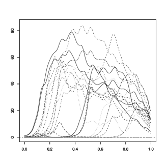
Figure 1: Ten randomly selected smoothed egg-laying curves of short-lived medflies (left panel), and ten such curves for long–lived medflies (right panel).

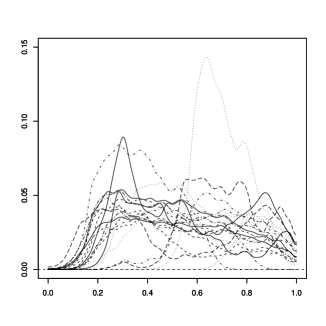
Figure 2: Ten randomly selected smoothed egg-laying curves of short-lived medflies (left panel), and ten such curves for long–lived medflies (right panel), relative to the number of eggs laid in the fly’s lifetime.

We now describe the results of the application of both tests to an interesting data set consisting of egg–laying trajectories of Mediterranean fruit flies (medflies). The data were kindly made available to us by Hans–Georg Müller. This data set has been extensively studied in biological and statistical literature, see Müller & Stadtmüller (2005) and references therein. We consider 534 egg-laying curves of medflies who lived at least 34 days. We examined two versions of these egg-laying curves, the functions in either version are defined over an interval $[0,30]$, and $t\leq 30$ is the day. Version 1 curves (denoted $X_{i}(t)$) are the absolute counts of eggs laid by fly $i$ on day $t$. Version 2 curves (denoted $Y_{i}(t)$) are the counts of eggs laid by fly $i$ on day $t$ relative to the total number of eggs laid in the lifetime of fly $i$. The 534 flies are classified into long-lived, i.e. those who lived 44 days or longer, and short-lived, i.e. those who died before the end of the 43rd day after birth. In the data set, there are 256 short-lived, and 278 long-lived flies. This classification naturally defines two samples: Sample 1: the egg-laying curves $\{X_{i}(t)($resp. $Y_{i}(t)),\ 0<t\leq 30,\ i=1,2,\ldots,256\}$ of the short-lived flies. Sample 2: the egg-laying curves $\{X_{j}^{*}(t)($resp. $Y_{j}^{*}(t)),\ 0<t\leq 30,\ j=1,2,\ldots,278\}$ of the long-lived flies. The egg-laying curves are very irregular; Figure 1 shows ten (smoothed) curves of short- and long-lived flies for version 1, Figure 2 shows ten (smoothed) curves for version 2 (both using a B-spline basis for the representation).

Figure 3: Normal QQ–plots for the scores of the version 2 medfly data with respect to the first two Fourier basis functions. Left – sample 1, Right – sample 2.

Table 2: P–values (in percent) of the test based on statistics $\widehat{T}_{1}$ and $\widehat{T}_{2}$ applied to absolute medfly data. Here $f_{p}$ denotes the fraction of the sample variance explained by the first $p$ FPCs, i.e. $f_{p}=(\sum_{k=1}^{p}\hat{\lambda}_{k})/(\sum_{k=1}^{N+M}\hat{\lambda}_{k})$.

P-values
$p$	2	3	4	5	6	7	8	9
$\widehat{T}_{1}$	82.70	36.22	30.59	63.84	37.71	39.03	33.77	34.77
$\widehat{T}_{2}$	0.54	0.13	0.11	0.12	0.02	0.00	0.00	0.00
$f_{p}$	72.93	78.36	81.87	83.94	85.62	87.08	88.49	89.72

Table 3: P–values (in percent) of the test based on statistics $\widehat{T}_{1}$ applied to relative medfly data; $f_{p}$ denotes the fraction of the sample variance explained by the first $p$ FPCs, i.e. $f_{p}=(\sum_{k=1}^{p}\hat{\lambda}_{k})/(\sum_{k=1}^{N+M}\hat{\lambda}_{k})$.

P-values
$p$	2	3	4	5	6	7	8
$\widehat{T}_{1}$	0.14	0.06	0.33	1.50	3.79	4.53	10.28
$f_{p}$	33.99	44.08	52.72	59.04	65.08	70.40	75.29
$p$	9	10	11	12	13	14	15
$\widehat{T}_{1}$	5.51	2.78	5.32	3.21	1.78	6.28	3.80
$f_{p}$	79.91	83.72	86.58	89.02	91.34	93.30	95.03

Table 2 shows the P–values for the absolute egg-laying counts (version 1). For the statistic $\widehat{T}_{1}$ the null hypothesis cannot be rejected irrespective of the choice of $p$. For the statistic $\widehat{T}_{2}$, the result of the test varies depending on the choice of $p$. As explained in Section 3., the usual recommendation is to use the values of $p$ which explain 85 to 90 percent of the variance. For such values of $p$, $\widehat{T}_{2}$ leads to a clear rejection. Since this test has however overinflated size, we conclude that there is little evidence that the covariance structures of version 1 curves for long– and short–lived flies are different. For the version 2 curves, the statistic $\widehat{T}_{2}$ yields P–values equal to zero (in machine precision), potentially indicating that the covariance structures for the short– and long–lived flies are different. The assumption of a normal distribution is however questionable, as the QQ-plots in Figure 3 show. These QQ-plots are constructed for the inner products $\langle Y_{i},e_{k}\rangle$ and $\langle Y_{i}^{*},e_{k}\rangle$, where the $Y_{i}$ are the curves from one of the samples (we cannot pool the data to construct QQ-plots because we test if the stochastic structures are different), and $e_{k}$ is the $k$th element of the Fourier basis. The normality of a functional sample implies the normality of all projections onto a complete orthonormal system . For $\langle X_{i},e_{k}\rangle$, the QQ-plots show a strong deviation from a straight line for some projections. Almost all projections $\langle Y_{i},e_{k}\rangle$ have QQ-plots indicating a strong deviation from normality. It is therefore important to apply the robust test based on the statistic $\widehat{T}_{1}$. The corresponding P–values for version 2 are displayed in Table 3. For most values of $p$, these P–values indicate the rejection of $H_{0}$. Many of them hover around the 5 percent level, but since the test is conservative, we can with confidence view them as favoring $H_{A}$.

The above application confirms the properties of the statistics established through the simulation study. It shows that while there is little evidence that the covariance structures for the absolute counts are different, there is strong evidence that they are different for relative counts.

5. Proofs of the results of Section 3.

The proof of Theorem 1 follows from several lemmas, which we establish first. We can and will assume without loss of generality that $\mu(t)=\mu^{\ast}(t)=0$ for all $t\in[0,1]$.

We will use the identity

$$\frac{1}{N^{1/2}}\mathop{\sum}\limits^{N}_{k=1}\left(X_{k}(t)-\overline{X}_{N}(t)\right)\left(X_{k}(s)-\overline{X}_{N}(s)\right)$$ (20)

$$=\frac{1}{N^{1/2}}\mathop{\sum}\limits^{N}_{k=1}X_{k}(t)X_{k}(s)-N^{1/2}\overline{X}_{N}(t)\overline{X}_{N}(s),$$

and an analogous identity for the second sample.

Our first lemma establishes bounds in probability which will often be used in the proofs.

Lemma 1.

Under the assumptions of Theorem 1, as $N,M\to\infty$,

$$\left\|N^{-1/2}\mathop{\sum}\limits^{N}_{k=1}\left\{X_{k}(t)X_{k}(s)-C(t,s)\right\}\right\|=O_{P}(1),$$ (21)

$$\left\|N^{1/2}\overline{X}_{N}(t)\right\|=O_{P}(1),$$ (22)

and

$$\left\|M^{-1/2}\mathop{\sum}\limits^{M}_{k=1}\left\{X^{\ast}_{k}(t)X^{\ast}_{k}(s)-C^{\ast}(t,s)\right\}\right\|=O_{P}(1),$$ (23)

$$\left\|M^{1/2}\overline{X}^{\ast}_{M}(t)\right\|=O_{P}(1).$$ (24)

Proof..

First we note that

$$E\int^{1}_{0}\int^{1}_{0}\left[\frac{1}{N^{\frac{1}{2}}}\mathop{\sum}\limits^{N}_{k=1}\left\{X_{k}(t)X_{k}(s)-C(t,s)\right\}\right]^{2}dt\,ds=\int^{1}_{0}\int^{1}_{0}E\left\{X_{1}(t)X_{1}(s)-C(t,s)\right\}^{2}dt\,ds,$$

so, by Markov’s inequality, we have

$$\left\|\frac{1}{N^{\frac{1}{2}}}\mathop{\sum}\limits^{N}_{k=1}\left\{X_{k}(t)X_{k}(s)-C(t,s)\right\}\right\|^{2}=O_{P}(1).$$

Similar arguments yield (22) – (24). ∎

The next lemma shows that the estimation of the mean functions, cf. the definition of the projections $\widehat{a}_{k}(i)$ and $\widehat{a}_{k}^{*}(j)$ in (5) and (6), has an asymptotically negligible effect.

Lemma 2.

Under the assumptions of Theorem 1, for all $1\leq i,j\leq p$, as $N,M\to\infty$,

$$N^{1/2}\widehat{\Delta}_{N}(i,j)=\frac{1}{N^{1/2}}\mathop{\sum}\limits^{N}_{k=1}\langle X_{k},\widehat{\varphi}_{i}\rangle\langle X_{k},\widehat{\varphi}_{j}\rangle+O_{P}\left(N^{-1/2}\right)$$

and

$$M^{1/2}\widehat{\Delta}^{\ast}_{M}(i,j)=\frac{1}{M^{1/2}}\mathop{\sum}\limits^{M}_{k=1}\langle X^{\ast}_{k},\widehat{\varphi}_{i}\rangle\langle X^{\ast}_{k},\widehat{\varphi}_{j}\rangle+O_{P}\left(M^{-1/2}\right).$$

Proof..

Using (20) and (22) we have by the Cauchy-Schwarz inequality,

$$\left|\int^{1}_{0}\int^{1}_{0}N^{1/2}\overline{X}_{N}(t)\overline{X}_{N}(s)\widehat{\varphi}_{i}(t)\widehat{\varphi}_{j}(s)dt\,ds\right|$$

$$=N^{-1/2}\left|\int^{1}_{0}N^{1/2}\overline{X}_{N}(t)\widehat{\varphi}_{i}(t)dt\right|\left|\int^{1}_{0}N^{1/2}\overline{X}_{N}(s)\widehat{\varphi}_{j}(s)ds\right|$$

$$\leq N^{-1/2}\left(\int^{1}_{0}\left(N^{1/2}\overline{X}_{N}(t)\right)^{2}dt\int^{1}_{0}\widehat{\varphi}^{2}_{i}(t)dt\right)^{1/2}\left(\int^{1}_{0}\left(N^{1/2}\overline{X}_{N}(s)\right)^{2}ds\int^{1}_{0}\widehat{\varphi}^{2}_{j}(s)ds\right)^{1/2}$$

$$=N^{-1/2}\int^{1}_{0}\left(N^{1/2}\overline{X}_{N}(t)\right)^{2}dt$$

$$=O_{P}\left(N^{-1/2}\right).$$

The second part can be proven in the same way. ∎

We now state bounds on the distances between the estimated and the population eigenvalues and eigenfunctions. These bounds are true under the null hypothesis, and extend the corresponding one sample bounds.

Lemma 3.

If the conditions of Theorem 1 are satisfied, then, as $N,M\to\infty$,

$$\mathop{\max}\limits_{1\leq i\leq p}|\widehat{\lambda}_{i}-\lambda_{i}|=O_{P}\left((N+M)^{-1/2}\right)$$

and

$$\mathop{\max}\limits_{1\leq i\leq p}\|\widehat{\varphi}_{i}-\widehat{c}_{i}\varphi_{i}\|=O_{P}\left((N+M)^{-1/2}\right),$$

where

$$\widehat{c}_{i}=\widehat{c}_{i}(N,M)={\rm sign}(\langle\widehat{\varphi}_{i},\varphi_{i}\rangle).$$

Proof..

It follows from (21) – (24) and the assumption $C=C^{\ast}$ that

$$\left\|\widehat{R}_{N,M}-C\right\|=O_{P}\left(\left(N^{1/2}+M^{1/2}\right)\Big{/}(N+M)\right),$$

and since $N^{1/2}+M^{1/2}\leq 2(N+M)^{1/2}$, the result follows from the corresponding one sample bounds, see e.g. Chapter 2 of Horváth & Kokoszka (2011+). ∎

Lemma 3 now allows us to replace the estimated eigenfunctions by their population counterparts. The random signs $\widehat{c}_{i}$ must appear in the formulation of Lemma 4, but they cancel in the subsequent results.

Lemma 4.

If the conditions of Theorem 1 are satisfied, then, for all $1\leq i,j\leq p$, as $N,M\to\infty$,

$$\left(\frac{NM}{N+M}\right)^{1/2}\left(\widehat{\Delta}_{N}(i,j)-\widehat{\Delta}^{\ast}_{M}(i,j)\right)$$

$$=\left(\frac{NM}{N+M}\right)^{1/2}\left\{\frac{1}{N}\mathop{\sum}\limits^{N}_{k=1}\langle X_{k},\widehat{c}_{i}\varphi_{i}\rangle\langle X_{k},\widehat{c}_{j}\varphi_{j}\rangle-\frac{1}{M}\mathop{\sum}\limits^{M}_{k=1}\langle X^{\ast}_{k},\widehat{c}_{i}\varphi_{i}\rangle\langle X^{\ast}_{k},\widehat{c}_{j}\varphi_{j}\rangle\right\}+o_{P}(1).$$

Proof..

We write

$$\frac{1}{N}\mathop{\sum}\limits^{N}_{k=1}\langle X_{k},\widehat{\varphi}_{i}\rangle\langle X_{k},\widehat{\varphi}_{j}\rangle-\int^{1}_{0}\int^{1}_{0}C(t,s)\widehat{\varphi}_{i}(t)\widehat{\varphi}_{j}(s)dt~{}ds$$

$$=N^{1/2}\int^{1}_{0}\int^{1}_{0}\left\{\frac{1}{N^{1/2}}\mathop{\sum}\limits^{N}_{k=1}\big{(}X_{k}(t)X_{k}(s)-C(t,s)\big{)}\right\}\widehat{\varphi}_{i}(t)\widehat{\varphi}_{j}(s)dt\,ds.$$

Using Lemmas 1 – 3 we get

$$\left|\int^{1}_{0}\int^{1}_{0}\left\{\frac{1}{N^{1/2}}\sum^{N}_{k=1}\big{(}X_{k}(t)X_{k}(s)-C(t,s)\big{)}\right\}\big{(}\widehat{\varphi}_{i}(t)\widehat{\varphi}_{j}(s)-\widehat{c}_{i}\varphi_{i}(t)\widehat{c}_{j}\varphi_{j}(s)\big{)}dt\,ds\right|$$

$$=\Bigg{|}\int^{1}_{0}\int^{1}_{0}\left\{\frac{1}{N^{1/2}}\sum^{N}_{k=1}\big{(}X_{k}(t)X_{k}(s)-C(t,s)\big{)}\right\}$$

$$\qquad\times\left\{\big{(}\widehat{\varphi}_{i}(t)-\widehat{c}_{i}\varphi_{i}(t)\big{)}\widehat{\varphi}_{j}(s)+\widehat{c}_{i}\varphi_{i}(t)\big{(}\widehat{\varphi}_{j}(s)-\widehat{c}_{j}\varphi_{j}(s)\big{)}\right\}dt\,ds\Bigg{|}$$

$$\leq\Bigg{(}\int^{1}_{0}\int^{1}_{0}\left\{\frac{1}{N^{1/2}}\sum^{N}_{k=1}\big{(}X_{k}(t)X_{k}(s)-C(t,s)\big{)}\right\}^{2}dt\,ds$$

$$\qquad\times\int^{1}_{0}\int^{1}_{0}\big{(}\widehat{\varphi}_{i}(t)-\widehat{c}_{i}\varphi_{i}(t)\big{)}^{2}\widehat{\varphi}^{2}_{j}(s)dt\,ds\Bigg{)}^{1/2}$$

$$\quad+\Bigg{(}\int^{1}_{0}\int^{1}_{0}\left\{\frac{1}{N^{1/2}}\sum^{N}_{k=1}\big{(}X_{k}(t)X_{k}(s)-C(t,s)\big{)}\right\}^{2}dt\,ds$$

$$\qquad\times\int^{1}_{0}\int^{1}_{0}\varphi^{2}_{i}(t)\big{(}\widehat{\varphi}_{j}(s)-\widehat{c}_{j}\varphi_{j}(s)\big{)}^{2}dt\,ds\Bigg{)}^{1/2}$$

$$=\left\|\frac{1}{N^{1/2}}\mathop{\sum}\limits^{N}_{k=1}\big{(}X_{k}(t)X_{k}(s)-C(t,s)\big{)}\right\|\big{\{}\left\|\widehat{\varphi}_{i}-\widehat{c}_{i}\varphi_{i}\big{\|}+\big{\|}\widehat{\varphi}_{j}-\widehat{c}_{j}\varphi_{j}\right\|\big{\}}$$

$$=o_{P}(1).$$

Similar arguments give that

$$\left|\int^{1}_{0}\int^{1}_{0}\left\{\frac{1}{M^{1/2}}\sum^{M}_{k=1}\big{(}X^{\ast}_{k}(t)X^{\ast}_{k}(s)-C^{\ast}(t,s)\big{)}\right\}\big{\{}\widehat{\varphi}_{i}(t)\widehat{\varphi}_{j}(s)-\widehat{c}_{i}\varphi_{i}(t)\widehat{c}_{j}\varphi_{j}(s)\big{\}}dt\,ds\right|=o_{P}(1).$$

Since $C=C^{\ast}$, the lemma is proven. ∎

The previous lemmas isolated the main terms in the differences $\widehat{\Delta}_{N}(i,j)-\widehat{\Delta}^{\ast}_{M}(i,j)$. The following lemma describes the limits of these main terms (without the random signs).

Lemma 5.

If the conditions of Theorem 1 are satisfied, then, as $N,M\to\infty$,

$$\left\{\Delta_{N,M}(i,j),1\leq i,j\leq p\right\}~{}\mathop{\longrightarrow}\limits^{\mathcal{D}}~{}\left\{\Delta(i,j),1\leq i,j\leq p\right\},$$

where

$$\Delta_{N,M}(i,j)=\left(\frac{NM}{N+M}\right)^{1/2}\left\{\frac{1}{N}\mathop{\sum}\limits^{N}_{k=1}\langle X_{k},\varphi_{i}\rangle\langle X_{k},\varphi_{j}\rangle-\frac{1}{M}\mathop{\sum}\limits^{M}_{k=1}\langle X^{\ast}_{k},\varphi_{i}\rangle\langle X^{\ast}_{k},\varphi_{j}\rangle\right\},$$

and $\left\{\Delta(i,j),1\leq i,j\leq p\right\}$ is a Gaussian matrix with $E\Delta(i,j)=0$ and

$$E\Delta(i,j)\Delta(i^{\prime},j^{\prime}) =(1-\Theta)\left\{E\big{(}\langle X_{1},\varphi_{i}\rangle\langle X_{1},\varphi_{j}\rangle\langle X_{1},\varphi_{i^{\prime}}\rangle\langle X_{1},\varphi_{j^{\prime}}\rangle\big{)}\right.$$

$$\qquad-\left.E\big{(}\langle X_{1},\varphi_{i}\rangle\langle X_{1},\varphi_{j}\rangle\big{)}E\big{(}\langle X_{1},\varphi_{i^{\prime}}\rangle\langle X_{1},\varphi_{j^{\prime}}\rangle\big{)}\right\}$$

$$\quad+\Theta\left\{E\big{(}\langle X^{\ast}_{1},\varphi_{i}\rangle\langle X^{\ast}_{1},\varphi_{j}\rangle\langle X^{\ast}_{1},\varphi_{i^{\prime}}\rangle\langle X^{\ast}_{1},\varphi_{j^{\prime}}\rangle\big{)}\right.$$

$$\qquad-\left.E\big{(}\langle X^{\ast}_{1},\varphi_{i}\rangle\langle X^{\ast}_{1},\varphi_{j}\rangle\big{)}E\big{(}\langle X^{\ast}_{1},\varphi_{i^{\prime}}\rangle\langle X^{\ast}_{1},\varphi_{j^{\prime}}\rangle\big{)}\right\}.$$

Proof..

First we note that

$$E\langle X_{1},\varphi_{i}\rangle\langle X_{1},\varphi_{j}\rangle=E\langle X^{\ast}_{1},\varphi_{i^{\prime}}\rangle\langle X^{\ast}_{1},\varphi_{j^{\prime}}\rangle=\left\{\begin{array}[]{ccc}0&\hbox{if}&i\not=j,\\ \lambda_{i}&\hbox{if}&i=j.\end{array}\right.$$

Since $E\big{(}\langle X_{1},\varphi_{i}\rangle\langle X_{1},\varphi_{j}\rangle\big{)}^{2}<\infty$ and $E\big{(}\langle X^{\ast}_{1},\varphi_{i}\rangle\rangle X^{\ast}_{1},\varphi_{j}\rangle\big{)}^{2}<\infty,$ the multivariate central limit theorem implies the result. ∎

Finally, we need an asymptotic approximation to the covariances $\widehat{L}_{N,M}(k,k^{\prime})$. Let

$$L_{N,M}(k,k^{\prime}) =(1-\Theta_{N,M})\left\{\frac{1}{N}\mathop{\sum}\limits^{N}_{\ell=1}a_{\ell}(i)a_{\ell}(j)a_{\ell}(i^{\prime})a_{\ell}(j^{\prime})-\big{\langle}\widehat{\mathfrak{C}}_{N}\widehat{\varphi}_{i},\widehat{\varphi}_{j}\big{\rangle}\big{\langle}\widehat{\mathfrak{C}}_{N}\widehat{\varphi}_{i^{\prime}},\widehat{\varphi}_{j^{\prime}}\big{\rangle}\right\}$$

$$\qquad+\Theta_{N,M}\left\{\frac{1}{M}\mathop{\sum}\limits^{M}_{\ell=1}a^{\ast}_{\ell}(i)a^{\ast}_{\ell}(j)a^{\ast}_{\ell}(i^{\prime})a^{\ast}_{\ell}(j^{\prime})-\big{\langle}\widehat{\mathfrak{C}}^{\ast}_{M}\widehat{\varphi}_{i},\widehat{\varphi}_{j}\big{\rangle}\big{\langle}\widehat{\mathfrak{C}}^{\ast}_{M}\widehat{\varphi}_{i^{\prime}},\widehat{\varphi}_{j^{\prime}}\big{\rangle}\right\},$$

where

$$a_{\ell}(i)=\langle X_{\ell},\varphi_{i}\rangle\quad\hbox{and}\quad a^{\ast}_{\ell}(i)=\langle X^{\ast}_{\ell},\varphi_{i}\rangle,$$

and $i,j,i^{\prime},j^{\prime}$ are determined from $k$ and $k^{\prime}$ as in (12) and (13).

Lemma 6.

If the conditions of Theorem 1 are satisfied, then for all $1\leq k,k^{\prime}\leq p(p+1)/2,$

$$\widehat{L}_{N,M}(k,k^{\prime})-\widehat{c}_{i}\widehat{c}_{j}\widehat{c}_{i^{\prime}}\widehat{c}_{j^{\prime}}L_{N,M}(k,k^{\prime})=o_{P}(1)\quad\text{as}\quad N,M\to\infty,$$

where $(i,j)$ and $(i^{\prime},j^{\prime})$ are determined from $k$ and $k^{\prime}$ as in (12) and (13).

Proof..

The result follows from Lemma 3 along the lines of the proof of Lemma 4 ∎

Proof of Theorem 1..

According to Lemma 2 and Lemmas 4 – 6, the asymptotic distribution of $\widehat{\boldsymbol{\xi}}^{T}_{N.M}\widehat{L}^{-1}_{N,M}\widehat{\boldsymbol{\xi}}_{N,M}$ does not depend on the signs $\widehat{c}_{1},\ldots,\widehat{c}_{p}$, so it is sufficient to prove the result for $\widehat{c}_{1}=\ldots=\widehat{c}_{p}=1$. The law of large numbers yields that

$$L_{N,M}(k,k^{\prime})\mathop{\longrightarrow}\limits^{P}L(k,k^{\prime}),$$ (25)

where

$$L(k,k^{\prime}) =(1-\Theta)\left\{E\big{(}a_{1}(i)a_{1}(j)a_{1}(i^{\prime})a_{1}(j^{\prime})\big{)}-E\big{(}a_{1}(i)a_{1}(j)a_{1}(i^{\prime})a_{1}(j^{\prime})\big{)}\right\}$$ (26)

$$\qquad+\Theta\left\{E\big{(}a^{\ast}_{1}(i)a^{\ast}_{1}(j)a^{\ast}_{1}(i^{\prime})a^{\ast}_{1}(j^{\prime})\big{)}-E\big{(}a^{\ast}_{1}(i)a^{\ast}_{1}(j)a^{\ast}_{1}(i^{\prime})a^{\ast}_{1}(j^{\prime})\big{)}\right\}.$$

Now the result follows from Lemmas 2, 4 and 5 ∎

Proof of Theorem 2..

We continue to assume that $\mu=\mu^{\ast}=0.$ This means that, under $H_{0},$ $X_{1},\ldots,X_{N},X^{\ast}_{1},\ldots,X^{\ast}_{M}$ are independent and identically distributed Gaussian processes. Hence $\langle X_{1},\varphi_{i}\rangle=\lambda^{1/2}_{i}N_{i},$ $\langle X_{1},\varphi_{j}\rangle=\lambda^{1/2}_{j}N^{\ast}_{j},$ where $N_{i},N^{\ast}_{j},1\leq i,j\leq p$ are independent standard normal random variables. We have already pointed out that

$$E\langle X_{1},\varphi_{i}\rangle\langle X_{1},\varphi_{j}\rangle=\left\{\begin{array}[]{ccc}0&\hbox{if}&i\not=j,\\ \lambda_{i}&\hbox{if}&i=j,\end{array}\right.$$

and

$$E\langle X_{1},\varphi_{i^{\prime}}\rangle\langle X_{1},\varphi_{j^{\prime}}\rangle=\left\{\begin{array}[]{ccc}0&\hbox{if}&i^{\prime}\not=j^{\prime},\\ \lambda_{i^{\prime}}&\hbox{if}&i=j^{\prime}.\end{array}\right.$$

If $i=j=i^{\prime}=j^{\prime},$ then

$$E\big{(}\langle X_{1},\varphi_{i}\rangle\big{)}^{4}-\big{(}E(\langle X_{1},\varphi_{i}\rangle)^{2}\big{)}^{2}=\lambda^{2}_{i}E\big{(}N^{4}_{i}-(EN^{2}_{i})^{2}\big{)}=2\lambda^{2}_{i}.$$

If $i=i^{\prime}$ and $j=j^{\prime}$ $(i\not=j),$ then

$$E\langle X_{1},\varphi_{i}\rangle\langle X_{1},\varphi_{j}\rangle\langle X_{1},\varphi_{i^{\prime}}\rangle\langle X_{1},\varphi_{j^{\prime}}\rangle=\lambda_{i}\lambda_{j}.$$

In all other cases

$$E\langle X_{1},\varphi_{i}\rangle\langle X_{1},\varphi_{j}\rangle\langle X_{1},\varphi_{i^{\prime}}\rangle\langle X_{1},\varphi_{j^{\prime}}\rangle=0.$$

Hence $\Delta(i,j),$ $1\leq i\leq j\leq p,$ are independent normal random variables with mean $0$ and

$$E\Delta^{2}(i,j)=\left\{\begin{array}[]{ccc}\lambda_{i}\lambda_{j}&\hbox{if}&i\not=j,\\ 2\lambda^{2}_{i}&\hbox{if}&i=j.\end{array}\right.$$

Now the result follows from Lemmas 1 – 5. ∎

Proof of Theorem 3..

First we observe that by the law of large numbers we have

$$\mathop{\int}\limits_{0}^{1}\mathop{\int}\limits_{0}^{1}(\widehat{R}_{N,M}(t,s)-R(t,s))^{2}dt\,ds=o_{P}(1).$$

Hence using the result in section VI.1. of Gohberg et al. (1990) (cf. Lemmas 2.2 and 2.3 in Horváth & Kokoszka (2011+)) we get that

$$\mathop{\max}\limits_{1\leq i\leq p}\left|\widehat{\lambda}_{i}-\lambda_{i}\right|=o_{P}(1)$$ (27)

and

$$\mathop{\max}\limits_{1\leq i\leq p}\|\widehat{\varphi}_{i}-\widehat{c}_{i}\varphi_{i}\|=o_{P}(1),$$ (28)

where $\widehat{c}_{i}=\widehat{c}_{i}(N,M)=\text{sign}(\langle\widehat{\varphi}_{i},\varphi_{i}\rangle).$ Relations (27) and (28) show that Lemma 3 remains true. It follows from the law of large numbers and (28) that for all $1\leq i,j\leq p$

$$\left|\widehat{\Delta}_{N}(i,j)-\widehat{\Delta}_{M}^{\ast}(i,j)-\widehat{c}_{i}\widehat{c}_{j}\mathop{\int}\limits_{0}^{1}\mathop{\int}\limits_{0}^{1}\left(C(t,s)-C^{\ast}(t,s)\right)\varphi_{i}(t)\varphi_{j}(s)dt\,ds\right|$$

$$= \left|\mathop{\int}\limits_{0}^{1}\mathop{\int}\limits_{0}^{1}\left(\widehat{C}_{N}(t,s)-\widehat{C}_{M}^{\ast}(t,s)\right)\widehat{\varphi}_{i}(t)\widehat{\varphi}_{j}(s)dt\,ds-\widehat{c}_{i}\widehat{c}_{j}\mathop{\int}\limits_{0}^{1}\mathop{\int}\limits_{0}^{1}\left(C(t,s)-C^{\ast}(t,s)\right)\varphi_{i}(t)\varphi_{j}(s)dt\,ds\right|$$

$$\leq \left|\mathop{\int}\limits_{0}^{1}\mathop{\int}\limits_{0}^{1}\left(\widehat{C}_{N}(t,s)-C(t,s)-\left(\widehat{C}_{M}^{\ast}(t,s)-C^{\ast}(t,s)\right)\right)\widehat{\varphi}_{i}(t)\widehat{\varphi}_{j}(s)dt\,ds\right|$$

$$+\left|\mathop{\int}\limits_{0}^{1}\mathop{\int}\limits_{0}^{1}\left(C(t,s)-C^{\ast}(t,s)\right)\left(\widehat{\varphi}_{i}(t)\widehat{\varphi}_{j}(s)-\widehat{c}_{i}\varphi_{i}(t)\widehat{c}_{i}\varphi_{j}(s)\right)dt\,ds\right|$$

$$\leq \left\|\widehat{C}_{N}-C\right\|+\left\|\widehat{C}_{M}^{*}-C^{\ast}\right\|+\left\|C-C^{\ast}\right\|\left\|\widehat{\varphi}_{i}\widehat{\varphi}_{j}-\widehat{c}_{i}\varphi_{i}\widehat{c}_{i}\varphi_{j}\right\|$$

$$= ~{}o_{P}(1),$$

where the fact that $\|\varphi_{i}\|=1=\|\widehat{\varphi}_{i}\|$ was used. Hence the proof of (16) is complete. It is also clear that (16) implies (17).
Next we observe that Lemma 6 and (25) remain true under the alternative. Now by some lengthy calculations it can be verified that $L$ given in (26) is positive definite so that (18) follows from (17). ∎

References

Abadir & Magnus [2005]
Abadir, K. M. & Magnus, J.R. (2005).
Matrix algebra.
Cambridge University Press, New York.
Benko et al. [2009]
Benko, M., Härdle, W. & A. Kneip (2009).
Common functional principal components.
Ann. Statist., 37, 1-34.
Bosq [2000]
Bosq, D. (2000).
Linear processes in function spaces.
Springer, New York.
Ferraty & Romain [2011]
Ferraty, F. & Romain, Y., editors, (2011).
The Oxford handbook of functional data analysis.
Oxford University Press.
Ferraty & Vieu [2006]
Ferraty, F. & Vieu, P. (2006).
Nonparametric functional data analysis: Theory and
practice.
Springer, New York.
Gabrys et al. [2010]
Gabrys, R., Horváth, L. & Kokoszka, P. (2010).
Tests for error correlation in the functional linear model.
J. Amer. Statist. Assoc.,
105, 1113-1125.
Gervini [2008]
Gervini, D. (2008).
Robust functional estimation using the spatial median and spherical
principal components.
Biometrika, 95, 587-600.
Gohberg et al. [1990]
Gohberg, I., Goldberg, S. & Kaashoek, M.A. (1990).
Classes of linear operators.Operator Theory: Advances and Applications, 49,
Birkhäuser, Basel.
Horváth & Kokoszka [2011+]
Horváth, L. & Kokoszka, P. (2011+).
Inference for functional data with applications.
Springer Series in Statistics. Springer, New York.
Forthcoming.
Horváth et al. [2011]
Horváth, L., Kokoszka, P. & Reeder, R. (2011).
Estimation of the mean of functional time series and a two sample
problem.
Technical report, University of Utah.
Horváth et al. [2009]
Horváth, L., Kokoszka, P. & Reimherr, M. (2009).
Two sample inference in functional linear models.
Canad. J. Statist., 37, 571-591.
Müller & Stadtmüller [2005]
Müller, H-G. & Stadtmüller, U. (2005).
Generalized functional linear models.
Ann. Statist., 33, 774-805.
Panaretos et al. [2010]
Panaretos, V. M., Kraus, D. & Maddocks, J. H. (2010).
Second-order comparison of Gaussian random functions and the
geometry of DNA minicircles.
J. Amer. Statist. Assoc., 105, 670–682.
Ramsay et al. [2009]
Ramsay, J., Hooker, G. & Graves, S. (2009).
Functional data analysis with R and MATLAB.
Springer, New York.
Ramsay & Silverman [2005]
Ramsay, J. O. & Silverman, B. W. (2005).
Functional data analysis.
Springer, New York.
Reiss & Ogden [2007]
Reiss, P. T. & Ogden, R. T. (2007).
Functional principal component regression and functional partial
least squares.
J. Amer. Statist. Assoc., 102, 984-996.
Yao & Müller [2010]
Yao, F. & Müller, H-G. (2010).
Functional quadratic regression.
Biometrika, 97, 49-64.