Correlated random hopping disorder in graphene at high magnetic fields:
Landau level broadening and localization properties

Abstract

We study the density of states and localization properties of the lowest Landau levels of graphene at high magnetic fields. We focus on the effects caused by correlated long-range hopping disorder, which, in exfoliated graphene, is induced by static ripples. We find that the broadening of the lowest Landau level shrinks exponentially with increasing disorder correlation length. At the same time, the broadening grows linearly with magnetic field and with disorder amplitudes. The lowest Landau level peak shows a robust splitting, whose origin we identify as the breaking of the sublattice (valley) degeneracy.

I Introduction

The observation of the anomalous quantum Hall effect Novoselov et al. (2005); Zhang et al. (2005) is one of the most striking and robust manifestations of the underlying massless Dirac fermions in graphene near half filling. The energy scales in graphene are such that the quantization of the Hall plateaus can be observed even at room temperature at sufficiently high magnetic fields.Novoselov et al. (2007) The energetics in graphene also favors a direct experimental access to the low-lying Landau levels by infrared spectroscopy Sadowski et al. (2006); Deacon et al. (2007); Jiang et al. (2007a) and by scanning tunneling spectroscopy,Miller et al. (2009); Li et al. (2009) something hardly possible in conventional semiconductors.

Further information about the nature of the lowest Landau levels in graphene has been recently obtained in thermal activation experiments,Jiang et al. (2007b); Giesbers et al. (2007); Giesbers et al. (2009a, b); Zeitler et al. (2010) showing that the zeroth Landau level $(n=0)$ is much sharper than the first and higher Landau levels. These observations are the main motivation of the theoretical study presented in this paper.

Disorder is key to understand the electronic transport properties in graphene,Castro Neto et al. (2009); Mucciolo and Lewenkopf (2010); Abergel et al. (2010); Das Sarma et al. (2011) particularly in the quantum Hall regime, where the conductivity plateaus are conventionally explained by delocalized states surrounded by localized ones. However, the mechanisms that lead to localization in QHE in graphene are still not clear.Martin et al. (2009) Currently, there is still some debate on the most relevant disorder mechanisms for transport in graphene.Mucciolo and Lewenkopf (2010) Among those, ripple disorder is believed to play an important role. Static ripples give rise to random correlated hopping disorder,Guinea et al. (2008); Vozmediano et al. (2010) which is the disorder mechanism analyzed in this paper.

The shape and width of the lowest Landau levels (LLs) in graphene have been investigated in several theoretical studies.Koshino and Ando (2007); Pereira and Schulz (2008); Zhu et al. (2009); Pereira (2009); Kawarabayashi et al. (2009, 2010); Zhu et al. (2010); Yang et al. (2010a, b) The broadening of the LLs differs among disorder models. In particular, the inclusion of a finite correlation length on the hopping (off-diagonal) disorder model was recently reported to induce an anomalously sharp $n=0$ LL compared to higher levels.Kawarabayashi et al. (2009, 2010) It was found that the width of the zeroth LL ($\Gamma_{0}$) shrinks to zero as soon as the hopping correlation length $\lambda$ exceeds the lattice parameter $a$, in line with analytical studies of the effects of long-range chiral disorder.Ostrovsky et al. (2008)

Regarding the localization properties of the lowest LL, numerical simulations using uncorrelated hopping disorder Koshino and Ando (2007); Pereira (2009) and white-noise random magnetic flux disorder Schweitzer and Markoš (2008); Schweitzer (2009) observe an interesting distinct qualitative feature in the quantum Hall spectrum of graphene, namely, a splitting. It was found that, in such chiral disorder models, the lowest LL splits into two Gaussian shaped peaks, even in the absence of both a Zeeman term and electron-electron interactions. The splitting energy $\Delta E$ is linearly proportional to the disorder strength and scales with the square root of the applied perpendicular magnetic field.Schweitzer and Markoš (2008); Pereira (2009) A similar square root magnetic field dependence of the splitting of the $n=0$ Landau level has been experimentally observed in Ref. Jiang et al., 2007b.

In this paper, instead of the white-noise random hopping (or magnetic flux) model, we address the more realistic correlated random hopping disorder model.Kawarabayashi et al. (2009, 2010) We present a systematic study of the shape of the lowest LLs and their localization properties as a function of the hopping disorder correlation length, as well as of other relevant parameters of the system, such as disorder amplitude and magnetic field. We find that $\Gamma_{0}$ decays exponentially with the correlation length, never fully vanishing for any finite $\lambda$. More importantly, we observe that the ratio $\Gamma_{1}/\Gamma_{0}$ depends only on the disorder correlation length, showing no significant variation neither with the disorder strength, nor with the magnitude of the applied magnetic field $B$, provided the system is in the quantum Hall regime. In addition, we study the splitting of the $n=0$ LL, which is inferred from the analysis of the participation ratio. We show that this splitting shrinks with increasing values of $\lambda$, but is still present even for correlation lengths for which the $n=0$ LL width becomes very small.

The paper is organized as follows. In Sec. II, we present the model used in our numerical simulations. The analytical framework for the interpretation of our results is discussed in Sec. III. Next, we analyze the spectral, Sec. IV, and localization properties, Sec. V, of the model. We conclude summarizing our results and discussing their relevance to the interpretation of experiments on the quantum Hall effect in graphene in Sec. VI.

II Model description

Graphene is a monolayer honeycomb lattice of carbon atoms with a lattice constant $a=2.46$ Å. Its primitive unit cell contains a pair of atoms that form two triangular sublattices, denoted by $A$ and $B$. The tight-binding Hamiltonian model for a graphene monolayer reads

$$H=\sum_{\left<ij\right>}\left(t_{ij}e^{i\phi_{ij}}\,c_{i}^{\dagger}c_{j}{}+\rm{H.c.}\right),$$ (1)

where the sum runs over nearest-neighbor sites. The external magnetic field $B$, perpendicular to the graphene sheet, is included by Peierls’ substitution, namely, $\phi_{ij}=2\pi(e/h)\int_{{\bm{r}}_{j}}^{{\bm{r}}_{i}}\bm{A}\!\cdot\!d\bm{l}\;$. In the Landau gauge, $\bm{A}=(0,Bx)$ and considering a brick wall lattice, which is topologically equivalent to the hexagonal lattice,Wakabayashi et al. (1999) one has $\phi_{ij}\!=\!0$ along the $x$ direction and $\phi_{ij}\!=\pm\pi(x/a)\Phi/\Phi_{0}$ along the $\mp y$ direction, with $\Phi/\Phi_{0}=Ba^{2}\sqrt{3}e/(2h)$ per unit cell.

The random hopping disorder is implemented by randomly choosing the hopping parameters $t_{ij}$ from a uniform distribution of width $W$ around the average value $t=2.7$ eV. In addition, we impose here a spatial correlation to the hoppings following a Gaussian profile of width $\lambda$. Figure 1 illustrates typical realizations of the disordered hopping parameter $t_{ij}$ for two different correlation lengths ($\lambda=2a,4a$). The color scale refers to the hopping amplitude at the middle point between the two nearest-neighbor sites $i$ and $j$. As expected, Fig. 1 shows smoother (less abrupt) variations of the hopping values with increasing correlation length.

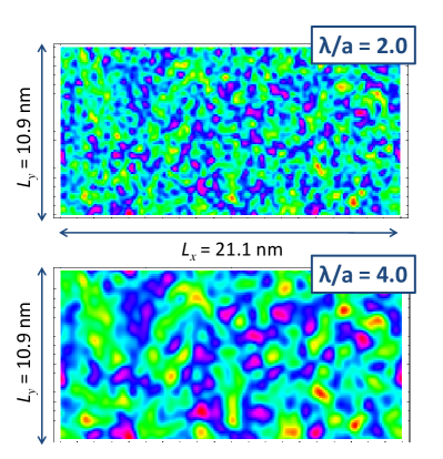
Figure 1: Typical spatial “landscapes” of the fluctuation in the hopping matrix elements $\delta t_{ij}/W=(t_{ij}-t)/W$ for two different correlation lengths ($\lambda=2a,4a$). The color scale represents the magnitude of $\delta t_{ij}/W$. The lattices shown above have $M$$\times$$N$ = 100$\times$90 atoms, which corresponds to lateral dimensions $L_{x}$$\times$$L_{y}$ = 21.1 nm $\times$ 10.9 nm.

We consider graphene lattices of $M$$\times$$N$ carbon atoms ($M$ zigzag chains, each containing $N$ atoms) with periodic boundary conditions. The linear sizes of the lattices are

$$L_{x}=(M-1)\frac{\sqrt{3}}{2}a,\;\;\;\;\,\,\,\,\,L_{y}=(N-1)\frac{a}{2}.$$ (2)

Most of the numerical results shown in this paper are calculated for lattices of $M$$\times$$N$ = 100$\times$90 atoms, corresponding to a size $L_{x}$$\times$$L_{y}$ = 21.1 nm $\times$ 10.9 nm, the same lattice dimensions shown in Fig. 1.

III Dirac Hamiltonian: analytical results

Near half filling, the low-energy properties of the tight-binding Hamiltonian in Eq. (1) are described by noninteracting massless Dirac fermions in an uniform perpendicular magnetic field, with an effective Hamiltonian given by Shon and Ando (1998); Zheng and Ando (2002)

$$H_{0}=v_{F}\begin{pmatrix}0&\pi_{x}-i\pi_{y}&0&0\\ \pi_{x}+i\pi_{y}&0&0&0\\ 0&0&0&\pi_{x}+i\pi_{y}\\ 0&0&\pi_{x}-i\pi_{y}&0\end{pmatrix},$$ (3)

where $\hbar v_{F}=\sqrt{3}at/2$ is the Fermi velocity, $\bm{\pi}=\bm{p}+e\bm{A}/c$, and $\bm{p}$ stands for the electron momentum operator. The Hamiltonian (3) operates on a four-components wave function $(\Psi^{K}_{A},\Psi^{K}_{B},\Psi^{K^{\prime}}_{A},\Psi^{K^{\prime}}_{B})$, where $\Psi^{K}_{A}$ and $\Psi^{K}_{B}$ represent the envelope functions at $A$ and $B$ sites for the $K$ point and $\Psi^{K^{\prime}}_{A}$ and $\Psi^{K^{\prime}}_{B}$ for $K^{\prime}$, respectively. In this paper we do not consider explicitly the electron spin degree of freedom and all states are assumed spin degenerate.

The eigenstates of the Hamiltonian (3) are labeled by $(j,n,k)$, with the valley index $j=K,K^{\prime}$, the Landau level index $n=0,\pm 1,\dots$, and the wave vector $k$ along $y$ direction.Shon and Ando (1998) The eigenenergy depends solely on $n$ as $\varepsilon_{n}=\hbar\omega_{B}\,\,{\rm sgn}(n)\sqrt{|n|}$, where $\hbar\omega_{B}=\sqrt{2}\gamma/\ell_{B}$ with the magnetic length given by $\ell_{B}=\sqrt{\hbar/eB}$. For $\Phi/\Phi_{0}<0.05$, which implies $\ell_{B}/a\gg 1$, lattice size effects have a negligible influence on the graphene LLs in this model.

The eigenfunctions are written as

$$\Psi^{K}_{nk} = \frac{C_{n}}{\sqrt{L}}\exp(iky)\left(\begin{array}[]{c}{\rm sgn}(n)(-i)\phi_{|n|-1,k}\\ \phi_{|n|,k}\\ 0\\ 0\end{array}\right),$$ (8)

$$\Psi^{K^{\prime}}_{nk} = \frac{C_{n}}{\sqrt{L}}\exp(iky)\left(\begin{array}[]{c}0\\ 0\\ \phi_{|n|,k}\\ {\rm sgn}(n)(-i)\phi_{|n|-1,k}\end{array}\right).$$ (13)

Here $C_{n}=1$ for $n=0$, $C_{n}=1/\sqrt{2}$ for $n\neq 0$, and

$$\phi_{n,k}(x)=(2^{n}n!\sqrt{\pi}\ell_{B})^{-1/2}\,\,e^{-z^{2}/2}H_{n}(z),$$ (14)

with $z=(x-k\ell_{B}^{2})/\ell_{B}$ and $H_{n}(z)$ denoting Hermite polynomials.

It was realized early Koshino and Ando (2007) that the level with $n=0$ is special since its amplitude is non-zero only in one of the sublattices, namely, at $B$ sites for $K$ and $A$ sites for $K^{\prime}$. Consequently, while a random on-site disorder potential gives only intravalley mixing within either the $K$ and $K^{\prime}$ valleys, random hopping causes intervalley mixing. (Notice that this is quite the opposite of what occurs at zero magnetic field when diagonal disorder is present.) The wave function in LLs with $n\neq 0$ has nonzero amplitudes on both $A$ and $B$ sites, so that intervalley mixing is always possible.

In this study, we consider hopping disorder caused by randomness in the hopping integral connecting neighboring $A$ and $B$ sites. This disorder can be long ranged, when caused by static ripples, or short ranged, when originated by scatterers located at points in-between neighboring sites.

Assuming that $t$ shifts to $t+\delta t$ between neighboring sites ${\bm{R}}_{A}$ and ${\bm{R}}_{B}$, hopping disorder gives rise to a short-range potential given byKoshino and Ando (2007)

$$U({\bm{r}})=\left(\begin{array}[]{cccc}0&z_{A}^{*}z_{B}&0&z_{A}^{*}z_{B}^{\prime}\\ z_{B}^{*}z_{A}&0&z_{B}^{*}z_{A}^{\prime}&0\\ 0&z_{A}^{\prime*}z_{B}&0&z_{A}^{\prime*}z_{B}^{\prime}\\ z_{B}^{\prime*}z_{A}&0&{z_{B}^{\prime}}^{*}z_{A}^{\prime}&0\end{array}\right)u_{\rm h}\delta({\bf r}-{\bf R}_{i}),$$ (15)

with $u_{\rm h}=(\sqrt{3}a^{2}/2)\delta t$, $z_{X}=e^{i{\bf K}\cdot{\bf R}_{X}}$, and $z^{\prime}_{X}=e^{i{\bf K}^{\prime}\cdot{\bf R}_{X}}$ for $X=A$ and $B$. For a hopping disorder concentration $n_{\rm h}$, the self-consistent Born approximation estimates the Landau level broadening as $\Gamma_{\rm short}=(2n_{\rm h})^{1/2}u_{\rm h}/(\pi\ell_{B})$, independent of Landau level index. Numerical simulations Pereira (2009) exhibit the same scaling of $\Gamma_{\rm short}$ with $\sqrt{B}$, but show that $\Gamma_{\rm short}$ increases with the index $n$.

Alternatively, when the randomness in the hopping integrals shows long-range correlations, the disorder Hamiltonian can be formulated in terms of an effective random magnetic field.Abanin et al. (2007); Vozmediano et al. (2010) In this case, one assumes that lattice deformations cause a smooth shift in the hopping integrals between the site $j$ and its three nearest neighbors $i$. At low energies, this effect can be incorporated into Dirac Hamiltonian by introducing an effective vector potential that reads

$$A^{\rm eff}_{\pm}({\bm{r}}_{j})=\frac{c}{e}\sum_{i=1}^{3}\delta t_{i}({\bm{r}}_{j})e^{\pm i{\bm{q}}_{0}\cdot\hat{{\bm{e}}}_{i}}.$$ (16)

Here, $A^{\rm eff}_{\pm}=A^{\rm eff}_{x}\mp iA^{\rm eff}_{y}$, ${\bm{e}}_{i}$ are vector connecting a lattice site to its neighbors, and ${\bm{q}}\approx\pm{\bm{q}}_{0}$, where ${\bm{q}}_{0}=4\pi/(3\sqrt{3}a){\bm{e}}_{y}$ with the Cartesian coordinate $x$ running along the armchair direction. The subscript $+\ (-)$ corresponds to the $K\ (K^{\prime})$ valley. Random hopping is accounted for by adding the effective vector potential ${\bm{A}}^{\rm eff}$ to the momentum operator $\bm{\pi}$ appearing in Eq. (3), namely,Abanin et al. (2007)

$$H_{\pm}=v_{F}\begin{pmatrix}0&\pi_{x}-i\pi_{y}+\frac{e}{c}A_{\pm}^{\rm eff}\\ \pi_{x}+i\pi_{y}+\frac{e}{c}A_{\pm}^{\rm eff*}&0\end{pmatrix}.$$ (17)

Notice that the effect of $A^{\rm eff}_{\pm}$ is to locally shift the Dirac cones $K$ and $K^{\prime}$ in opposite directions and there is no valley mixing. The structure of $H_{\pm}$ immediately reveals that the $n=0$ states are unique: Since $\langle\Psi^{K}_{0k}|H-H_{0}|\Psi^{K^{\prime}}_{0k^{\prime}}\rangle=0$, in lowest order, long-range hopping disorder does not affect the $n=0$ states.

Unfortunately, there is no such simple picture for treating the crossover regime between short- and long-range hopping disorder. In the following, we interpret the results of our numerical simulations by invoking the pure long-range description provided by Eq. (17), what is known about short-range hopping disorder, and by building a plausible interpolation between these two limits.

IV Spectral properties

In this Section, we analyze the spectral properties of graphene obtained from the tight-binding model with correlated random hopping presented in Sec. II. We will focus our attention on the width of the disorder-broadened Landau levels and its dependence on the disorder correlation length $\lambda$, on the disorder amplitude $W$, on the magnetic flux $\Phi$, and on the LL index $n$.

Figure 2a shows the density of states (DOS) corresponding to the four lowest LLs ($n=0,1,2$, and $3$) broadened by a correlated random hopping disorder of amplitude $W/t=0.3$ for different correlation lengths, namely, $\lambda/a$ = 1, 2, and 4. Since particle-hole symmetry is preserved by the nearest-neighbor hopping disorder model, we only show the $n\geq 0$ LLs. The magnetic flux considered is $\Phi/\Phi_{0}$=0.02. The results typically correspond to averages over 600 disorder realizations.

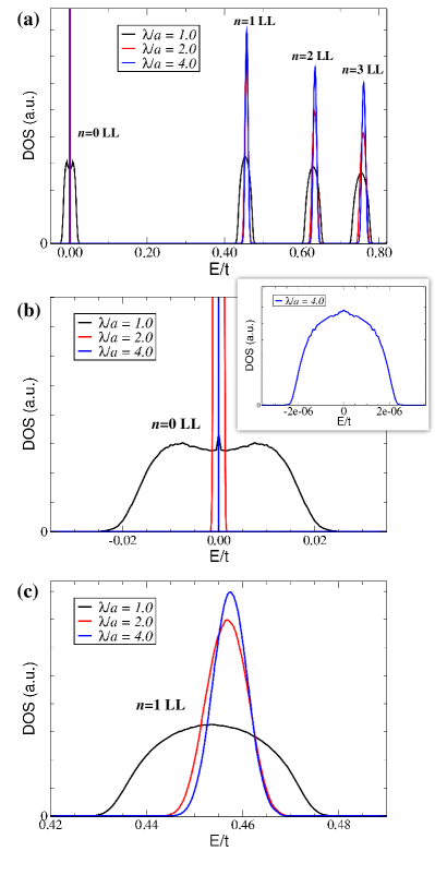
Figure 2: Density of states (in arbitrary units) for a magnetic flux $\Phi/\Phi_{0}$=$0.02$ for three different correlation lengths $\lambda/a$ of the random hopping potential (in all cases $W/t=0.3$ and the lattice size is $M$$\times$$N$=100$\times$90 sites). (a) DOS showing the $n$=0, 1, 2, and 3 Landau bands. (b) Zoom of the $n=0$ LL states. (c) Zoom of the $n=1$ LL states.

Figures 2b and 2c are zooms of the DOS around the $n$=0 and the $n$=1 LLs, respectively, indicating that the broadening shrinks for increasing values of $\lambda$. An inspection of Fig. 2c shows that, for the $n=1$ LL, an increase in the correlation length causes only small modifications on the shape of this Landau band, plus an overall reduction of the width $\Gamma_{1}$. Higher Landau levels, $n>1$, show the same qualitative behavior as $n=1$. In contrast, for the $n$=0 LL (Fig. 2b), one observes a much stronger suppression of the level broadening upon increasing $\lambda$, in agreement with numerical results obtained in Ref. Kawarabayashi et al., 2009. However, the inset of Fig. 2b shows that, despite the large reduction of $\Gamma_{0}$ with increasing $\lambda$, the width never goes to zero within the range of $\lambda$ we used. This is at odds with the results reported in Ref. Kawarabayashi et al., 2009, where an abrupt transition to zero width was observed. It is worth mentioning that, when $\lambda$ increases, making the width of the $n=0$ LL much smaller than the width of the higher levels, it is important to use DOS histograms with a much finer energy resolution around the $n=0$ LL than for the higher LLs. Not doing so can lead to an erroneous impression that the $n=$ LL width vanishes sharply as the correlation length increases.

In the following, we describe how we define and quantify the width $\Gamma_{n}$ of the disordered-broadened LLs. For the $n>0$ LLs, which display a Gaussian-like shape, $\Gamma_{n}$ is taken as the full width at half-height. Figure 2 clearly shows that the DOS shape of the $n=0$ LL is very different from the higher LLs. As pointed out in Ref. Pereira, 2009, an off-diagonal disorder model induces a splitting of the $n=0$ LL into two degeneracy-broken $n=0$ Landau bands, causing the observed DOS shape for the $n=0$ LL, namely, not fully split levels. This is so because the energy splitting always has the same order of magnitude of the LL broadening. Here, the $n=0$ LL shapes observed in Fig. 2b can be reasonably well fitted by a superposition of two equal Gaussian curves. Therefore, the $n=0$ LL width is considered as the width at half-height of one of these superposed bands (which is approximately half the width at half-height of the entire band).

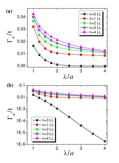
Figure 3: Width of the $n$th Landau level $\Gamma_{n}/t$, $n=0,1,2,3,4$, as a function of the disorder correlation length $\lambda/a$ for $\Phi/\Phi_{0}=0.02$ and $W/t=0.3$. (a) Linear scale. (b) Log-linear scale.

Figure 3 shows how the LL widths decrease as the hopping disorder correlation length grows. In Fig. 3a, one observes that not only $\Gamma_{0}$ decreases with $\lambda$, but all other LLs do so. When examining the same data in a log-linear graph (Fig. 3b), one observes that the $n=0$ LL behaves quite differently from the others. For $n>0$, the widths $\Gamma_{n}$ decrease slowly with increasing $\lambda/a$. Figure 3 shows an apparent tendency to saturation at a value $\Gamma_{n}/t\approx 0.01$. We computed $\Gamma_{n>0}$ for larger values of $\lambda/a$ (not shown here) and concluded that this in not quite correct. Instead, we observe that the rate by which all $\Gamma_{n>0}$ decrease becomes smaller as $\lambda/a$ becomes larger. The behavior is very different for the $n$=0 LL, whose width decays exponentially with $\lambda$. This decay is sustained down to the numerical precision of our simulations.

Further insight about the effect of long-range correlated hopping disorder on the levels widths $\Gamma_{n}$ can be gained from a perturbation theory analysis. Let us denote the disorder gauge potential by $V=H_{\pm}-H_{0}$, where both $H$ and $H_{0}$ are defined in Sec. III.

In first order, the matrix elements required to calculate the energy corrections for the degenerate states that belong to the $n$th Landau level at the $K$ valley are

$$V_{nK,kk^{\prime}}^{(1)}=\langle\Psi_{n^{\prime}k^{\prime}}^{K}|V|\Psi_{nk}^{K}\rangle.$$ (18)

Since long-range hopping disorder does not mix valleys, $K$ is a good quantum number in this model. As discussed in Sec. II, $E_{0}^{(1)}=0$. For $n>0$, the situation is different. Exact diagonalization in a $(n>0,K)$ subspace involves matrix elements of the kind $V_{n\neq 0,K;kk^{\prime}}^{(1)}$. Due to the spinor structure of $\Psi_{nk}^{K}$, the evaluation of such matrix elements amounts to the spatial integration of the product $\exp[i(k-k^{\prime})y]\phi_{nk^{\prime}}(x)\phi_{n-1,k}(x)$ times the Gaussian fluctuating gauge potential. This results in non-zero matrix elements, but they are very quickly suppressed as $\lambda/\ell_{B}$ becomes large.

Let us define

$$V_{nK,kk^{\prime}}^{(2)}={\sum_{n^{\prime}\neq n}}\frac{|\langle\Psi_{n^{\prime}k^{\prime}}^{K}|V|\Psi_{nk}^{K}\rangle|^{2}}{\hbar\omega_{B}(\sqrt{n^{\prime}}-\sqrt{n})}$$ (19)

to help us to discuss second-order effects. The evaluation of $V_{n=0,K;kk^{\prime}}^{(2)}$ involves matrix elements where products of $\phi_{1,k^{\prime}}$ and $\phi_{0,k}$ appear. For long-range disorder, such matrix elements vanish with increasing $\lambda/\ell_{B}$. In summary, the perturbation fails to mix states within the $n=0$ multiplet and also with $n^{\prime}\neq 0$. Hence, we expect the same behavior at all order of perturbation theory. This is consistent with statement that $\Gamma_{0}=0$ for long-range hopping disorder.Ostrovsky et al. (2008) Using the reasoning presented above, matrix elements of the kind $V_{n\neq 0,K;kk^{\prime}}^{(2)}$ involve, among other components, the integration of products wave function amplitudes such as $\exp[i(k-k^{\prime})y]\phi_{nk^{\prime}}(x)\phi_{n,k}(x)$. These become small for $k\neq k^{\prime}$ in the limit of $\lambda/\ell_{B}\gg 1$ and, for $k=k^{\prime}$, are quite independent of $\lambda/\ell_{B}\gg 1$.

This analysis rules out long-range hopping disorder as the mechanism behind the exponential suppression of $\Gamma_{0}$ with increasing $\lambda$. We speculate that this behavior is caused by matrix elements that admix valleys, a remnant of the crossover regime. As a consequence, we expect $\Gamma_{0}$ to scale linearly with the disorder strength $W$ and the eigenstates to be a superposition of a wave functions with probability amplitudes in both sublattices. Our simulations are in line with the latter statement, as we discuss below.

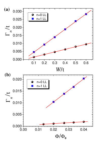
Figure 4: (a) Landau level width $\Gamma_{n}/t$ as a function of the hopping disorder strength $W/t$ for the n=0 and n=1 LLs (magnetic flux fixed at $\Phi/\Phi_{0}$=$0.02$ and $\lambda/a$=$1.5$). (b) $\Gamma_{n}$ as a function of magnetic flux $\Phi/\Phi_{0}$ for the same LLs (now for a fixed disorder strength $W/t$=$0.3$ and $\lambda/a$=$2.0$).

When a magnetic field is present, there is an important length scale to be considered, namely, the magnetic length; for convenience, let us write it in the form $\ell_{B}/a$=0.371$/\sqrt{\Phi/\Phi_{0}}$. For the magnetic flux used in our simulations ($\Phi/\Phi_{0}$=$0.02$), we obtain $\ell_{B}/a$=$2.62$, which is close to the values of $\lambda/a$ used as well. Therefore, we expect the magnetic length to play a role in any interpretation of our results. Indeed, Fig. 3a suggests that the LL widths change its dependence with $\lambda$ for $\lambda\gtrsim\ell_{B}$. However, Fig. 3b makes clear that a slow dependence on $\lambda$ only occurs for the $n>$0 LL. This is in line with our perturbative analysis. Unfortunately, the picture is not entirely consistent: We expect the second-order terms to be dominant in the calculation of the broadening of $\Gamma_{n>0}$ for $\lambda/\ell_{B}$, which is not observed in the simulations (see discussion below). This remains to be understood.

We call attention to the fact that the authors of Ref. Kawarabayashi et al., 2009 used the same flux value we considered here, as well as a similar range for the correlation length $\lambda$. However, in our calculations, a finite width of the $n=0$ LL can be seen even for $\lambda/a$=$4$ within the numerical precision we use. We checked (not shown here) that these results are not influenced by varying the system sizes, i.e, there are no finite lattice-size effects in the parameter region we investigated.

We have also investigated the dependence of the $n=0$ and $n=1$ LLs widths on the disorder and magnetic field amplitudes (Fig. 4). For both parameters, there is a clear linear increase.

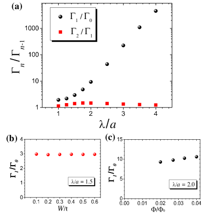
Figure 5: (a) Ratio between different Landau level widths $\Gamma_{n}/\Gamma_{n-1}$ as a function of $\lambda/a$. The ratio between higher LLs widths, like $\Gamma_{2}/\Gamma_{1}$, is quite independent of the correlation length $\lambda$. In contrast, the ratio $\Gamma_{1}/\Gamma_{0}$ grows rapidly with $\lambda/a$ (notice the logarithmic scale). (b) Ratio $\Gamma_{1}/\Gamma_{0}$ as a function of the disorder strength $W/t$ for $\lambda/a=1.5$. (c) Ratio $\Gamma_{1}/\Gamma_{0}$ as a function of the magnetic flux $\Phi/\Phi_{0}$ for $\lambda/a=2.0$. The panels (b) and (c) show that $\Gamma_{1}/\Gamma_{0}$ is almost independent of $W/t$ and $\Phi/\Phi_{0}$. In the log-linear plot of panel (a) the results corresponding to different values of $W/t$ and $\Phi/\Phi_{0}$ collapse under the same dot.

Since the LL widths depend linearly on $W$ and on $\Phi/\Phi_{0}$, we conclude that there is universality in the behavior of the Landau level widths, namely, the ratio between different Landau level widths, $\Gamma_{n}/\Gamma_{n^{\prime}}$, depends solely on $\lambda/a$. This is illustrated in Fig. 5a, where one can see the ratio $\Gamma_{1}/\Gamma_{0}$ growing rapidly with $\lambda/a$ (notice the logarithmic scale), while $\Gamma_{2}/\Gamma_{1}$ remains essentially constant. This novel result allows our simulations to make contact with the experiments. Notice that due to computational limitations, our lattices sizes constrain us to consider unrealistically large values of magnetic field magnitudes. However, since the ratios of LL widths are rather insensitive to the values of $W$ and $\Phi/\Phi_{0}$, as illustrated by Figs. 5b and c, we expect this result to apply for realistic settings as well.

The dependence of the width on the LL index is shown in Fig. 6. In this case as well, $\Gamma_{n}$ increases with $n$ when $\lambda$, $W$, and $\Phi$ are fixed (notice that the values for these parameters are the same considered in Fig. 3). We find that for $\lambda/a=2$, the $\Gamma_{n}$ versus $n$ curve is perfectly fitted by the functional form $y=A\sqrt{x}$, with $A$=0.0107 (dashed line in Fig. 6). For other values of $\lambda$, including the cases $\lambda/a=1$ and $\lambda/a=4$, the numerical data do not show a square root dependence on LL index $n$. At this point, it is worth comparing these results to the effect of a diagonal disorder on the DOS in graphene at the quantum Hall regime. The Landau level broadening $\Gamma_{n}$ for a diagonal white-noise disorder is quite independent of the LL index $n$, Pereira and Schulz (2008); Zhu et al. (2009) while for the correlated diagonal disorder, $\Gamma_{n}$ is observed to slightly decrease with increasing $n$.Pereira and Schulz (2008) These effects for the diagonal disorder in graphene are similar to the observed for conventional quantum Hall systems with diagonal disorder models,Ando and Uemura (1974) but are in clear contrast to the increase of $\Gamma_{n}$ with $n$ observed here.

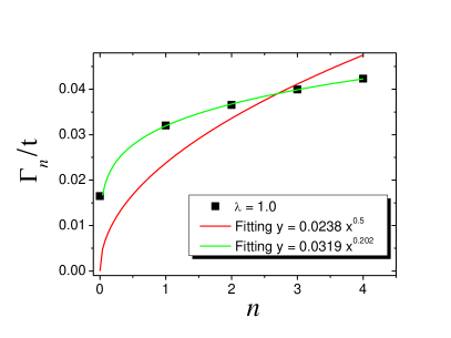
Figure 6: Landau level width $\Gamma_{n}/t$ as a function of LL index $n$ for three different values of $\lambda/a$, considering $\Phi/\Phi_{0}=0.02$ and $W/t=0.3$ (same magnetic flux, disorder amplitude, and lattice sizes considered in Fig. 3). The dashed line corresponds to a fitting with square root dependence, which fits well only the $\lambda/a=2$ case (see text).

V Localization properties

While in Sec. IV we considered the DOS and analyzed the LL widths as a function of several parameters, we now investigate the localization properties of states within the LLs. To infer the degree of localization of the states we use the participation ratio (PR), which is defined as Thouless (1974)

$${\rm PR}=\frac{1}{N^{\prime}\sum_{i=1}^{N^{\prime}}|\psi_{i}|^{4}},$$ (20)

where $\psi_{i}$ is the amplitude of the normalized wave function on site $i$ and $N^{\prime}=M\times N$ is the total number of lattice sites. The PR is therefore directly related to the proportion of the lattice sites over which the wave function is spread: the PR for a localized state vanishes in the thermodynamic limit, while peaks in the PR indicate the presence of extended states (critical energies).

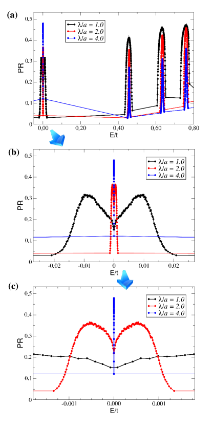
Figure 7: Participation Ratio as a function of $E/t$ for different random hopping correlation lengths $\lambda/a$. Here ,$\Phi/\Phi_{0}=0.02$, $W/t=0.3$, and $M$$\times$$N$=100$\times$90 (namely, the same magnetic flux, disorder amplitude, and lattice sizes considered in Fig. 3). (a) Energy window containing the four lowest LLs, $n$=0, 1, 2, and 3. (b) Zoom on the $n=0$ Landau level. (c) Amplified zoom on the $n=0$ states.

Figure 7a shows the calculated PR in an energy window comprising the Landau levels $n$=0, 1, 2, and 3. While the PR for the $n>0$ LLs indicates the presence of localized states at Landau band tails and extended states at the band middle, as expected, the PR of the states from the $n=0$ LL shows a double hump structure, i.e., a splitting into two peaks. The splitting is more clearly observed in the energy scale zooms of Fig. 7b and c. This splitting of critical energies in the lowest LL was previously observed and discussed for uncorrelated random hopping disorder Koshino and Ando (2007); Pereira (2009) (and for the similar case of uncorrelated random magnetic flux disorder Schweitzer and Markoš (2008); Schweitzer (2009)). The novel and interesting aspect we observe here is that the splitting is rather robust and survives even the sharp width reduction of the $n$=0 LL due to the increasing correlation length. While previous works considered correlated random hopping disorder, Kawarabayashi et al. (2009, 2010) they did not calculate the localization properties of the states within LLs and therefore missed this splitting of critical states at $n=0$.

Although experiments Jiang et al. (2007b) have observed this splitting energy in the $n$=0 LL, it is hard to make a quantitative comparison due to the lattice size compromises we need to make in our simulations. Moreover, we believe that a full explanation of the experimentally observed splitting requires taking into account the Zeeman term and possibly electron-electron interactions, which calls for further theoretical investigation.

Due to particle-hole symmetry, the probability densities $|\Psi(E)|^{2}$ and the PR of states at energies $-E$ and $+E$ are identical (see, for instance, Ref. Abergel et al., 2010 and references therein). However, when looking directly at the wave function amplitudes $\Psi(E)$, one can see a difference between the split states at $-E$ and $+E$: In one of the sublattices (sublattice $A$, for example) the amplitudes are exactly the same, while in the other sublattice ($B$) they have the same magnitude but opposite signs, that is, $\Psi_{A}(-E)=\Psi_{A}(+E)$ and $\Psi_{B}(-E)=-\Psi_{B}(+E)$. This guarantees that conjugated particle-hole states are orthogonal and have the same probability densities $|\Psi(E)|^{2}$. It is noteworthy that orthogonality imposes that the probability weight at both sublattices is the same. The split states are therefore similar to bonding-antibonding states. The table in Fig. 8 summarizes these features.

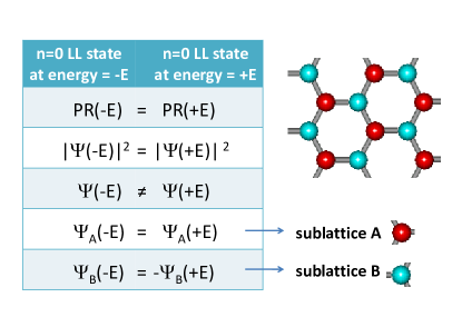
Figure 8: Properties of the wave functions $\Psi$ for $n=0$ LL states at energies $+E$ and $-E$. While the PR and the probability densities of the wave functions $|\Psi(E)|^{2}$ are identical for states at energies $-E$ and $+E$, the wave function amplitudes $\Psi(E)$ show differences in only one of the sublattices, in analogy to bonding-antibonding states (see text).

Another feature observed in Fig. 7 is the effect of increasing correlation length. The effect on the $n$=0 LL is completely different (opposite) to what is observed in higher levels. In higher levels, the increase in $\lambda$ causes an overall reduction of PR values, while in the $n$=0 LL, despite the suppression of broadening (see Sec. IV), one observes an overall increase in the PR. This difference in behavior is probably related to the fact that the states from the higher levels have much longer localization lengths than those from the states with $n$=0. Ando and Uemura (1974) To investigate possible finite-size effects on the $n=0$ LL when $\lambda/a$ is large, we ran simulations with larger lattice sizes (not shown). We found no change in the position of the identified critical states, as well as no change in the LL widths.

VI Conclusions

We have investigated the effects of spatially correlated random hopping disorder on the structure of Landau levels in graphene. We quantified the behavior of the $n$th Landau level width $\Gamma_{n}$ as a function of the correlation length, as well as other relevant parameters of the system: disorder amplitude, magnetic field, and Landau level index $n$. We found that $\Gamma_{n}$ gets narrower with increasing correlation length for all Landau levels, and not only for the $n=0$ level. However, a logarithmic plot of $\Gamma_{n}$ as function of $\lambda$ (Fig. 3b) clearly showed that while for $n>0$ the widths decrease slowly, for $n=0$ they decay exponentially with increasing $\lambda$. We found no sign of any abrupt vanishing of the $n=0$ Landau level width at finite $\lambda$. This suggests that a different physical mechanism is behind the narrowing of the $n=0$ LL when compared to all the other levels (specially when the correlation length $\lambda$ becomes of the same order of magnitude or higher than the magnetic length $\ell_{B}$). We speculate that the underlying mechanism is due to valley mixing, remnant of the crossover regime.

$\Gamma_{n}$ increases linearly with both magnetic field and disorder amplitude. Another interesting observation is that for any fixed correlation length, $\Gamma_{n}$ always increases with increasing LL index $n$, which is completely different to the dependence observed for diagonal (on-site) disorder models. More importantly, we observe that the ratio between the n=1 and n=0 Landau level widths, $\Gamma_{1}/\Gamma_{0}$, depends only on the correlation length $\lambda$ and is rather insensitive to the disorder strength and to the magnitude of the applied magnetic field. This allows a closer contact of our results with experiments. In Ref.  Giesbers et al., 2009a, for instance, the authors experimentally observe a $n=0LL$ width of about 20K, while the width of higher levels is observed to be about 400K that is $\Gamma_{1}/\Gamma_{0}=20$. Using this information and the results of our Fig. 5, we infer that $\lambda/a=2.2$. This estimate gives a lower bound for the corrugation length of graphene in the experiment of Ref. Giesbers et al., 2009a, since it neglects all disorder broadening sources but hopping disorder.

We also considered the role played by changing the hopping disorder correlation length on the localization properties of the states within the different Landau levels. The splitting of two critical energies for the $n=0$ level, previously reported for uncorrelated random hoppings,Pereira (2009) is still clearly defined for correlated hopping disorder. It is a robust effect even with the sharp width reduction of the $n=0$ level that occurs for large values of $\lambda$. The $n=0$ level can therefore be considered as a superposition of two levels with broken degeneracy, symmetrically split around $E=0$. In addition, after analyzing the wave functions of states belonging to the $n=0$ level, we were able to identify a symmetric structure of these states. We found that although any two states at $-E$ and $+E$ have the same probability density and also the same participation ratio, in one sublattice the wave function amplitudes of states with energies $\pm E$ are exactly the same, while in the other sublattice these states have the same magnitude but opposite signs. Therefore, the origin for this $n=0$ level splitting is clearly related to the breaking of the sublattice degeneracy induced by the hopping disorder, a further manifestation of the influence of valley mixing disorder.