Scaling of ground state fidelity in the thermodynamic limit: XY model and beyond

Abstract

We study ground state fidelity defined as the overlap between two ground states of the same quantum system obtained for slightly different values of the parameters of its Hamiltonian. We focus on the thermodynamic regime of the XY model and the neighborhood of its critical points. We describe in detail cases when fidelity is dominated by the universal contribution reflecting quantum criticality of the phase transition. We show that proximity to the multicritical point leads to anomalous scaling of fidelity. We also discuss fidelity in a regime characterized by pronounced oscillations resulting from the change of either the system size or the parameters of the Hamiltonian. Moreover, we show when fidelity is dominated by non-universal contributions, study fidelity in the extended Ising model, and illustrate how our results provide additional insight into dynamics of quantum phase transitions. Special attention is put to studies of fidelity from the momentum space perspective. All our main results are obtained analytically. They are in excellent agreement with numerics.

I Introduction

Quantum phase transitions (QPTs) happen when dramatic changes in the ground state properties of a quantum system can be induced by a tiny variation of an external parameter Sachdev (1999). This system-specific parameter can be a magnetic field in spin systems Coldea et al. (2010); sad , intensity of a laser beam in cold atom simulators of Hubbard-like models Hub , dopant concentration in high-Tc superconductors Lee et al. (2006), etc.

Traditional condensed matter approaches to QPT focus on identification of the order parameter and the pattern of symmetry breaking as well as on studies of two point correlation functions and the excitation gap Sachdev (1999). At the critical point of the second order QPT the correlation length diverges while the gap in the excitation spectrum vanishes. This is typically described by power-law singularities. Correlation length $\xi$ diverges as $|\lambda-\lambda_{c}|^{-\nu}$, while the excitation gap closes as $|\lambda-\lambda_{c}|^{z\nu}$, where $\lambda$ is the external field driving the transition, $\lambda_{c}$ marks the quantum critical point, and $z$ and $\nu$ are the critical exponents associated with the universality class of the system. The exponents are universal in the sense that they do not dependent on the microscopic details of the system.

A somewhat different ways of looking at QPTs have recently emerged from quantum information community. One of them is based on studies of quantum entanglement of spins/atoms/etc. undergoing a QPT Ost . Another is based on studies of ground state fidelity Zanardi and Paunković (2006) (see Gu (2010) for a recent review). Finally, an extreme approach emerged where the Hamiltonian is designed to have a particular many-body state as its ground state Wolf et al. (2006). We will study ground state fidelity below.

More precisely, ground state fidelity, or simply fidelity, is defined here as

$${\cal F}(\lambda,\delta)=|\langle\lambda-\delta|\lambda+\delta\rangle|,$$ (1)

where $|\lambda\rangle$ is a ground state wave function of a many-body Hamiltonian $\hat{H}(\lambda)$ describing the system exposed to an external field $\lambda$, while $\delta$ is a parameter difference. It provides the most basic probe into the dramatic change of the wave function around the critical point and has the following properties

$$0\leq{\cal F}(\lambda,\delta)\leq 1,\ \ \ {\cal F}(\lambda,\delta)={\cal F}(\lambda,-\delta).$$ (2)

The recent surge in studies of fidelity follows observation that quantum criticality promotes its decay Zanardi and Paunković (2006). This is easily justified as ground states change rapidly near the critical point to reflect singularities of a QPT. Therefore, one expects that ${\cal F}(\lambda,\delta)$ has a minimum at the critical point.

The drop in fidelity encodes not only the position of the critical point, but also universal information about the transition given by the critical exponent $\nu$. This has been worked out independently in the “small system” Campos Venuti and Zanardi (2007); Schwandt et al. (2009); Albuquerque et al. (2010); Barankov (2009); De Grandi et al. (2010a, b); Pol and in the thermodynamic Rams and Damski (2011) limits. Broadly speaking the former corresponds to $\delta\to 0$ at fixed system size $N$, while the latter corresponds to $N\to\infty$ at small, fixed $\delta$.

In the “small system” limit we can Taylor expand fidelity in $\delta$ Zanardi and Paunković (2006); You et al. (2007); Gu (2010)

$${\cal F}(\lambda,\delta)\simeq 1-\delta^{2}\chi_{F}(\lambda)/2,$$ (3)

where $\chi_{F}$ stands for the so-called fidelity susceptibility. The linear term in $\delta$ disappears in the above expansion due to the normalization condition of the ground states whose overlap is taken (see e.g. Gu (2010)). This can be also seen from (2): a linear in $\delta$ term could make ${\cal F}>1$ or simply fidelity is symmetric with respect to the $\delta\to-\delta$ transformation. Universal information can be extracted from fidelity susceptibility near the critical point through the scaling: $\chi_{F}(\lambda_{c})\sim N^{2/d\nu}$, where $d$ stands for system dimensionality. Alternatively, one may look at $\chi_{F}$ away from the critical point and study $\chi_{F}(\lambda)\sim N|\lambda-\lambda_{c}|^{d\nu-2}$. More generally, the scaling of fidelity susceptibility is linked to the scaling dimension of the most relevant perturbation Campos Venuti and Zanardi (2007).

In the thermodynamic limit one obtains Rams and Damski (2011):

$$\ln{\cal F}(\lambda,\delta)\simeq-N|\delta|^{d\nu}A\left(\frac{\lambda-\lambda_{c}}{|\delta|}\right),$$ (4)

where $A$ is a scaling function. We expect the above scaling result to hold when fidelity per lattice site ($-\ln{\cal F}/N$) is well defined in the thermodynamic limit, physics around the critical point is described by one characteristic scale of length (correlation length) given by the critical exponent $\nu$, and $d\nu<2$ so that non-universal (system-specific) corrections to (4) are subleading De Grandi et al. (2010a, b); Pol .

Expression (4) can be simplified away from the critical point when $|\delta|\ll|\lambda-\lambda_{c}|\ll 1$:

$$\ln{\cal F}(\lambda,\delta)\sim-N\delta^{2}|\lambda-\lambda_{c}|^{d\nu-2}.$$ (5)

Unlike (3), (4) is nonanalytic in $\delta$ near the critical point and the Taylor expansion of fidelity in $\delta$ is inapplicable here. This singularity arises from anomalies associated with the QPT in the thermodynamic limit. All these results have been obtained in the zero temperature limit that we adopt in this work. Even though a consistent theory of fidelity in finite temperatures is still missing, several results have already been obtained Sirker (2010); Zanardi et al. (2007); Quan and Cucchietti (2009).

This article is organized as follows. Sec. II describes theoretical approaches used to study fidelity and motivation behind this research. In Sec. III we focus on fidelity in the XY model showing numerous analytical results. Sec. IV discusses fidelity of the extended Ising model Wolf et al. (2006); Cozzini et al. (2007); Zhou and Barjaktarevič (2008). In Sec. V we illustrate some connection between fidelity and dynamics of a nonequilibrium quench. Our findings are briefly summarized in Sec. VI.

II Basics of fidelity

To start, we mention that the term fidelity is used in various contexts in quantum physics to describe the similarity between two quantum states. Therefore, it is important to remember that we use it only to refer to an overlap between two ground states of the same physical system calculated for different values of its external parameters.

One of the seminal results on fidelity was obtained by Anderson decades ago Anderson (1967). He showed on a particular model that fidelity disappears in the thermodynamic limit. Similar behavior has been later found in other models and was labeled as the Anderson orthogonality catastrophe. More importantly, orthogonality catastrophe was shown to play a role in numerous condensed matter systems (see e.g. Bettelheim et al. (2006) and references therein).

While being an equilibrium quantity, fidelity shows up in nonequilibrium dynamics of quantum systems. In particular, one encounters it in the context of nonequilibrium QPTs (see Dziarmaga (2010); Polkovnikov et al. (2011) for reviews on dynamics of QPTs). For example, the scaling of density of excited quasiparticles following a quench can be derived using it De Grandi et al. (2010a, b); Pol . Moreover, an envelope of nonequilibrium coherence oscillations in a central spin problem encodes fidelity as well Damski et al. (2011).

In the context of equilibrium QPTs, fidelity has been proposed as an efficient theoretical probe of quantum criticality (the so-called fidelity approach). To appreciate its simplicity, we compare the fidelity approach to the traditional method of studies of quantum criticality based on analysis of the asymptotic decay of the two point correlation functions. First, both approaches require the same input: the ground state wave functions. Second, they provide the same information: the location of the critical point and the universal critical exponent $\nu$. Third, the conventional approach is based on the assumption that the two point correlations between spins/atoms/etc. decay semi-exponentially away from the critical point and in a power law manner at the critical point Vojta (2003). The transition from semi-exponential to the power-law decay can be tedious to study even with the recent tensor network techniques (see e.g. Zak ). Therefore, the fidelity approach is arguably a simpler alternative at least as far as numerical calculations are concerned.

On the analytical side, compact and accurate results for fidelity are scarce. Typically, models are not exactly solvable and so analytical results are out of reach for them. In exactly solvable systems situation is far from trivial as well. Indeed, in systems like the Ising model one is left with a large product of analytically known factors that have only recently been cast into a simple expression: see Rams and Damski (2011) and Sec. III. The situation is much different in some systems where ground states can be exactly expressed through finite rank Matrix Product States: see Wolf et al. (2006); Cozzini et al. (2007); Zhou and Barjaktarevič (2008) and Sec. IV. The Hamiltonians of these systems, however, are “engineered” to have a pre-determined ground state Wolf et al. (2006). These difficulties motivate various approximate approaches.

First, powerful numerical techniques have been deployed including tensor networks Zhou et al. (2008a) and Quantum Monte Carlo Schwandt et al. (2009); Albuquerque et al. (2010) simulations. These approaches provide crucial insight into models that are not exactly solvable (e.g. Schwandt et al. (2009)), and shall be especially useful for studies of systems with unknown order parameters, critical points and critical exponents.

Second, the fidelity susceptibility approach based on the Taylor expansion (3) has been used. Simplification here comes from factoring out the parameter difference $\delta$ and focusing on fidelity susceptibility that depends on the external field only. Despite these simplifications, it is typically still a mixed analytical and numerical technique. This approach is limited to studies of fidelity between very similar ground states whose overlap is close to unity. In particular, this rules out description of Anderson orthogonality catastrophe within this framework.

Third, the fidelity per lattice site approach has been proposed Zhou and Barjaktarevič (2008); Zhou et al. (2008b, a). It is in a sense “orthogonal” to the fidelity susceptibility approach as (i) it targets overlap between any two ground states: any $\delta$ is considered; (ii) it focuses on the large system limit, i.e., the opposite of what the fidelity susceptibility approach does; and (iii) fidelity typically departs significantly from unity here. This approach has been explored mostly numerically so far.

Our studies assume two most plausible features of the above two approaches Rams and Damski (2011). First, the thermodynamic limit from the fidelity per lattice site approach which allows us to study fidelity in systems well approximating the critical (infinite) ones. Second, small $\delta$ as in fidelity susceptibility approach allowing for derivation of universal scaling results such as (4) and (5). Moreover, combination of the two assumptions allows for derivation of compact analytical results for fidelity in some exactly solvable models: the task presumably impossible otherwise.

III XY model

In this section we are going to study fidelity of the XY model

$$\hat{H}=-\sum_{n=1}^{N}\left(\frac{1+\gamma}{2}\sigma^{x}_{n}\sigma^{x}_{n+1}+\frac{1-\gamma}{2}\sigma^{y}_{n}\sigma^{y}_{n+1}+g\sigma^{z}_{n}\right),$$ (6)

where we assume periodic boundary conditions $\sigma_{N+1}=\sigma_{1}$. This model is exactly solvable via the Jordan-Wigner transformation translating it into a free fermionic system Sachdev (1999); Lieb et al. (1961); Barouch and McCoy (1971); Bunder and McKenzie (1999).

Above $g$ is the external magnetic field acting along the $z$ direction and $\gamma$ is the anisotropy of spin-spin interactions on the $xy$ plane. The critical exponent $\nu$ for Ising-like critical points, $g=\pm 1,\gamma\neq 0$ and $-1<g<1,\gamma=0$ is

$$\nu=1.$$ (7)

The specific case of a multicritical point located at $g=\pm 1$ and $\gamma=0$ needs special attention Damle and Sachdev (1996). It has been proposed that there are two divergent characteristic length scales that have to be taken into account around it: one characterized by the scaling exponent $\nu=1/2$ and the other by $\nu=1$ Mukherjee et al. (2011).

We will study here

$${\cal F}=|\langle g_{1},\gamma_{1}|g_{2},\gamma_{2}\rangle|,$$ (8)

where $|g,\gamma\rangle$ is the ground state of (6). As depicted in Fig. 1, we choose $(g_{i},\gamma_{i})$ to lie on straight lines near critical points/lines.

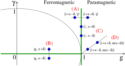
Figure 1: (Color online). Phase diagram of the XY model (6). Critical points lie on green (thick) lines. (A) to (D) show different characteristic lines along which we calculate fidelity. The dashed “circle” separates two regions of the ferromagnetic phase differing by the structure of the excitation gap. Minimum of the energy gap is reached for $k_{c}=0$ outside the “circle” ($k_{c}=\pi$ for $g<0$) and for $k_{c}=\arccos[g/(1-\gamma^{2})]$ inside the “circle” (see e.g. Bunder and McKenzie (1999)).

The analytic expression for fidelity in the XY model was given in Zanardi and Paunković (2006): ${\cal F}=\prod_{k>0}\left|\cos\left(\theta^{1}_{k}/2-\theta^{2}_{k}/2\right)\right|$, where $\tan\theta^{i}_{k}=\gamma_{i}\sin k/\left(g_{i}-\cos k\right)$ and momenta $k$ are given by (10). We have reworked it to the form which proves to be convenient for subsequent analytical studies

$${\cal F} =\prod_{k>0}f_{k},$$ (9)

$$k =(2n+1)\pi/N,\ n=0,1,\ldots,N/2-1,$$ (10)

$$f_{k} =\sqrt{\frac{1}{2}+\frac{1}{2}\frac{p_{k}}{\sqrt{p_{k}^{2}+q_{k}^{2}}}},$$ (11)

$$p_{k} =(g_{1}-\cos k)(g_{2}-\cos k)+\gamma_{1}\gamma_{2}\sin^{2}k,$$ (12)

$$q_{k} =[\gamma_{2}(g_{1}-\cos k)-\gamma_{1}(g_{2}-\cos k)]\sin k,$$ (13)

which is valid for any $g_{1}$, $g_{2}$, $\gamma_{1}$ and $\gamma_{2}$. To be more precise, we assume even $N$ and follow notation from Dziarmaga (2005) during diagonalization of (6). The ground state lays then in a subspace with even number of quasiparticles which leads to (10). In that subspace the XY Hamiltonian (6) is diagonalized to the form $\hat{H}=\sum_{k>0}\epsilon_{k}\left(\gamma_{k}^{\dagger}\gamma_{k}+\gamma_{-k}^{\dagger}\gamma_{-k}-1\right)$, where $\gamma_{k}$ are fermionic annihilation operators and the energy gap is

$$\epsilon_{k}=2\sqrt{(g-\cos k)^{2}+\gamma^{2}\sin^{2}k}.$$ (14)

In the leading order fidelity (9) can be additionally simplified by replacing the product over momentum modes by an integral

$$\ln{\cal F}~{}=~{}\sum_{k>0}\ln f_{k}~{}\simeq~{}\frac{N}{2\pi}\int_{0}^{\pi}dk\ln f_{k},$$ (15)

which is allowed in the thermodynamic limit as all the integrals that we study are convergent everywhere (even at the critical points). We note here, however, that in some cases $\ln f_{k}$ has a logarithmic singularity adding a subleading term to the transformation from summation into integration (15). This will be discussed in details in Secs. III.1 and III.2.

III.1 Across the g=1 critical line

In this paragraph we follow the path A from Fig. 1, i.e., we substitute

$$g_{1,2}=1+\epsilon\pm\delta,\ \gamma_{1}=\gamma_{2}=\gamma,\ \epsilon=c|\delta|$$ (16)

into (8) and furthermore assume that $0<\gamma\leq 1$. The relevant critical point is at $g_{c}=1$ with the critical exponent given by (7). The relevant correlation length was calculated in Barouch and McCoy (1971) and reads

$$\xi\sim\left|\frac{1}{\ln|(g-\sqrt{g^{2}-1+\gamma^{2}})/(1-\gamma)|}\right|.$$ (17)

As long as $\gamma^{2}\gg|g-1|$, it can be approximated near the critical $g_{c}=1$ by

$$\xi\sim\frac{\gamma}{|g-1|}.$$ (18)

To use this expression for the correlation length and to find the leading, universal behavior of fidelity we keep $|\delta|,|\epsilon|\ll\gamma^{2}$ in this section. We note that it implies that we stay outside of the “circle” in Fig. 1. In this region the minimum of the energy gap is reached for the smallest value of momentum $k$ (10). This condition also keeps us away from the multicritical point at $\gamma=0$ and $g=1$, which will be investigated in Secs. III.3 and III.4.

The results of this section complement our previous studies from Rams and Damski (2011) where we have considered a special case of the Ising model: $\gamma=1$. Here – besides extending our results to $\gamma\neq 1$ – we discuss the problem in momentum space, show details of our calculations and estimate errors of our approximations.

To begin the discussion, we expect the system to crossover from the “small system” limit to the thermodynamic limit when Rams and Damski (2011)

$$\min[\xi(\lambda+\delta),\xi(\lambda-\delta)]\sim L,$$ (19)

where $\lambda$ denotes a point on the $(g,\gamma)$ plane, while $\delta$ is its displacement. The latter is in general a two-component vector. Above $\xi(\lambda)$ is the correlation length in a system exposed to the external field $\lambda$ and $L$ is the linear size of the system: $L^{d}=N$. Fidelity approaches the thermodynamic limit result when

$$\min[\xi(\lambda+\delta),\xi(\lambda-\delta)]\ll L.$$

On the other hand, when

$$\min[\xi(\lambda+\delta),\xi(\lambda-\delta)]\gg L$$

the “small system” limit is reached and the behavior of fidelity is dominated by finite size effects. We use the quotation marks to highlight that we still consider $L\gg 1$ here as QPTs shall not be studied in systems made of a few spins/atoms/etc.

We notice that the correlation length in (18) has a prefactor which is linear in $\gamma$. By changing it we will illustrate the crossover (19). To that end, we fix $N$, $\delta$ and $\epsilon=-|\delta|$ ($c=-1$) so that one of the states is exactly at the critical point, i.e. ${\cal F}=\left|\langle g_{c}-2\delta,\gamma|g_{c},\gamma\rangle\right|$. The outcome of such a calculation is depicted in Fig. 2. Two distinct regimes are visible there. In the left part of the plot, where $\gamma\approx 1$, we observe $\ln{\cal F}\sim-\gamma^{-2}$. In the right part of the plot, where $\gamma\ll 1$, we find $\ln{\cal F}\sim-\gamma^{-1}$. These two regimes correspond to the “small system” limit and the thermodynamic limit, respectively.

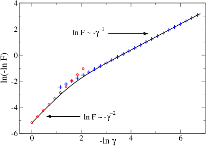
Figure 2: (Color online). Transition from the “small system” limit (left part of the plot) to the thermodynamic limit (right part of the plot) resulting from variation of the anisotropy parameter $\gamma$. Solid black line is a numerical result showing ${\cal F}=|\langle g_{c}-2\delta,\gamma|g_{c},\gamma\rangle|$, red dots depict the “small system” prediction (21), blue crosses represent the thermodynamic result (27). The figure is prepared for $\delta=3\times 10^{-7}$ and $N=10^{6}$.

Substituting (16) and (18) (with fixed $c$) into (19) we obtain the condition for the crossover as

$$\frac{N|\delta|}{\gamma}\sim 1.$$ (20)

The validity of the above condition is numerically confirmed in Fig. 3. This is done in the following way. As $-\ln\gamma$ is increased in Fig. 2, the slope of $\ln(-\ln{\cal F})$ changes smoothly from $2$ (corresponding to $\ln{\cal F}\sim-\gamma^{-2}$) to $1$ (corresponding to $\ln{\cal F}\sim-\gamma^{-1}$). The crossover region between the two limits is centered around $\gamma=\gamma_{3/2}$ where the local slope equals $3/2$. By repeating the calculation from Fig. 2 for various system sizes $N$, but the same $\delta$, we have numerically obtained $\gamma_{3/2}(N)$. A power-law fit described in Fig. 3 confirms that $\gamma_{3/2}\sim N$. Complementary analysis has been done in Rams and Damski (2011) where $\gamma=1$ and $\delta$-dependence of (20) has been verified. Based on these two calculations we conclude that the crossover condition (20) holds near the Ising critical point. In fact, it is in an excellent agreement with our numerical simulations.

After describing the crossover between the two regimes observed in Fig. 2, we can explain in detail the scaling observed on both “ends” of the plot. We start with the “small system” limit. A simple analytical calculation based on the expansion (3) – i.e. the fidelity susceptibility approach – shows that near the critical point

$${\cal F}\simeq 1-\frac{\delta^{2}N^{2}}{16\gamma^{2}}\Rightarrow\ln{\cal F}\sim\gamma^{-2}$$ (21)

because fidelity is very close to unity here. As illustrated in Fig. 2, this result agrees well with numerics. For completeness, we mention that away from the critical point, $|\epsilon|\gg|\delta|$, expansion (3) yields

$${\cal F}\simeq 1-\frac{\delta^{2}N}{16\gamma|\epsilon|},$$ (22)

in the leading order in $|\epsilon|\ll\gamma^{2}$.

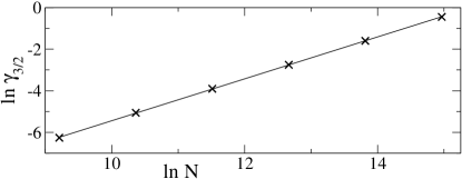
Figure 3: Numerical study of the crossover condition (20): see text for details. Crosses come from numerics, while straight line is a linear fit: $\ln\gamma_{3/2}=-15.51\pm 0.05+(1.007\pm 0.004)\ln N$ Fit . The fit shows that the crossover takes place when $\gamma\sim N$ as predicted by (20). We used here $\delta=3\times 10^{-7}$ as in Fig. 2 and extracted $\gamma_{3/2}$ from ${\cal F}=|\langle g_{c}-2\delta,\gamma|g_{c},\gamma\rangle|$.

Explanation of the thermodynamic limit result requires more involved calculations. Substituting (16) into (12-13) we obtain

$$p_{k} = (1+\epsilon-\cos k)^{2}-\delta^{2}+\gamma^{2}\sin^{2}k,$$ (23)

$$q_{k} = 2\delta\gamma\sin k.$$ (24)

To calculate $\ln{\cal F}=\ln|\langle g_{c}+\epsilon+\delta,\gamma|g_{c}+\epsilon-\delta,\gamma\rangle|$ in the leading universal order in $\delta$ we notice that the integral (15) is dominated by the contribution from small momenta $k$. This allows us to approximate (23,24) by $p_{k}\approx k^{2}\gamma^{2}+\epsilon^{2}-\delta^{2}$ and $q_{k}\approx 2\delta\gamma k$. Thus, we get

$$\ln f_{k}\approx\frac{1}{2}\ln\left(\frac{1}{2}+\frac{k^{2}\gamma^{2}+\epsilon^{2}-\delta^{2}}{2\sqrt{(k^{2}\gamma^{2}+\epsilon^{2}-\delta^{2})^{2}+(2\delta\gamma k)^{2}}}\right).$$ (25)

Next we put (25) into (15), change the integration variable $k$ there to $l~{}|\delta|/\gamma$, and send the new upper integration limit, $\pi\gamma/|\delta|$, to $\infty$. After all these approximations we obtain

$$\ln{\cal F}\simeq\frac{N|\delta|}{4\pi\gamma}\int_{0}^{\infty}dl\ln\left(\frac{1}{2}+\frac{l^{2}+c^{2}-1}{2\sqrt{(l^{2}+c^{2}-1)^{2}+4l^{2}}}\right).$$ (26)

The above integral can be calculated analytically,

$$\frac{\ln{\cal F}}{N}\simeq-|\delta|A(c)/\gamma,$$ (27)

where the scaling function

$$A(c)=\left\{\begin{array}[]{cc}\begin{split}&\frac{1}{4}+\frac{|c|K(c_{1})}{2\pi}+\frac{(|c|-1){\rm Im}E(c_{2})}{4\pi}&{\rm for}~{}|c|<1,\\ &\frac{|c|}{4}-\frac{|c|K(c_{1})}{2\pi}-\frac{(|c|-1){\rm Im}E(c_{2})}{4\pi}&{\rm for}~{}|c|\geq 1,\end{split}\end{array}\right.$$ (28)

and

$$c_{1}=-4|c|/(|c|-1)^{2},\ \ c_{2}=(|c|+1)^{2}/(|c|-1)^{2}.$$ (29)

The complete elliptic integrals of the first and second kind are defined as

$$K(x)=\int_{0}^{\pi/2}\frac{d\phi}{\sqrt{1-x\sin^{2}\phi}},E(x)=\int_{0}^{\pi/2}d\phi\sqrt{1-x\sin^{2}\phi},$$ (30)

respectively. This result is quite interesting.

First, solution (27) compares well to numerics, which is illustrated in Fig. 2 for $c=-1$. Not only the relation $\ln{\cal F}\sim-\gamma^{-1}$ is reproduced, but the whole expression fits numerics well. We mention in passing that the same good agreement was obtained for $\gamma=1$ and different $\delta$’s in Rams and Damski (2011), which confirmed the general scaling prediction (4). Notice that not the anisotropy $\gamma$ but the shift in the magnetic field $\delta$ is the relevant perturbation here.

Second, a singularity of derivative of fidelity can be obtained from (27): $\frac{d}{dc}\ln{\cal F}|_{c\to 1^{\pm}}$ is logarithmically divergent (see Rams and Damski (2011) for $\gamma=1$ case). To make a more transparent connection to the former studies of Zhou and collaborators who called such singularities as the pinch points Zhou and Barjaktarevič (2008); Zhou et al. (2008a, b), we consider $\frac{\partial}{\partial g_{2}}\tilde{d}(g_{1},g_{2})$, where the scaling parameter is defined as

$$\tilde{d}(g_{1},g_{2})=-\lim_{N\rightarrow\infty}\frac{\ln{\cal F}}{N}.$$ (31)

This can be analytically calculated from (27) to be

$$\frac{\partial}{\partial g_{2}}\tilde{d}(g_{1},g_{2})=\left.\frac{dA}{dc}\right|_{c=\epsilon/\delta}\frac{\epsilon+\delta}{2\delta\gamma}-\frac{1}{2\gamma}A\left(\frac{\epsilon}{\delta}\right),$$ (32)

where the relations between $g_{1,2}$, $\varepsilon$ and $\delta$ are specified in (16). Above we assume $g_{1}>g_{2}$ i.e. $\delta>0$. The explicit expression for (32) is quite involved and so we do not show it. It predicts a logarithmic singularity when $g_{2}\rightarrow 1$ with prefactors which depend on $g_{1}\neq 1$. More precisely, this singularity arises in the limit of $N\to\infty$, already assumed in (32), and is rounded off for finite systems: see Fig. 4. As will be shown below, it has an interesting interpretation in momentum space.

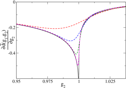
Figure 4: (Color online). Derivative of the scaling parameter: $\frac{\partial}{\partial g_{2}}\tilde{d}(g_{1},g_{2})$. Solid black line is the analytical result (32). Dashed lines from top to bottom correspond to numerical results for $N=100,300,1000,3000$, respectively. The field $g_{1}=1.1$ and $\gamma=1$.

Third, solution (27) can be simplified away from the critical point. Straightforward expansion done for $|c|\gg 1$ (but still $|\epsilon|=|c\delta|\ll\gamma^{2}$), gives $A(c)\simeq 1/16|c|$ and so

$${\cal F}~{}\simeq~{}\exp(-N\delta^{2}/16\gamma|\epsilon|)$$

in agreement with (5). When the argument of the exponent is not small, this is a new result. Otherwise, it coincides with expression (22), from the fidelity susceptibility approach (3).

Complementary insight into fidelity can be obtained in momentum space where we focus on $f_{k}$. It is presented in Fig. 5 where we show prototypical behavior of $f_{k}$ for the Ising model when: (i) the ground states entering fidelity are calculated on the opposite sides of the critical point $|c|<1$; (ii) one of them is obtained at the critical point $|c|=1$; (iii) they are both obtained on the same side of the critical point $|c|>1$.

As illustrated in Fig. 5, if $\Delta k=2\pi/N\gg|\delta|/\gamma$ only $f_{k}\approx 1$ contribute to fidelity, and we end up in the “small system” limit. The system is too small to monitor changes of $f_{k}$ between zero and unity. Still, we are able to observe universal finite size effects Schwandt et al. (2009); Albuquerque et al. (2010); Barankov (2009); De Grandi et al. (2010a, b); Pol in (21).

In the opposite limit of $\Delta k\ll|\delta|/\gamma$, we are able to approach the exact ($N\rightarrow\infty$) thermodynamic limit and the product (9) is well approximated by the integral (15) [but see the discussion below as well]. Now momenta $k$ are dense enough to monitor leading changes in $f_{k}$ between zero and unity.

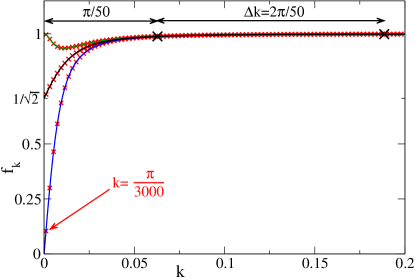
Figure 5: (Color online). Thermodynamic vs. “small system” limit near the Ising critical point. Solid lines correspond to $f_{k}$ calculated for $\gamma=1$, $\delta=0.01$, and – from bottom to top – $c$ equals 0, 1 and 1.5, respectively. Small red crosses mark $f_{k}$’s contributing to fidelity calculated for $N=3000$. Large black crosses show the same, but when the system size is $N=50$. For $N=3000$ the thermodynamic limit is reached. $N=50$ represents the “small system” limit. Notice that in the “small system” limit the resolution in momentum space is insufficient to account for abrupt changes of $f_{k}$ taking place at small momenta.

Still, to see sharp nonanalyticity (i.e. the pinch point) in fidelity when one of the states passes through the critical point we need to have $N\rightarrow\infty$ as demonstrated in Fig. 4. It is caused by discontinuity of $f_{k}$ at zero momentum when $|c|=1$. Indeed, from (11,23,24) it is easy to calculate the limits

$$\begin{array}[]{lr}\lim_{k\to k_{c}}f_{k}=0&{\rm for}~{}|c|<1,\\ \lim_{k\to k_{c}}f_{k}=\frac{1}{\sqrt{2}}&{\rm for}~{}|c|=1,\\ \lim_{k\to k_{c}}f_{k}=1&{\rm for}~{}|c|>1,\end{array}$$ (33)

where $k_{c}=0$ here. This is presented in Figs. 5 and 6. In the latter, it is shown that the jump of $f_{k}$ is roughly happening on the momentum scale given by the inverse of the larger correlation length scaling as $|\delta(|c|-1)|/\gamma$, which is divergent at $|c|\rightarrow 1$ (notice that we have two correlation lengths here for the two ground states entering fidelity). It results in rounding off of the derivative of the scaling parameter $\tilde{d}=-\ln{\cal F}/N$ around the critical point for finite $N$ due to insufficient sampling of $f_{k}$ near $k_{c}=0$. We also notice that the approximation (25) that we make to obtain (27) correctly capture this discontinuity.

Finally, we can discuss errors resulting from our approximations. On the one hand, approximating exact expression for $f_{k}$ (11,23,24) with (25) in the integral (15) leads to ${\cal O}(\delta^{2}/\gamma^{3})$ error in (27). This calculation is quite technical and has been deferred to the Appendix. On the other hand, there are errors connected with estimation of the product (9) by the integral (15). Main contribution here comes from the logarithmic divergence of $\ln f_{k}$ at $k=0$ when

$$|c|<1.$$

It results in a subleading shift which has to be added to the right-hand side of (15). This shift saturates to $\ln 2/2$ when the size of the system $N$ is large enough to well sample the logarithmic singularity. It happens when the system size $N$ is much larger than the larger of the two correlation lengths proportional to $\gamma/|(1-|c|)\delta|$. It can be seen, e.g., when we expand $f_{k}$ to the lowest order in $k$ around $k_{c}=0$,

$$f_{k}\approx\frac{\gamma k}{|\delta|(1-c^{2})},$$ (34)

for $|c|<1$. Using this result we obtain

$$\sum_{0<k<k_{\rm cutoff}}\ln(\alpha k)-\frac{N}{2\pi}\int_{0}^{k_{\rm cutoff}}dk\ln(\alpha k)\overset{N\rightarrow\infty}{=}\frac{\ln 2}{2}.$$ (35)

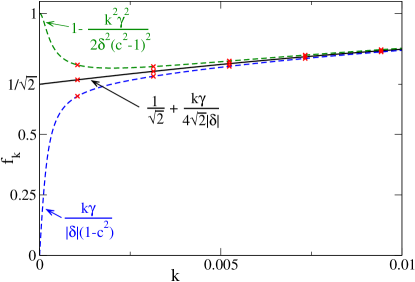
Figure 6: (Color online). Discontinuous change of $f_{k}$ around $c=1$. The curves from bottom to top correspond to $c$ equal to $0.98$, $1$ and $1.02$, respectively. Red crosses, similarly as in Fig. 5, mark $f_{k}$’s contributing to fidelity calculated for $N=3000$. The parameter shift $\delta=0.01$. Lowest order Taylor expansions of $f_{k}$ are listed (but not plotted) for all three curves.

Above, $\alpha=\gamma/|\delta|(1-c^{2})$, $k$’s are given by (10) and $k_{\rm cutoff}$ restricts summation/integration to small momenta for which the expansion (34) is meaningful. We get the equality in (35) in the limit of $k_{\rm cutoff}/\Delta k\to\infty$ when the logarithmic singularity is sampled densely. This can be easily obtained using the Stirling formula.

Including the above discussed errors/corrections into (27) we obtain

$$\frac{\ln\cal F}{N}=\left\{\begin{array}[]{ll}-|\delta|A(c)/\gamma+\ln 2/2N+{\cal O}(\delta^{2}/\gamma^{3})&\ {\rm for}~{}|c|<1,\\ -|\delta|A(c)/\gamma+{\cal O}(\delta^{2}/\gamma^{3})&\ {\rm for}~{}|c|\geq 1,\end{array}\right.$$ (36)

which is equivalent to

$${\cal F}=\left\{\begin{array}[]{cc}\begin{split}&\sqrt{2}\exp\left[-N|\delta|A(c)/\gamma+N{\cal O}(\delta^{2}/\gamma^{3})\right]&{\rm for}~{}|c|<1,\\ &\exp\left[-N|\delta|A(c)/\gamma+N{\cal O}(\delta^{2}/\gamma^{3})\right]&{\rm for}~{}|c|\geq 1.\end{split}\end{array}\right.$$ (37)

Note that the difference between $|c|<1$ and $|c|\geq 1$ cases comes from the lack of a logarithmic singularity in $\ln f_{k}$ in the latter. As illustrated in Fig. 7, numerics compares very well to (36) and (37). The prefactor $\sqrt{2}$ is seen in numerical simulations when $N\gg\gamma/|(1-|c|)\delta|$. In derivation of (36) and (37) we have neglected other errors coming from changing the product (9) into the integral (15). Those corrections are present around $c=\pm 1$ but are subleading and disappear in the limit of $N\rightarrow\infty$ (e.g. they smooth out the pinch point nonanalyticity).

Finally, we would like to stress that a subleading correction to the argument of the exponent in (36), the $\ln 2/2N$ term, increases fidelity by the $\sqrt{2}$ factor (37). Its influence can be neglected when we study the scaling parameter, $-\ln{\cal F}/N$ from (36), instead of fidelity. This is presented in the right column of Fig. 7.

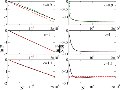
Figure 7: (Color online). Panels in the left and right column illustrate $\ln{\cal F}$ and $\ln{\cal F}/N|\delta|$ as a function of $N$, respectively. From top to bottom rows show results for $c$ equal to $0.9$, $1$ and $1.1$. Black solid lines show numerics. Red dashed lines present $-A(c)N|\delta|$ in the left column and $-A(c)$ in right column. Green dashed-dotted line in the top row shows $-A(c)N|\delta|+\ln 2/2$ in the left panel and $-A(c)+\ln 2/2N|\delta|$ in the right one. See discussion around (36) and (37) for more information about the logarithmic correction. The parameter shift $\delta=10^{-3}$ and $\gamma=1$.

III.2 Across $\gamma$=0 critical line

In this paragraph we follow the path B from Fig. 1, i.e., we substitute into (8)

$$\gamma_{1,2}=\epsilon\pm\delta,\ g_{1,2}=g\in(-1,1),\ \epsilon=c|\delta|.$$ (38)

Two remarks are in order now. First, we shift $\gamma$ instead of $g$ here, but use the same symbols, $\delta$ and $\epsilon$, for the shift as in Sec. III.1. Therefore, some care is required to avoid confusion. Second, critical exponents $z$ and $\nu$ are the same as for the Ising universality class studied in Sec. III.1. Other critical exponents, however, differ between the two transitions Bunder and McKenzie (1999).

Expanding (17) in small $\gamma$ relevant for our calculations, the correlation length reads

$$\xi\sim\gamma^{-1},$$

when $1\gg\gamma<\sqrt{1-g^{2}}$. This can be used to predict the crossover condition from (19). We focus here on large enough $N$ to study the thermodynamic limit. Furthermore, we restrict our calculations to $|\epsilon|,|\delta|\ll\sqrt{1-g^{2}}$ in order to make the problem analytically tractable.

The crucial difference with respect to the calculations from Sec. III.1 is that at the critical points – lying on the $\gamma=0$ and $g\in(-1,1)$ line – the gap in the excitation spectrum (14) closes for momentum

$$k_{c}=\arccos(g).$$ (39)

As can be expected, fidelity in the thermodynamic limit is dominated by contributions coming from momenta centered around $k_{c}$ (Fig. 8).

Putting (38) into (12,13) one gets the following exact expressions

$$p_{k} = (g-\cos k)^{2}+\left(\epsilon^{2}-\delta^{2}\right)\sin^{2}k,$$ (40)

$$q_{k} = 2\delta(g-\cos k)\sin k.$$ (41)

We expand the above around dominant $k_{c}$ to get $p_{k}\approx(1-g^{2})\left((k-k_{c})^{2}+\epsilon^{2}-\delta^{2}\right)$ and $q_{k}\approx(1-g^{2})2\delta(k-k_{c})$, where we have utilized the condition $|\delta|,|\epsilon|\ll\sqrt{1-g^{2}}$. Thus, we get

$$\ln f_{k}\approx\frac{1}{2}\ln\left(\frac{1}{2}+\frac{(k-k_{c})^{2}+\epsilon^{2}-\delta^{2}}{2\sqrt{((k-k_{c})^{2}+\epsilon^{2}-\delta^{2})^{2}+4\delta^{2}(k-k_{c})^{2}}}\right).$$ (42)

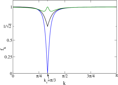
Figure 8: (Color online). Plot of $f_{k}$ for the transition across the $\gamma=0$ line (11). We choose $g=0.5$ and $\delta=0.1$ here. The curves from bottom to top correspond to $c$ equal to $0$, $1$, and $1.5$, respectively. Dominating contribution to fidelity is centered around $k_{c}=\arccos(g)=\pi/3$.

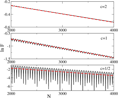
Figure 9: (Color online). Comparison between the smooth part of fidelity (44) – given by the red dashed line – and the exact numerical result (solid black line). In the large $N$-limit and for $|c|>1$ oscillations of fidelity are absent, which is presented here for $c=2$ (top panel). At $c=1$ some oscillations of fidelity are visible for not-too-large-systems (middle panel), but they gradually disappear for large $N$. For $|c|<1$ pronounced oscillations of fidelity surviving in the thermodynamic exist: bottom panel prepared for $c=1/2$. The plots are made for $\delta=0.002$ and $g=0.99$.

We integrate it over $k$ (15), parameterize $\epsilon$ as $c|\delta|$ (note that $\epsilon$ is now the shift of the anisotropy parameter), change the variable $k$ in (15) to $k_{c}+l|\delta|$, and send the new integration limits, $-k_{c}/|\delta|$ and $(\pi-k_{c})/|\delta|$, to $\mp\infty$ respectively.

After all these approximations we arrive at

$$\ln{\cal F}_{\rm smooth}\simeq\frac{N|\delta|}{4\pi}\int_{-\infty}^{\infty}dl\ln\left(\frac{1}{2}+\frac{l^{2}+c^{2}-1}{2\sqrt{(l^{2}+c^{2}-1)^{2}+4l^{2}}}\right).$$ (43)

We have introduced above the symbol ${\cal F}_{\rm smooth}$ because it turns out that for $|c|<1$, i.e. when the two states used to calculate fidelity are obtained on opposite sides of the critical point, there will be oscillatory corrections to fidelity (Fig. 9). Before describing them, we analyze ${\cal F}_{\rm smooth}$.

Except for the integration range, the above integral is exactly the same as the one for the Ising model in (26). Therefore, we obtain

$$\frac{\ln{\cal F}_{\rm smooth}}{N}=-|\delta|2A(c)+{\cal O}\left(\delta^{2}\right),$$ (44)

where $A(c)$ is defined in (28). We estimated numerically the error between the exact integral (15) and the approximated one (43), what is presented in the Appendix. Note that (44) quantifies decay rate of fidelity with system size even when the oscillations are present (Fig. 9).

As pointed out in e.g. Bunder and McKenzie (1999), the anisotropic transition has the same critical behavior as a pair of decoupled Ising chains. This can be seen also through fidelity: there is a prefactor of two in (44) absent in (27) from the previous section. Looking from the momentum space perspective, the factor of two comes from different location of the momentum $k_{c}$. For the Ising model considered in Sec. III.1, $k_{c}=0$ and only $k>k_{c}$ contribute to fidelity (9). Here $k_{c}\neq 0$ and so both $k>k_{c}$ and $k<k_{c}$ add up to fidelity doubling the result [additivity of this effect can be seen from (15)].

We mention also that the pinch point singularity is predicted by (44). It is again visible in momentum space through discontinuity of $f_{k}$ and described by (33): notice that now $k_{c}\neq 0$ (39). This is illustrated in Fig. 8.

Now we are ready to describe the oscillatory corrections to (44) depicted in Fig. 9. These effects, visible for

$$|c|<1,$$

are washed away by the above continuous approximations relying on the limit of $N\to\infty$ that overlooks discretization of momenta $k$. The reason behind the oscillatory behavior is easily identified by looking at Fig. 10. Indeed, fidelity is a product of $f_{k}$’s (9) and as such it is sensitive to the $f_{k}$ factors approaching zero. For $|c|<1$, $f_{k}$’s stay close to zero when $k\approx k_{c}$ (as shown in Fig. 8 this is not the case for $|c|\geq 1$). The arrangement of $k$’s around $k_{c}$ – fixed by discretization (10) – determines fidelity oscillations.

Qualitatively, fidelity reaches its minimum at zero when one of $k$’s equals exactly $k_{c}$. This happens when $k_{c}=(2n+1)\pi/N$ for some integer $n\in[0,N/2-1]$. Then $f_{k=k_{c}}=0$ and a single momentum mode takes fidelity down to zero even for finite $N$. This case is illustrated in Fig. 10a. On the other hand, when $k_{c}$ lays symmetrically between two discretized $k$’s, Fig. 10b, we can expect that fidelity is near its maximum. All other “orientations” of discretized momenta $k$ with respect to $k_{c}$, including the one depicted in Fig. 10c, add to the oscillation presented in the bottom panel of Fig. 9.

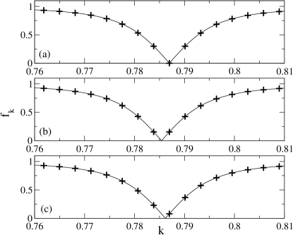
Figure 10: Plot of $f_{k}$ (11) for the transition across the $\gamma=0$ line for $\delta=0.01$, $c=0$ and several values of $g$ such that (a) $k_{c}=\pi\frac{1002}{4000}$, (b) $k_{c}=\pi/4$, and (c) $k_{c}=\pi\frac{1001}{4000}$ [note that $k_{c}$ depends on g (39)]. Pluses mark discretization in momentum space for the size of the system $N=2000$. We see a systematic shift of $f_{k}$’s contributing to fidelity as we slightly change $g$. This results in oscillations of fidelity from the lowest panel of Fig. 9. Parameter $\phi$ from (45) equals $1$, $0$ and $1/2$ for panels (a), (b), and (c), respectively.

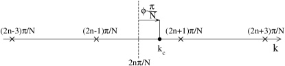
Figure 11: Schematic plot illustrating the shift $\phi$ from (45). Crosses show discretized momenta, the dot denotes position of $k_{c}$ (39), the dashed line goes through the mid point between two discretized momenta being closest to $k_{c}=(2m+\phi)\pi/N$. Note that $\phi>0$ ($\phi<0$) when $k_{c}$ is to the right (left) of the dashed line. Naturally, when $\phi$ approaches $\pm 1$, $k_{c}$ collapses onto one of the discretized $k$’s.

Quantitatively, we introduce the parameter $\phi$ measuring distance of $k_{c}$ from the mid point between two momenta $k$ (10):

$$\phi=\frac{Nk_{c}}{\pi}~{}{\rm modulo}~{}2\in(-1,1].$$ (45)

Its definition is illustrated in detail in Fig. 11. The examples of $\phi=1$, $0$ and $\frac{1}{2}$ are presented in Fig. 10. To extract the oscillatory part we focus on contribution to fidelity coming from momenta around $k_{c}$. Taking the lowest order term of the Taylor expansion of (11) around $k_{c}$ we obtain

$$f_{k}\approx\alpha|k-k_{c}|$$ (46)

where $\alpha=1/|\delta|(1-c^{2})$ is introduced for convenience [compare with (34)]. Without going into details, we define $k_{\rm cutoff}$ estimating the largest $|k-k_{c}|$ for which (46) provides a reasonable approximation to the exact expression for $f_{k}$. Following notation introduced in Fig. 11, we easily find that $f_{k}$ coming from the $m$-th momenta to the left (plus sign) or right (minus sign) of $k_{c}$ equals

$$f_{k}\approx\alpha\frac{\pi}{N}(2m-1\pm\phi).$$

Now we can find how the asymmetry of momenta $k$ around $k_{c}$ modifies fidelity. We do it by factoring out the contributions coming from the $\phi=0$ case where no asymmetry is present. Namely, we calculate

$$\frac{\prod_{k}f_{k}}{\prod_{k}f_{k}|_{\phi=0}}\simeq\prod_{m=1,2,\ldots}^{\frac{N}{\pi}k_{\rm cutoff}}\left[1-\frac{\phi^{2}}{(2m-1)^{2}}\right]\overset{N\rightarrow\infty}{=}\cos\frac{\pi\phi}{2}.$$ (47)

The last equality is reached when $Nk_{\rm cutoff}/\pi\gg 1$. The change of the product into the cosine can be found in Ryz .

To use (47), we notice that for $\phi=0$ fidelity is given by $2{\cal F}_{\rm smooth}$ (44). Thus, for any $\phi$ it is given by $2\cos(\pi\phi/2){\cal F}_{\rm smooth}$ as long as $|c|<1$. The origin of the prefactor of $2$ which multiplies ${\cal F}_{\rm smooth}$ is the same as in Sec. III.1. We have to correct $\ln{\cal F}_{\rm smooth}$ by a subleading term of $\ln 2$ to account for logarithmic singularities of $\ln f_{k}$ near $k_{c}$ (35). Note that for $\phi=0$ the displacement of momenta $k$ around $k_{c}$ is equivalent to displacement of momenta $k$ around $k_{c}=0$ for the Ising model – Sec. III.1. Thus, we can write our final prediction for fidelity in the following form

$${\cal F}=\left\{\begin{array}[]{lr}2\left|\cos\left(\frac{k_{c}N}{2}\right)\right|\exp\left[-N|\delta|2A(c)+N{\cal O}(\delta^{2})\right]&{\rm for}~{}|c|<1,\\ \exp\left[-N|\delta|2A(c)+N{\cal O}(\delta^{2})\right]&{\rm for}~{}|c|\geq 1,\end{array}\right.$$ (48)

where (45) was employed to simplify the oscillating factor. The factor of two and sinusoidal shape of oscillations is reproduced by numerics when the system size $N$ is much larger than the larger of the two correlation lengths proportional to $1/|\delta(1-|c|)|$ (compare to Sec. III.1).

The oscillating part of (48) is illustrated in Fig. 12. As we see in panels (a) and (b), an agreement between (48) and numerics is remarkable. The limits of applicability of (48) are illustrated in panel (c) of Fig. 12. The left part of this panel shows discrepancies resulting from application of (48) to systems whose size $N$ is not much larger than the larger correlation length ($\sim 1/|\delta(1-|c|)|$) – still notice that the period of oscillations is predicted correctly. The right panel reveals that for large enough system sizes, and the very same parameters, the perfect agreement is recovered. We note in passing that those oscillations will survive in the “small system” limit making the fidelity susceptibility approach (3), which assumes that fidelity stays close to unity, inapplicable to this problem.

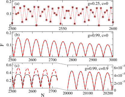
Figure 12: (Color online). Plot of fidelity for the transition across the $\gamma=0$ line for $\delta=0.002$ and various parameters $g$ and $|c|<1$. Black line and crosses show numerical results. Red dashed line and circles show theoretical prediction (48).

We expect that the same mechanism as described above should be able to explain oscillations of fidelity (peaks in fidelity susceptibility) observed in the gapless phase of the Kitaev model Yang et al. (2008).

Finally, it turns out that we can extend the results of this section. The condition $|\delta|,|\epsilon|\ll\sqrt{1-g^{2}}$, which we have been using until now and which is necessary to justify approximations used above, turns out to be too strong. Numerics shows that equation (48) holds for any $|\delta|,|\epsilon|\ll 1$ and $-1<g<1$ when $N$ is large enough.

III.3 On the g=1 critical line

In this paragraph we follow the path C from Fig. 1, i.e., we substitute into (8)

$$\gamma_{1,2}=\epsilon\pm\delta,\ \ g_{1,2}=1.$$ (49)

This choice of the path is much different from what we have considered until now. Indeed, both ground states are calculated at points on the XY phase diagram that lie on the critical line. In particular, it means that the correlation length at any of the points is of the order of the system size $N$.

We start by discussing fidelity calculated away from the multicritical point ($g=1,\gamma=0$). This requires

$$|\delta|\ll|\epsilon|\leq 1.$$

Notice that $\epsilon$ is not assumed to be small here.

The exact expression for fidelity is given by substituting (49) into (9-13). It can be simplified as follows. Since

$$p_{k} = (1-\cos k)^{2}+(\epsilon^{2}-\delta^{2})\sin^{2}k,$$ (50)

$$q_{k} = 2\delta(1-\cos k)\sin k,$$ (51)

for the C path, we see that $p_{k}$ is positive and $q^{2}_{k}/p^{2}_{k}\leq\delta^{2}/(\epsilon^{2}-\delta^{2})$ is small. Expanding $\ln f_{k}$ in $q_{k}/p_{k}$ we obtain

$$\ln f_{k}\simeq-\frac{q_{k}^{2}}{8p_{k}^{2}}.$$

It can be analytically integrated over $k$ from $0$ to $\pi$ (15), and then expanded in $\delta$ to yield

$$\frac{\ln{\cal F}}{N}\simeq-\frac{\delta^{2}}{8|\epsilon|(1+|\epsilon|)^{2}}+{\cal O}(\delta^{4}).$$ (52)

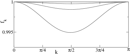
Figure 13: $f_{k}$ along the Ising critical line (49) for $\epsilon=1$ and $\delta=0.05,0.1,0.2$ (top to bottom). The minimum of $f_{k}$ is reached for $k=\arccos\left(\frac{1-\epsilon^{2}+\delta^{2}}{1+\epsilon^{2}-\delta^{2}}\right)\simeq\arccos\left(\frac{1-\epsilon^{2}}{1+\epsilon^{2}}\right)$.

Equation (52) provides an interesting result showing that the universal part of fidelity, present in Secs. III.1 and III.2, is absent here. Therefore, only the nonuniversal part proportional to quadratic displacement of the ground states is present.

Looking at fidelity from the momentum angle, Fig. 13, we notice that $f_{k}$’s are very different here from what we have studied in the previous sections. Not only $f_{k}$’s stay close to unity for all momenta, but also the main contribution to fidelity comes in general from large $k$’s that are not associated with disappearance of the gap: the gap (14) closes at $k_{c}=0$ on this line. This shows that the ground states used to calculate fidelity differ only by the nonuniversal contribution away from the multicritical point. This is to be expected from the renormalization group perspective because we calculate fidelity between states which differ only by an irrelevant variable.

Now we would like to show what happens near the multicritical point and so we assume that

$$|\epsilon|,|\delta|\ll 1,$$

and use the familiar parameterization $\epsilon=c|\delta|$. The dominant contribution to fidelity comes now from momenta around $k_{c}=0$.

Approximating $p_{k}\approx k^{2}(k^{2}/4+\epsilon^{2}-\delta^{2})$ and $q_{k}\approx k^{3}\delta$ from (50,51) and using the same methods as in Sec. III.1, we obtain

$$\ln{\cal F}=\left\{\begin{array}[]{cc}\begin{split}&-N\left[|\delta|2A(c)+{\cal O}(\delta^{2})\right]+\ln 2/2&{\rm for}~{}|c|<1,\\ &-N\left[|\delta|2A(c)+{\cal O}(\delta^{2})\right]&{\rm for}~{}|c|\geq 1,\end{split}\end{array}\right.$$ (53)

where the scaling function $A(c)$ is given by (28).

This is a pretty interesting result showing that despite the fact that the ground states entering fidelity are calculated on the critical line, there is a universal contribution to fidelity. This contribution can be traced back to the multicritical point: the dominant critical point on the $g=1$ line. Evidence for that is twofold. First, the universal result (53) appears as we approach the multicritical point. Second, the scaling exponent $\nu$, that can be extracted from (53) by comparing it to (4), equals $1$. It matches the predicted value for this multicritical point along the $g=1$ line/direction Mukherjee et al. (2011). It should be also mentioned that the concept of the dominant critical point has been introduced in Deng et al. (2008) in the context of quench dynamics.

Finally, it is interesting to see how (53) crosses over into (52) as we go away from the multicritical point (the limit of $|c|\gg 1$). Assuming that $|\delta|\ll|\epsilon|\ll 1$, equation (53) can be simplified to

$$\frac{\ln{\cal F}}{N}\simeq-\frac{\delta^{2}}{8|\epsilon|},$$

which matches (52) in the leading order in $\epsilon$. Note, however, that one cannot apply (53) to arbitrary distances away from the critical point because it is valid for $|\epsilon|=|c\delta|\ll 1$ only. For larger $\epsilon$’s non-universal contributions dominate fidelity (52).

III.4 Near $\gamma$=0 and g=1: multicritical point

In this paragraph we follow the path D from Fig. 1, i.e., we substitute into (8)

$$g_{1,2}=1+\epsilon\pm\delta,\ \gamma_{1,2}=\alpha(\epsilon\pm\delta),\ \epsilon=c|\delta|,$$ (54)

where $0<\alpha<\infty$ is the slope of our path. We restrict our studies to $g_{1,2}\geq 1$ and $\gamma_{1,2}\geq 0$: both ground states used to calculate fidelity are obtained on the paramagnetic side (Fig. 1). This requires $\epsilon\geq|\delta|$ or equivalently $c\geq 1$. Fidelity calculated along this path is “influenced” by the multicritical point at $g_{c}=1$ and $\gamma_{c}=0$.

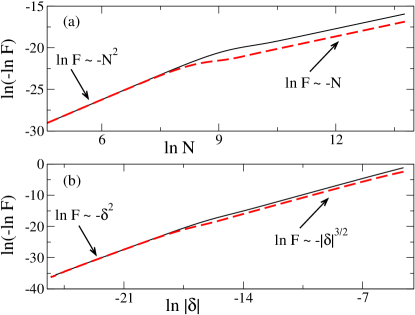
Figure 14: (Color online). Transition from the “small system” limit to the thermodynamic limit near the multicritical point located at $g=1$ and $\gamma=0$. (a): the transition as a function of the system size $N$ at fixed $\delta=10^{-8}$. (b): the transition as a function of parameter difference $\delta$ at fixed $N=3000$. In both plots solid (black) line shows fidelity for $c=1$, i.e., ${\cal F}=|\langle 1,0|1+2\delta,2\delta\rangle|$, while the dashed (red) line shows the $c=5$ case, i.e., ${\cal F}=|\langle 1+4\delta,4\delta|1+6\delta,6\delta\rangle|$ (54). Note that $\alpha=1$ is assumed here.

The condition for the crossover between the “small system” limit and the thermodynamic limit near the multicritical point reads (19)

$$N|\delta|^{\nu}\sim 1.$$ (55)

As we deal here with a multicritical point that is characterized by more than one divergent length scale, it is important to carefully verify the above prediction to make sure that the relevant $\nu$ is used in (55).

The crossover is illustrated in Fig. 14, where distinct scalings of fidelity with either the system size $N$ or the parameter difference $\delta$ are easily observed. In Fig. 14a the parameter difference $\delta$ is kept constant and the system size $N$ is varied. We see that for small system sizes $\ln{\cal F}\sim-N^{2}$, while for large ones $\ln{\cal F}\sim-N$. In Fig. 14b the system size $N$ is kept constant, while the parameter shift $\delta$ is varied. Again two regimes appear: for small $\delta$ we have $\ln{\cal F}\sim-\delta^{2}$, while for larger $\delta$ we get $\ln{\cal F}\sim-|\delta|^{3/2}$.

The location of the crossover can be studied in exactly the same way as in Sec. III.1. Briefly, as the system size $N$ is increased in Fig. 14a, the slope of $\ln(-\ln{\cal F})$ changes smoothly from $2$ (corresponding to $\ln{\cal F}\sim-N^{2}$) to $1$ (corresponding to $\ln{\cal F}\sim-N$). The crossover region between the two limits is centered around $N=N_{3/2}$ where the local slope equals $3/2$. By repeating the calculation from Fig. 14 for various $\delta$’s we have numerically obtained $N_{3/2}(\delta)$. A power-law fit described in Fig. 15a reveals that $N_{3/2}\sim 1/\sqrt{|\delta|}$ supporting $\nu=1/2$ in (55). Similar analysis can be performed on data from Fig. 14b. Indeed, now we look at $\delta_{7/4}(N)$ such that the slope of $\ln(-\ln{\cal F})$ equals $7/4$, i.e., is half-way between $2$ and $3/2$ observed on both “ends” of Fig. 14b. Fig. 15b, where the power-law fit is performed, shows that $\delta_{7/4}\sim N^{-2}$ again pointing to $\nu=1/2$. Therefore, we conclude that the crossover condition (55) holds near the multicritical point with $\nu=1/2$ on the paramagnetic side.

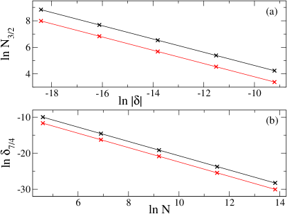
Figure 15: (Color online). Numerical study of the crossover condition (55). Crosses come from numerics (see text for details), while straight lines are linear fits Fit . In both panels upper (lower) data sets correspond to $c=1$ ($c=5$). Panel (a): we fit $a$ and $b$ coefficients of $\ln N_{3/2}=a+b\ln\delta$. For $c=1$ ($c=5$) we obtain $b=-0.499\pm 0.0003$ ($b=-0.4992\pm 0.0005$). Panel (b): we fit $a$ and $b$ coefficients of $\ln\delta_{7/4}=a+b\ln N$. For $c=1$ ($c=5$) we obtain $b=-1.989\pm 0.005$ ($b=-1.9987\pm 0.0008$). The numerics for these plots is done with $\alpha=1$. The fitting coefficient $a$ is not listed as it is of minor interest.

We focus on the thermodynamic limit again. Substituting (54) into (12,13) we obtain

$$p_{k} = (1+\epsilon-\cos k)^{2}-\delta^{2}+\alpha^{2}(\epsilon^{2}-\delta^{2})\sin^{2}k,$$

$$q_{k} = 2\alpha\delta(1-\cos k)\sin k.$$

When both points – $(g_{1},\gamma_{1})$ and $(g_{2},\gamma_{2})$ (54) – are on the paramagnetic side, then $p_{k}>0$ and $q^{2}_{k}/p^{2}_{k}<\alpha|\delta|/2\ll 1$ is a small parameter in which we expand $\ln f_{k}$. This brings us again to

$$\ln f_{k}\simeq-\frac{q_{k}^{2}}{8p_{k}^{2}}.$$ (56)

Integrating (56) over $k$ from $0$ to $\pi$ (15), and then expanding the resulting expression in $\delta$ we get

$$\frac{\ln{\cal F}}{N}=-|\delta|^{3/2}\alpha^{2}A_{\rm MCP}(c)+\delta^{2}\alpha^{2}/4+{\cal O}(|\delta|^{5/2}).$$ (57)

The scaling function for the multicritical point is given by

$$A_{\rm MCP}(c)=\frac{(c+1)^{3/2}(3-2c)+(c-1)^{3/2}(3+2c)}{16\sqrt{2}},$$

which is valid for $c\geq 1$. This result is illustrated in Fig. 16, where small enough $\delta$ has been chosen to keep the terms ${\cal O}(|\delta|^{5/2})$ negligible. We assume such choice of $\delta$ from now on. The result (57) is interesting for several reasons.

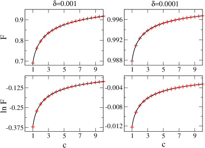
Figure 16: (Color online). Comparison between numerics (solid lines) and analytics [pluses given by (57)]. In all panels $N=10^{5}$ and $\alpha=1$. The parameter shift $\delta$ is chosen to be small enough to keep the ${\cal O}(|\delta|^{5/2})$ corrections to (57) negligible.

First, the exponent $3/2$ does not fit the expected $d\nu$ value from (4): neither $\nu=1/2$ nor $\nu=1$, both considered near the multicritical point Mukherjee et al. (2011), agree here. Explanation of that anomaly is beyond the scope of this work.

Second, due to remarkable simplicity of (57) we can analyze in detail the interplay between the nonanalytic and the subleading contribution to fidelity. The nonanalytic term dominates over the subleading one when

$$|\delta|^{3/2}\alpha^{2}A_{\rm MCP}(c)\gg\delta^{2}\alpha^{2}/4\Rightarrow|\delta|\ll 16A_{\rm MCP}(c)^{2}\leq 1/4.$$

Additionally, the “thermodynamic limit” condition $N\sqrt{\delta}\gg 1$ must be satisfied so that (57) holds. If these two conditions are fullfield, $\ln{\cal F}\approx-N|\delta|^{3/2}\alpha^{2}A_{\rm MCP}(c)$. This does not, however, guarantee that ${\cal F}$ is well approximated by $\exp(-N|\delta|^{3/2}\alpha^{2}A_{\rm MCP}(c))$. Indeed, the latter requirement puts an additional bound on the parameter shift $\delta$:

$$N\delta^{2}\alpha^{2}/4\ll 1\Rightarrow\exp(N\delta^{2}\alpha^{2}/4)\approx 1.$$

All these conditions can be simultaneously satisfied.

Third, equation (57) shows that fidelity near the multicritical point – at least in the paramagnetic phase discussed here – does not have to be small in the thermodynamic limit. This is in stark contrast to what we found near the Ising critical point, where the thermodynamic-limit condition (20) implied smallness of ${\cal F}$ (27). Here, we can have $N\sqrt{|\delta|}\gg 1$ and still $\exp(-N|\delta|^{3/2}\alpha^{2}A_{\rm MCP}(c)+N\delta^{2}\alpha^{2}/4)$ anywhere between $0$ and $1$.

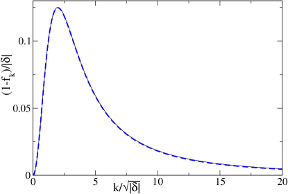
Figure 17: (Color online). We show here from the momentum space angle that $\ln{\cal F}\sim-|\delta|^{3/2}$ (57). We plot the rescaled $f_{k}$ functions for $c=1$ and $\alpha=1$: one for $\delta=0.001$ (solid black line) and the other for $\delta=0.01$ (dashed blue line). As the two curves overlap very well, we see that $(1-f_{k})/|\delta|=h(k/\sqrt{|\delta|})$, where $h$ is some non-singular function. This implies that $\ln{\cal F}\sim\int dk\ln f_{k}\sim-|\delta|^{3/2}$ ($f_{k}\approx 1$ so we approximate $\ln f_{k}\simeq f_{k}-1$). This confirms leading scaling of (57) with $\delta$ and independently confirms the condition (55) with $\nu=1/2$. We also note that these rescalings work in the limit of $\delta\to 0$.

Fourth, similarly as in the Ising chain one can easily derive from (57) transition to the analytic limit in $\delta$ far away from the critical point. Considering $\epsilon\gg|\delta|$ or simply $c\gg 1$ (but still $\epsilon=c|\delta|\ll 1$), $A_{\rm MCP}(c)\simeq 5/32\sqrt{2c}$ and so

$${\cal F}\simeq\exp\left(-\delta^{2}N\frac{5\alpha^{2}}{32\sqrt{2\epsilon}}\right).$$ (58)

This is again a new result. If we expand (58) assuming that the argument under the exponent is small, we get a fidelity susceptibility-like expression in the thermodynamic limit

$${\cal F}\simeq 1-\delta^{2}\chi_{F}/2,\ \ \chi_{F}\approx N\frac{5\alpha^{2}}{16\sqrt{2\epsilon}}.$$

The above equation can be also obtained when we start with (3) and expand the resulting expression for $\chi_{F}$ in $\epsilon$. It predicts that fidelity susceptibility away from the multicritical point in the paramagnetic phase scales as $\epsilon^{-1/2}$.

Finally, we mention that one can find the $|\delta|^{3/2}$ scaling of $\ln{\cal F}$ by looking directly at $f_{k}$. This is explained in Fig. 17.

IV Extended Ising model

In this section we consider the Hamiltonian Wolf et al. (2006)

$$\hat{H} = \sum_{n=1}^{N}\left[-2(1-g^{2})\sigma_{n}^{x}\sigma_{n+1}^{x}-(1+g)^{2}\sigma_{n}^{z}\right.$$ (59)

$$~{}~{}~{}~{}~{}~{}+\left.(1-g)^{2}\sigma_{n}^{x}\sigma_{n+1}^{z}\sigma_{n+2}^{x}\right].$$

with periodic boundary conditions $\sigma_{n+N}=\sigma_{n}$. Its ground state is given exactly by finite rank Matrix Product State Wolf et al. (2006). It has the critical point at $g_{c}=0$, which is characterized by the critical exponents $\nu=1$ and $z=2$. In contrast to the Ising model, neither entropy of entanglement nor the ground state energy is singular at this critical point. Still, as we will see below, the basic features of that transition are captured by fidelity. Introducing the notation $|g\rangle$ for the ground state of (59), and defining ${\cal F}$ as $|\langle g_{1}|g_{2}\rangle|$ one obtains that

$${\cal F}=\frac{\left|(1+\sqrt{g_{1}g_{2}})^{N}+(1-\sqrt{g_{1}g_{2}})^{N}\right|}{\sqrt{(1+g_{1})^{N}+(1-g_{1})^{N}}\sqrt{(1+g_{2})^{N}+(1-g_{2})^{N}}}.$$ (60)

This is an exact expression from Cozzini et al. (2007); Zhou and Barjaktarevič (2008). We are going to simplify this result to discuss it from the perspective relevant for our approach.

We follow notation from Sec. III writing

$$g_{1}=\epsilon+\delta,\ g_{2}=\epsilon-\delta,\ \epsilon=c|\delta|.$$ (61)

We stay close to the critical point so that $|\delta|,|\epsilon|\ll 1$ and approximate (60) with hyperbolic functions

$${\cal F}\simeq\frac{\left|\cosh\left(N\sqrt{\epsilon^{2}-\delta^{2}}\right)\right|}{\sqrt{\cosh\left(N(\delta+\epsilon)\right)\cosh\left(N(\epsilon-\delta)\right)}}.$$ (62)

This simple expression allows us to easily study the “small system” limit and the thermodynamic limit.

First, we focus on the “small system” limit, say $\delta\to 0$ at fixed $N$ for simplicity. Expansion of (62) in $\delta$, the fidelity susceptibility approach (3), results in

$${\cal F}\simeq 1-\frac{\delta^{2}N^{2}}{2}\left[\frac{1}{\cosh^{2}(\epsilon N)}+\frac{\tanh(\epsilon N)}{\epsilon N}\right].$$ (63)

This expression depends on two parameters: $N|\delta|$ and $N|\epsilon|$. As we keep the former small, we can focus on its $N|\epsilon|$ dependence. When $|\epsilon|N\ll 1$ then (63) simplifies to

$${\cal F}\simeq 1-\delta^{2}N^{2}$$

reproducing expected scaling of fidelity susceptibility at the critical point Schwandt et al. (2009); Albuquerque et al. (2010); Barankov (2009); De Grandi et al. (2010a, b); Pol . In the opposite limit of $|\epsilon|N\gg 1$, (63) can be written as

$${\cal F}\simeq 1-\delta^{2}N/2|\epsilon|.$$ (64)

This again agrees with the scaling predictions Schwandt et al. (2009); Albuquerque et al. (2010); Barankov (2009); De Grandi et al. (2010a, b); Pol . Finally, note that when (63) holds, fidelity stays very close to unity.

Second, we concentrate on the thermodynamic limit, say $N\rightarrow\infty$ at fixed $\delta$, where we obtain from (62)

$${\cal F}\simeq\left\{\begin{array}[]{cl}\begin{split}&2\left|\cos\left(|\delta|N\sqrt{1-c^{2}}\right)\right|\exp\left(-|\delta|N\right)&{\rm for}~{}|c|<1,\\ &\sqrt{2}\exp\left(-|\delta|N\right)&{\rm for}~{}|c|=1,\\ &\exp\left(-|\delta|N\left(|c|-\sqrt{c^{2}-1}\right)\right)&{\rm for}~{}|c|>1.\end{split}\end{array}\right.$$ (65)

To be more precise, we mention that (65) provides a good approximation to the exact result when $\max\left[N|\epsilon+\delta|,N|\epsilon-\delta|\right]\gg 1$, which is a thermodynamic limit condition based on (19).

Similarly as for the XY model, we introduce the scaling function $A_{MPS}(c)$ as

$$A_{MPS}(c)=\left\{\begin{array}[]{c}\begin{split}&1&{\rm for}~{}|c|\leq 1,\\ &|c|-\sqrt{c^{2}-1}&{\rm for}~{}|c|>1.\end{split}\end{array}\right.$$ (66)

$A_{MPS}(c)$ is nonanalytic when $|c|=1$, i.e., when one of the states is exactly at the critical point, signaling the pinch point singularity Zhou and Barjaktarevič (2008); Zhou et al. (2008a, b). As expected, this singularity is rounded off in finite systems.

When $|c|\gg 1$, or equivalently $|\delta|\ll|\epsilon|\ll 1$, then the scaling function $A_{MPS}$ approaches zero as $1/2|c|$ leaving us with

$${\cal F}\simeq\exp\left(-\delta^{2}N/2|\epsilon|\right).$$

This coincides with the fidelity susceptibility result (64) when the argument of the exponent is small, but provides a different result otherwise.

Now we will study the origin of oscillations and prefactors appearing in (65) illustrating how the analytical techniques from Sec. III can be applied to other models as well. Hamiltonian (59) can be diagonalized using exactly the same formalism as in Sec. III. Indeed, the Jordan-Wigner transformation translates (59) into a chain of noninteracting fermions which can be solved using Fourier and Bogoliubov transformations. We assume even $N$ and follow notation from Dziarmaga (2005) during diagonalization of (59). The ground state lays then in a subspace with even number of quasiparticles. In that subspace the Hamiltonian (59) is diagonalized to the form $\hat{H}=\sum_{k>0}\epsilon_{k}\left(\gamma_{k}^{\dagger}\gamma_{k}+\gamma_{-k}^{\dagger}\gamma_{-k}-1\right)$, where $\gamma_{k}$ are the fermionic annihilation operators and the energy gap is given by

$$\epsilon_{k}=4\left(1+g^{2}-(1-g^{2})\cos k\right).$$

It reaches zero at the critical point $g_{c}=0$ for $k_{c}=0$. For small $k$ and $g$ we can approximate $\epsilon_{k}\approx 8g^{2}+2k^{2}$, which confirms the critical exponents $\nu=1$ and $z=2$ (at the critical point the gap scales as $k^{z}$, while near the critical point it closes as $|g-g_{c}|^{z\nu}$).

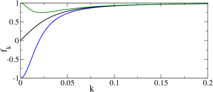
Figure 18: (Color online). The lines correspond to $f_{k}$ plotted for $\delta=0.01$ (69). From bottom to top $c$ equals $0$, $1$ and $1.5$, respectively. For $c=0$ the ground states entering fidelity are calculated on the opposite sides of the critical point, for $c=1$ one of them is obtained at the critical point, while for $c=1.5$ they are both obtained on the same side of the critical point.

Fidelity is given by ${\cal F}=\prod_{k>0}\left|\cos(\theta^{1}_{k}/2-\theta^{2}_{k}/2)\right|$, where this time $\theta^{i}_{k}$’s are defined by

$$\tan\theta^{i}_{k}=\frac{2(1-g_{i}^{2})\sin k-(1-g_{i})^{2}\sin 2k}{(1+g_{i})^{2}-2(1-g_{i}^{2})\cos k+(1-g_{i})^{2}\cos 2k}.$$

After some algebra we arrive at

$${\cal F} =\prod_{k>0}|f_{k}|,$$ (67)

$$k =(2n+1)\pi/N,\ n=0,1,\ldots,N/2-1,$$ (68)

$$f_{k} =\frac{p_{k}}{\sqrt{p_{k}^{2}+q_{k}^{2}}},$$ (69)

$$p_{k} =1+g_{1}g_{2}-(1-g_{1}g_{2})\cos k,$$ (70)

$$q_{k} =(g_{1}-g_{2})\sin k.$$ (71)

For the sake of presentation we allow $f_{k}$ to take negative values here and use the parameterization (61). The prototypical behavior of $f_{k}$ is shown in Fig. 18.

We expand $p_{k}$ and $q_{k}$ around $k_{c}=0$ and for $|\epsilon|,|\delta|\ll 1$ we get $p_{k}\approx k^{2}/2+2(\epsilon^{2}-\delta^{2})$ and $q_{k}\approx 2\delta k$. Thus we can approximate

$$\ln|f_{k}|\approx\frac{1}{2}\ln\left(\frac{(k^{2}/4+\epsilon^{2}-\delta^{2})^{2}}{(k^{2}/4+\epsilon^{2}-\delta^{2})^{2}+(\delta k)^{2}}\right).$$ (72)

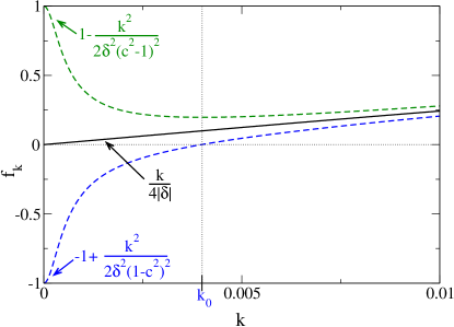
Figure 19: (Color online). Discontinuous change of $f_{k}$ around $c=1$. The curves from bottom to top correspond to $c$ equal to $0.98$, $1$ and $1.02$, respectively. The parameter shift $\delta=0.01$. Lowest order Taylor expansions of $f_{k}$ around $k_{c}=0$ are listed (but not plotted) for all three curves. When $|c|<1$ then $f_{k}$ crosses zero for $k_{0}\neq 0$.

Before we discuss $f_{k}$ in details, we start the calculation of fidelity by approximating the product in (67) by an integral. Similarly as in Sec. III.2 we introduce $\ln{\cal F}_{\rm smooth}=\frac{N}{2\pi}\int_{0}^{\pi}dk\ln|f_{k}|$. In order to calculate it we use approximation (72), change the variable $k$ into $|\delta|l$ and send the new upper integration limit, $\pi/|\delta|$, to infinity. This yields

$$\ln{\cal F}_{\rm smooth}\simeq\frac{N}{4\pi}|\delta|\int_{0}^{\infty}dl\ln\left(\frac{(l^{2}/4+(c^{2}-1))^{2}}{(l^{2}/4+(c^{2}-1))^{2}+l^{2}}\right).$$

The last integral can be calculated analytically:

$$\frac{\ln{\cal F}_{\rm smooth}}{N}=-|\delta|A_{MPS}(c)+{\cal O}(\delta^{2}),$$ (73)

where $A_{MPS}(c)$ is defined by (66). We notice that smooth (continuous) representation of fidelity reproduces leading exponential decay from (65). It also agrees with the general scaling results (4) and (5). The ${\cal O}(\delta^{2})$ error in the integral can be verified numerically in a similar way as described in the Appendix.

As noticed earlier, $A_{MPS}(c)$ is nonanalytic for $|c|=1$. This is also visible from momentum space perspective through discontinuity of $f_{k}$ at $k_{c}=0$ and $|c|=1$. Indeed, it is easy to check that

$$\begin{array}[]{lr}\lim_{k\to k_{c}}f_{k}=-1&{\rm for}~{}|c|<1,\\ \lim_{k\to k_{c}}f_{k}=0&{\rm for}~{}|c|=1,\\ \lim_{k\to k_{c}}f_{k}=1&{\rm for}~{}|c|>1.\end{array}$$

This discontinuity is presented in detail in Fig. 19.

Appearance of oscillations and some constant prefactors in (65), overlooked by “continuous” ${\cal F}_{\rm smooth}$, can be explained in a similar way as in Secs. III.1 and III.2. Again they can be traced back to the fact that $f_{k}$ crosses zero when $|c|\leq 1$ (Fig. 18). This leads to logarithmic divergence of $\ln|f_{k}|$ causing corrections to ${\cal F}_{\rm smooth}$.

More quantitatively, when $|c|=1$ then $f_{k}$ reaches zero for $k=k_{c}=0$. Similarly as in Sec. III.1 it leads to the additional term, saturating at $\ln 2/2N$, which has to be added to the right-hand side of (73). It results in the prefactor of $\sqrt{2}$ in (65). When $|c|<1$, $f_{k}$ reaches zero for $k_{0}\neq 0$, which is different than $k_{c}=0$ for which the gap closes. It is easy to check that

$$k_{0}=\arccos\left(\frac{1-\delta^{2}(1-c^{2})}{1+\delta^{2}(1-c^{2})}\right)\simeq 2|\delta|\sqrt{1-c^{2}}.$$ (74)

This $k_{0}$ is in general incommensurate with momenta $k$ (68) and it leads to oscillations of fidelity. We can directly use the formalism presented in Sec. III.2 to obtain the additional factor of $2\left|\cos(k_{0}N/2)\right|\approx 2\left|\cos(|\delta|N\sqrt{1-c^{2}})\right|$ modifying ${\cal F}_{\rm smooth}$. Note that this is the prefactor appearing in (65) and that the approximation (74) has been used to simplify $\cos(k_{0}N/2)$.

V Fidelity and nonequilibrium quantum quenches

Our goal here is to briefly illustrate how our results and analytical techniques presented in the previous sections can contribute to a better theoretical description of quantum quenches (both instantaneous and continues ones).

The simplest quench one can consider is the instantaneous quench, where the parameter of the Hamiltonian, say $\lambda$, is changed at once from $\lambda_{1}$ to $\lambda_{2}$. Assuming that the system was initially prepared in the ground state $|\lambda_{1}\rangle$, the modulus of the overlap of its wave-function onto the new ground state $|\lambda_{2}\rangle$ reads (1)

$$|\langle\lambda_{1}|\lambda_{2}\rangle|={\cal F}(\lambda_{1}/2+\lambda_{2}/2,\lambda_{2}/2-\lambda_{1}/2).$$ (75)

In other words, fidelity provides here a square root of the probability of finding the system in the new ground state after the instantaneous quench. If the system is in the thermodynamic limit and $\delta=\lambda_{1}/2-\lambda_{2}/2$ is small enough, depending on $\lambda=\lambda_{1}/2+\lambda_{2}/2$ either (4) or (5) can be used to evaluate (75) near the critical point ($\lambda\approx\lambda_{c}$).

Another application of the analytical techniques developed in the former sections comes in the context of the density of quasiparticles excited during an instantaneous quench De Grandi et al. (2010a, b); Pol . For clarity of our discussion we will focus here on the instantaneous transition in the Ising model, where the system is suddenly moved from $(g_{1},\gamma_{1})$ to $(g_{2},\gamma_{2})$ with $g_{1,2}=1+\epsilon\pm\delta$ and $\gamma_{1,2}=1$ (path A on Fig. 1; see (6) for the Hamiltonian). The density of quasiparticles reads

$$n_{ex}=\int_{0}^{\pi}\frac{dk}{\pi}~{}p^{\rm ex}_{k}=\int_{0}^{\pi}\frac{dk}{\pi}(1-f_{k}^{2})=|\delta|B(c)+{\cal O}(\delta^{2}),$$ (76)

where $p_{k}^{\rm ex}$ is the probability of excitation of the $k$-th momentum mode during the quench Pol ; Deng et al. (2011), $f_{k}$ is related to fidelity (75) through (9-13), and again we assume $|\delta|$, $|\epsilon|\ll 1$ and $c=\epsilon/|\delta|$.

The scaling function $B(c)$ – presented in Fig. 20a – is given by

$$B(c)=\frac{1}{2\pi}\left\{\begin{array}[]{ll}\begin{split}&(1-|c|){\rm Im}E(c_{2})+2K(c_{1})&{\rm for}~{}|c|<1,\\ &(|c|-1){\rm Im}E(c_{2})-2K(c_{1})&{\rm for}~{}|c|\geq 1,\end{split}\end{array}\right.$$ (77)

where $c_{1}$, $c_{2}$, $K$ and $E$ are given by (29) and (30). To obtain this result we used the approximation (25).

Equation (76) extends the results of Pol where density of excited quasiparticles $n_{ex}$ was calculated for a specific situation where the instantaneous quench has either began from the critical point or ended at the critical point. Note that we consider the instantaneous quench everywhere around the critical point. Moreover, our calculation provides the scaling function $B(c)$, which is indispensable for capturing full universal description of $n_{ex}$ for any two states close to the critical point. It also allows for unified description of the density of quasiparticles for instantaneous quenches both near and away from the critical point. To illustrate the latter, we consider $|c|\gg 1$, but still $|\delta|\ll|\epsilon|\ll 1$, and expand (77) getting $B(c)\simeq 1/4|c|$. Putting it into (76) we obtain

$$n_{ex}\simeq\delta^{2}/4|\epsilon|.$$

We also note that the scaling function $B(c)$ is nonanalytic for $|c|=1$. This results from discontinuity of $f_{k}$, and consequently $p_{k}^{\rm ex}$, at $k_{c}=0$ and $|c|=1$ (33). Indeed, the derivative of $B(c)$ can be expanded around $c=1$

$$\left.\frac{dB(c)}{dc}\right|_{c\rightarrow 1}=\frac{2-3\ln 2}{2\pi}+\frac{\ln|1-c|}{2\pi}+{\cal O}(c-1).$$ (78)

This logarithmic divergence is reached when the size of the system $N\rightarrow\infty$ (see Fig. 20b and the related discussion in Sec. III.1).

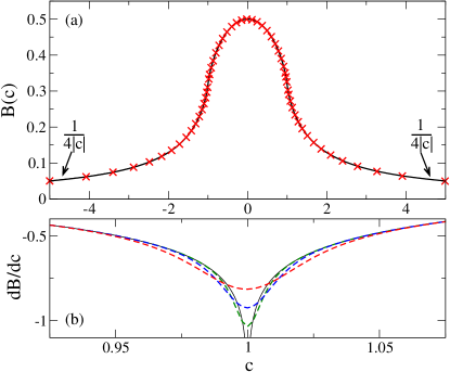
Figure 20: (Color online). Scaling function (77), and its derivative (78), characterizing density of quasiparticles after an instantaneous quench in the Ising model (76). Panel (a): the black line shows analytical expression (77), while red crosses show numerically evaluated $n_{ex}/|\delta|$ from (76) for $N=10^{5}$ and $\delta=10^{-3}$. Panel (b): logarithmic divergence of $dB(c)/dc$ around $c=1$ (78). The solid black line shows analytical result (78). The dashed lines present numerics done for $\delta=10^{-3}$ and $N$ equal to $10^{5}$ (red), $2\times 10^{5}$ (blue) and $4\times 10^{5}$ (green) [top to bottom]. The logarithmic singularity is reached in the limit of $N\rightarrow\infty$ (compare with Fig. 4 and discussion in Sec. III.1).

A more complicated quench dynamics shows when the parameter driving the transition, say $\lambda$, is gradually shifted

$$\lambda(t)=\lambda_{c}+t/\tau_{Q},\ \ t=-\infty\dots\infty,$$

where the quench time scale $\tau_{Q}$ controls how fast the system is driven: see Dziarmaga (2010) for a review of the resulting quantum dynamics from the perspective relevant for our discussion. Briefly, it turns out that the system’s evolution can be approximately divided into three regimes (Fig. 21) Damski (2005); Zurek et al. (2005). First, the adiabatic regime takes place as long as the system is far enough from the critical point: $\lambda(t)\leq\lambda_{c}-\hat{\lambda}$, where $\hat{\lambda}$ is a small parameter that will be discussed below. Assuming that the evolution started from a ground state, wave-function of the driven system is given here by the instantaneous ground state of its Hamiltonian. Then the impulse (diabatic) regime happens around the critical point, $\lambda(t)\in(\lambda_{c}-\hat{\lambda},\lambda_{c}+\hat{\lambda})$, and system’s wave-function is assumed not to change here. Therefore, it is the same as at the last “adiabatic” instant $\hat{t}$ such that $\lambda(-\hat{t})=\lambda_{c}-\hat{\lambda}$. Finally, the system enters the second adiabatic regime when $\lambda(t)\geq\lambda_{c}+\hat{\lambda}$. It is assumed that no additional excitations are created by the quench in this regime. The parameter $\hat{\lambda}$ is provided by the quantum version of the Kibble-Zurek theory Dziarmaga (2010)

$$\hat{\lambda}\sim\tau_{Q}^{-1/(1+z\nu)},$$

where $\tau_{Q}\gg 1$ is assumed (the slow quench limit) and the prefactor omitted above is ${\cal O}(1)$: $\hat{\lambda}\ll 1$. In addition, one also assumes here that the correlation length ($\xi$) during the quench is much smaller than the system size to avoid finite size effects. In the adiabatic-impulse approximation this implies that $L\gg\xi(\lambda_{c}-\hat{\lambda})\sim\hat{\lambda}^{-\nu}$ or simply $N/\tau_{Q}^{d\nu/(1+z\nu)}\gg 1$, where $N=L^{d}$.

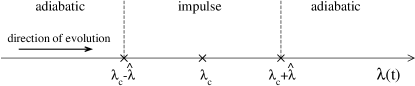
Figure 21: Schematic illustration of dynamics of a generic quantum phase transition (see text for details).

It turns out that one can relate all these concepts to fidelity and use (4) to quantify scaling of the system excitation with the quench rate $\tau_{Q}$. Employing the adiabatic-impulse approximation, we see that the population left in the instantaneous ground state away from the critical point – i.e., after leaving the impulse regime – is given by

$$|\langle\lambda_{c}-\hat{\lambda}|\lambda_{c}+\hat{\lambda}\rangle|^{2}={\cal F}^{2}(\lambda_{c},\delta),\ \ \delta\sim\tau_{Q}^{-1/(1+z\nu)},$$

or, after using (4), by

$$\exp\left(-N\times{\rm const}/\tau_{Q}^{d\nu/(1+z\nu)}\right),$$ (79)

where the ${\rm const}$ prefactor is given by ${\cal O}(2A(0))$. This result has a simple interpretation in the context of symmetry breaking phase transitions. As predicted by the Kibble-Zurek theory, such transitions lead to creation of topological defects whose density is given by $\tau_{Q}^{-d\nu/(1+z\nu)}$ Dziarmaga (2010). Thus, the probability of finding the system after the quench in its instantaneous ground state is exponential in the number of topological defects created during the quench (see Sec. V of Cincio et al. (2009) for the same conclusion worked out in the Ising model; note that (79) is much smaller than unity when the adiabatic-impulse approximation applies).

This is in agreement with studies of dynamics of the quantum Ising chain, whose Hamiltonian is given by (6) with $\gamma=1$ (note that $g$ in (6) corresponds to $\lambda$ here) Cincio et al. (2009); Dziarmaga (2005). In Sec. V of Cincio et al. (2009) the Ising chain was initially exposed to a large magnetic field: evolution begun from a paramagnetic phase ground state. The magnetic field was ramped down on a time scale $\tau_{Q}$ and the system was moved across the paramagnetic-ferromagnetic critical point. The evolution stopped at the zero magnetic field (deeply in the second adiabatic regime) and the squared overlap between the evolved wave-function and the ground state at the zero magnetic field was found to equal

$$\exp\left(-N\times{\rm const}/\sqrt{\tau_{Q}}\right),$$

where ${\rm const}={\cal O}(1)$. This is in agreement with (79) because $\nu=z=d=1$ for the quenched Ising model. Naturally, it would be also interesting to verify our simple scaling result (79) in other models as well.

At the risk of laboring the obvious, we note that fidelity – or more interestingly the scaling factor $\tilde{d}$ (31) – is insensitive to both the relaxation processes after the instantaneous quench and the adiabatic dynamics following crossing of the critical point. This shall make it a useful tool for theoretical characterization of quantum quenches.

VI Conclusions

We have extensively studied ground state fidelity in the XY model illustrating its rich behavior around different critical lines. This supports its potential applications as an insightful probe of quantum criticality Gu (2010). A special stress has been placed on discussion of fidelity from the momentum space angle allowing for better understanding of the studied models. We have derived a variety of new analytical results in the thermodynamic limit and verified them through numerical simulations.

First, we have discussed in detail an example where fidelity is dominated by the universal contribution captured by the scaling relations (4,5) derived in Rams and Damski (2011) (Sec. III.1). Second, we have focused on the case, where close to the critical point the “smooth” universal contribution to fidelity is strongly modulated: it is multiplied by an oscillating factor (Sec. III.2). This interesting effect has been qualitatively explained and accurately analytically described. Third, we have characterized fidelity calculated along one of the critical lines where non-universal contributions provide the key input (Sec. III.3). Fourth, we have discussed fidelity near the multicritical point, where the universal scaling relations are violated and a more advanced scaling theory needs to be worked out (Sec. III.4).

The techniques used in this article may be applicable to other systems as well. They have been tested outside of the XY model in the extended Ising model (Sec. IV). They have also been applied to get some additional analytical insight into dynamics of quantum phase transitions (Sec. V).

From the technical aspects of our work, we would like to stress non-triviality of the exchange of the product of over momentum contributions into an integral over their logarithms. More fundamentally, we mention non-commutativity of $N\to\infty$ and $\delta\to 0$ limits near the critical point. Depending on the order in which they are taken, one ends in either the “small system” limit or the thermodynamic limit and fidelity behaves very differently in these two limits around the critical points.

Acknowledgement

This work is supported by U.S. Department of Energy through the LANL/LDRD Program.

Appendix Estimation of the errors of analytical approximations

Calculation of the leading universal contribution to fidelity in Secs. III.1 and III.2 requires integration of $\ln f_{k}$ over $k$ from $0$ to $\pi$. Even though $f_{k}$’s are known exactly (11-13), such an integral cannot be analytically done to the best of our knowledge. To proceed, we have approximated $\ln f_{k}$ in Secs. III.1 and III.2 by (25) and (42), respectively, and extended the integration range over $k$. Below we estimate the errors resulting from these approximations.

Approximations in Sec. III.1. We demonstrate here that the difference between our analytical expression (27) and the exact result scales as ${\cal O}(\delta^{2}/\gamma^{3})$. Namely, we are going to show that

$$E=\frac{1}{2\pi}\int_{0}^{\pi}dk\ln f_{k}-\left(-|\delta|A(c)/\gamma\right)$$ (A80)

is ${\cal O}(\delta^{2}/\gamma^{3})$. The first term on the right-hand side of (A80) is the exact expression [$f_{k}$ is given there by (11,23,24)], while the second term is its approximation (27). Note that we do not study here the errors coming from exchange of the product over $f_{k}$ into the integral (15).

For simplicity, we restrict our analytical studies to the specific case when one of the states is exactly at the critical point: $\epsilon=\delta>0$ ($c=1$). Straightforward, but tedious, generalization of the proof listed below allows to extend it to any $|\epsilon|\ll\gamma^{2}$. A numerical check that the same error appears when $\epsilon\neq\delta$ ($c\neq 1$) is illustrated in Fig. 22.

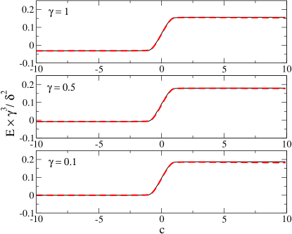
Figure 22: (Color online). Numerical calculation of the error (A80) for different $\gamma$, $\delta$ and $c=\epsilon/|\delta|$. All the curves show that $|E|\times\gamma^{3}/\delta^{2}$ is bounded from above by about $0.2$. They also illustrate that $E$ scales as $\delta^{2}/\gamma^{3}$. Upper panel: $\delta=10^{-3}$ (dashed red line) and $\delta=10^{-5}$ (solid black line); $\gamma=1$ for both curves. Middle panel: $\delta=10^{-4}$ (dashed red line) and $\delta=10^{-6}$ (solid black line); $\gamma=0.5$ for both curves. Bottom panel: $\delta=10^{-5}$ (dashed red line) and $\delta=10^{-7}$ (solid black line); $\gamma=0.1$ for both curves. We keep $|\epsilon|,|\delta|\ll\gamma^{2}$ in these calculations.

Error (A80) is bounded: $|E|<E_{1}+E_{2}$, where

$$E_{1} = \left|\frac{1}{2\pi}\int_{0}^{\pi}dk\ln f_{k}-\frac{1}{2\pi}\int_{0}^{\pi}dk\ln\tilde{f}_{k}\right|$$ (A81)

$$\leq \frac{1}{2\pi}\int_{0}^{\pi}dk\left|\ln f_{k}-\ln\tilde{f}_{k}\right|$$

is due to approximation of $p_{k}$ and $q_{k}$ in (25) by $\tilde{p}_{k}$ and $\tilde{q}_{k}$ (see below) and

$$E_{2}=\left|\frac{1}{2\pi}\int_{\pi}^{\infty}dk\ln\tilde{f}_{k}\right|\leq\frac{1}{2\pi}\int_{\pi}^{\infty}dk\left|\ln\tilde{f}_{k}\right|$$

results from sending the upper integration limit in (26) to infinity. For clarity of our discussion, we repeat the expressions for exact $f_{k}$

$$\ln f_{k} = \frac{1}{2}\ln\left(\frac{1}{2}+\frac{p_{k}}{2\sqrt{p_{k}^{2}+q_{k}^{2}}}\right),$$

$$p_{k} = (1-\cos k)(1-\cos k+2\delta)+\gamma^{2}\sin^{2}k,$$

$$q_{k} = 2\delta\gamma\sin k,$$

and approximated $\tilde{f}_{k}$

$$\ln\tilde{f}_{k} = \frac{1}{2}\ln\left(\frac{1}{2}+\frac{\tilde{p}_{k}}{2\sqrt{\tilde{p}_{k}^{2}+\tilde{q}_{k}^{2}}}\right),$$

$$\tilde{p}_{k} = \gamma^{2}k^{2},\quad\tilde{q}_{k}=2\delta\gamma k.$$

In order to estimate $E_{1}$ we find a function $g_{k}$ such that

$$\left|\ln f_{k}-\ln\tilde{f}_{k}\right|<g_{k}.$$ (A82)

To further simplify our calculations, we assume that $\delta/\gamma^{2}<0.2$: other bounds would give us a slightly different prefactor in the estimation of the magnitude of $E$, but will not change its scaling with $\gamma$ and $\delta$. To derive (A82) we start with inequality:

$$|\ln f_{k}-\ln\tilde{f}_{k}|<0.6\left|f_{k}^{2}/\tilde{f}_{k}^{2}-1\right|,$$ (A83)

which is true when $\left|f_{k}^{2}/\tilde{f}_{k}^{2}-1\right|<0.25$ (the latter will be proved below). We consider

$$\left|f_{k}^{2}/\tilde{f}_{k}^{2}-1\right|=\left|\frac{\frac{p_{k}}{\sqrt{p_{k}^{2}+q_{k}^{2}}}-\frac{\tilde{p}_{k}}{\sqrt{\tilde{p}_{k}^{2}+\tilde{q}_{k}^{2}}}}{1+\frac{\tilde{p}_{k}}{\sqrt{\tilde{p}_{k}^{2}+\tilde{q}_{k}^{2}}}}\right|.$$ (A84)

Two remarks are in order now. First, we will use below that $p_{k},q_{k},\tilde{p}_{k},\tilde{q}_{k}\geq 0$ and $0\leq p_{k}/q_{k}\leq\infty$. Second, we will consider two regions in $k$ separately:

$\bullet$ $k\in[0,2\delta/\gamma]$ or equivalently $0\leq\tilde{p}_{k}/\tilde{q}_{k}<1$.
In this case we estimate (A84) as

$$\left|f_{k}^{2}/\tilde{f}_{k}^{2}-1\right| = \frac{\left|\frac{p_{k}/q_{k}}{\sqrt{1+p_{k}^{2}/q_{k}^{2}}}-\frac{\tilde{p}_{k}/\tilde{q}_{k}}{\sqrt{1+\tilde{p}_{k}^{2}/\tilde{q}_{k}^{2}}}\right|}{1+\frac{\tilde{p}_{k}/\tilde{q}_{k}}{\sqrt{1+\tilde{p}_{k}^{2}/\tilde{q}_{k}^{2}}}}$$

$$\leq \left|\frac{p_{k}/q_{k}}{\sqrt{1+p_{k}^{2}/q_{k}^{2}}}-\frac{\tilde{p}_{k}/\tilde{q}_{k}}{\sqrt{1+\tilde{p}_{k}^{2}/\tilde{q}_{k}^{2}}}\right|$$

$$\leq \left|p_{k}/q_{k}-\tilde{p}_{k}/\tilde{q}_{k}\right|=g_{k}/0.6.$$

Above, in the first step we bounded denominator by $1$ and in the second step we used inequality $\left|x/\sqrt{1+x^{2}}-y/\sqrt{1+y^{2}}\right|\leq\left|x-y\right|$. Subsequent study of $|p_{k}/q_{k}-\tilde{p}_{k}/\tilde{q}_{k}|$ reveals that $\left|f_{k}^{2}/\tilde{f}_{k}^{2}-1\right|<0.25$ when $\delta/\gamma^{2}<0.2$. This in turn validates inequality (A83) in the considered $k$-region. The above estimation provides us also with the expression for $g_{k}$ from (A82): $g_{k}=0.6|p_{k}/q_{k}-\tilde{p}_{k}/\tilde{q}_{k}|$. We integrate it over $k$, and simplify the result getting

$$\frac{1}{2\pi}\int_{0}^{2\delta/\gamma}dk\,g_{k}<0.11~{}\delta^{2}/\gamma^{3}.$$ (A85)

$\bullet$ $k\in[2\delta/\gamma,\pi]$ or equivalently $0\leq\tilde{q}_{k}/\tilde{p}_{k}<1$.
In that case we estimate (A84) as

$$\left|f_{k}^{2}/\tilde{f}_{k}^{2}-1\right| = \frac{\left|\frac{1}{\sqrt{1+q_{k}^{2}/p_{k}^{2}}}-\frac{1}{\sqrt{1+\tilde{q}_{k}^{2}/\tilde{p}_{k}^{2}}}\right|}{1+\frac{1}{\sqrt{1+\tilde{q}_{k}^{2}/\tilde{p}_{k}^{2}}}}$$

$$\leq \frac{1}{1+1/\sqrt{2}}\left|\frac{1}{\sqrt{1+q_{k}^{2}/p_{k}^{2}}}-\frac{1}{\sqrt{1+\tilde{q}_{k}^{2}/\tilde{p}_{k}^{2}}}\right|$$

$$\leq \frac{1}{2+\sqrt{2}}\left|q_{k}^{2}/p_{k}^{2}-\tilde{q}_{k}^{2}/\tilde{p}_{k}^{2}\right|=g_{k}/0.6,$$

where in the first step we bounded denominator by $1+1/\sqrt{2}$ and later we used inequality $\left|1/\sqrt{1+x^{2}}-1/\sqrt{1+y^{2}}\right|\leq\left|x^{2}-y^{2}\right|/2$. A careful study of $\frac{1}{2+\sqrt{2}}\left|q_{k}^{2}/p_{k}^{2}-\tilde{q}_{k}^{2}/\tilde{p}_{k}^{2}\right|$ shows that $\left|f_{k}^{2}/\tilde{f}_{k}^{2}-1\right|<0.25$ when $\delta/\gamma^{2}<0.2$. It validates inequality (A83) in the studied $k$-region. From the above calculation we see that $g_{k}$ from (A82) is equal to $\frac{0.6}{2+\sqrt{2}}\left|q_{k}^{2}/p_{k}^{2}-\tilde{q}_{k}^{2}/\tilde{p}_{k}^{2}\right|$. It can be integrated over $k$ and the obtained result can be simplified to yield

$$\frac{1}{2\pi}\int_{2\delta/\gamma}^{\pi}dk~{}g_{k}<0.25~{}\delta^{2}/\gamma^{3}.$$ (A86)

This concludes our proof of (A83) for $\delta/\gamma^{2}<0.2$.

Combining (A81) with (A82), (A85) and (A86) we obtain

$$E_{1}<0.36~{}\delta^{2}/\gamma^{3}.$$ (A87)

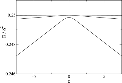
Figure 23: Integration error (A89). The curves from bottom to top correspond to $\delta=10^{-3}$, $10^{-4}$ and $10^{-5}$, respectively. For each $\delta$ we choose $g=0,0.9,1$. The curves for different $g$’s, but the same $\delta$, perfectly collapse onto each other. This plot supports $E\approx 0.25\,\delta^{2}$.

Estimation of $E_{2}$ is straightforward because

$$E_{2}\leq\frac{1}{2\pi}\int_{\pi}^{\infty}dk|\ln\tilde{f}_{k}|=$$ (A88)

$$\frac{|\delta|}{4\pi\gamma}\int_{\pi\gamma/\delta}^{\infty}dl\left|\ln\left(\frac{1}{2}+\frac{1}{2\sqrt{1+4/l^{2}}}\right)\right|<$$

$$\frac{|\delta|}{4\pi\gamma}\int_{\pi\gamma/\delta}^{\infty}\frac{dl}{l^{2}}=\frac{\delta^{2}}{4\pi^{2}\gamma^{2}}<0.03~{}\delta^{2}/\gamma^{3}.$$

Summing up the contributions (A87) and (A88) we find that

$$|E|<0.4\,\delta^{2}/\gamma^{3}$$

when $\epsilon=\delta$ ($c=1$). This is in agreement with Fig. 22, which in fact suggests a stronger bound, and extends our analytical results beyond the $\epsilon=\delta$ case.

Approximations in Sec. III.2. We justify here numerically the ${\cal O}(\delta^{2})$ error in (44). To that end we look at

$$E=\frac{1}{2\pi}\int_{0}^{\pi}dk\ln f_{k}-\left(-2|\delta|A(c)\right),$$ (A89)

where this time $f_{k}$ is given exactly by (11,40,41). The numerical results for various values of parameters are presented in Fig. 23. It shows that the error scales as ${\cal O}(\delta^{2})$ confirming that our approximation correctly captures leading universal contribution to ${\cal F}_{\rm smooth}$. We note also that our numerics suggests that the error, and in principle the exact value of the integral (44), do not depend on $g\in[-1,1]$.

References

- Sachdev (1999) S. Sachdev, Quantum Phase Transitions (Cambridge University Press, Cambridge, U.K., 1999).
- Coldea et al. (2010) R. Coldea, D. A. Tennant, E. M. Wheeler, E. Wawrzynska, D. Prabhakaran, M. Telling, K. Habicht, P. Smeibidl, and K. Kiefer, Science 327, 177 (2010).
- (3) L. E. Sadler, J. M. Higbie, S. R. Leslie, M. Vengalattore and D. M. Stamper-Kurn, Nature (London) 443, 312 (2006).
- (4) M. Greiner, O. Mandel, T. Esslinger, T. W. Hänsch, and I. Bloch, Nature (London) 415, 39 (2002); R. Jördens, N. Strohmaier, K. Günter, H. Moritz, and T. Esslinger, Nature (London) 455, 204 (2008); M. Lewenstein, A. Sanpera, V. Ahufinger, B. Damski, A. Sen(De), and U. Sen, Adv. Phys. 56, 243 (2007).
- Lee et al. (2006) P. A. Lee, N. Nagaosa, and X.-G. Wen, Rev. Mod. Phys. 78, 17 (2006).
- (6) A. Osterloh, L. Amico, G. Falci, and R. Fazio, Nature (London) 416, 608 (2002).
- Zanardi and Paunković (2006) P. Zanardi and N. Paunković, Phys. Rev. E 74, 031123 (2006).
- Gu (2010) S.-J. Gu, Int. J. Mod. Phys. B 24, 4371 (2010).
- Wolf et al. (2006) M. M. Wolf, G. Ortiz, F. Verstraete, and J. I. Cirac, Phys. Rev. Lett. 97, 110403 (2006).
- Campos Venuti and Zanardi (2007) L. Campos Venuti and P. Zanardi, Phys. Rev. Lett. 99, 095701 (2007).
- Schwandt et al. (2009) D. Schwandt, F. Alet, and S. Capponi, Phys. Rev. Lett. 103, 170501 (2009).
- Albuquerque et al. (2010) A. F. Albuquerque, F. Alet, C. Sire, and S. Capponi, Phys. Rev. B 81, 064418 (2010).
- Barankov (2009) R. A. Barankov, ArXiv e-prints (2009), eprint 0910.0255.
- De Grandi et al. (2010a) C. De Grandi, V. Gritsev, and A. Polkovnikov, Phys. Rev. B 81, 012303 (2010a).
- De Grandi et al. (2010b) C. De Grandi, V. Gritsev, and A. Polkovnikov, Phys. Rev. B 81, 224301 (2010b).
- (16) V. Gritsev and A. Polkovnikov, in Understanding in Quantum Phase Transitions edited by L. Carr (Taylor & Francis, Boca Raton, 2010); arXiv:0910.3692.
- Rams and Damski (2011) M. M. Rams and B. Damski, Phys. Rev. Lett. 106, 055701 (2011).
- You et al. (2007) W.-L. You, Y.-W. Li, and S.-J. Gu, Phys. Rev. E 76, 022101 (2007).
- Sirker (2010) J. Sirker, Phys. Rev. Lett. 105, 117203 (2010).
- Zanardi et al. (2007) P. Zanardi, H. T. Quan, X. Wang, and C. P. Sun, Phys. Rev. A 75, 032109 (2007).
- Quan and Cucchietti (2009) H. T. Quan and F. M. Cucchietti, Phys. Rev. E 79, 031101 (2009).
- Cozzini et al. (2007) M. Cozzini, R. Ionicioiu, and P. Zanardi, Phys. Rev. B 76, 104420 (2007).
- Zhou and Barjaktarevič (2008) H. Zhou and J. P. Barjaktarevič, J. Phys. A 41, 412001 (2008).
- Anderson (1967) P. W. Anderson, Phys. Rev. Lett. 18, 1049 (1967).
- Bettelheim et al. (2006) E. Bettelheim, A. G. Abanov, and P. Wiegmann, Phys. Rev. Lett. 97, 246402 (2006).
- Dziarmaga (2010) J. Dziarmaga, Adv. Phys. 59, 1063 (2010).
- Polkovnikov et al. (2011) A. Polkovnikov, K. Sengupta, A. Silva, and M. Vengalattore, Rev. Mod. Phys. 83, 863 (2011).
- Damski et al. (2011) B. Damski, H. T. Quan, and W. H. Zurek, Phys. Rev. A 83, 062104 (2011).
- Vojta (2003) M. Vojta, Rep. Prog. Phys. 66, 2069 (2003).
- (30) J. Zakrzewski and D. Delande, in Proceedings of Let’s Face Chaos Through Nonlinear Dynamics, 7th International Summer School and Conference (AIP, 2008), Vol. 1076, pp. 292-300 (2008).
- Zhou et al. (2008a) H.-Q. Zhou, R. Orús, and G. Vidal, Phys. Rev. Lett. 100, 080601 (2008a).
- Zhou et al. (2008b) H.-Q. Zhou, J.-H. Zhao, and B. Li, J. Phys. A 41, 492002 (2008b).
- Lieb et al. (1961) E. Lieb, T. Schultz, and D. Mattis, Ann. Phys. (N.Y.) 16, 407 (1961).
- Barouch and McCoy (1971) E. Barouch and B. M. McCoy, Phys. Rev. A 3, 786 (1971).
- Bunder and McKenzie (1999) J. E. Bunder and R. H. McKenzie, Phys. Rev. B 60, 344 (1999).
- Damle and Sachdev (1996) K. Damle and S. Sachdev, Phys. Rev. Lett. 76, 4412 (1996).
- Mukherjee et al. (2011) V. Mukherjee, A. Polkovnikov, and A. Dutta, Phys. Rev. B 83, 075118 (2011).
- Dziarmaga (2005) J. Dziarmaga, Phys. Rev. Lett. 95, 245701 (2005).
- (39) We perform least squares linear fitting. The errors that we provide correspond to one standard deviation.
- (40) I. S. Gradshteyn and I. S. Ryzhik, Table of Integrals, Series, and Products, 7th ed. (Academic Press, San Diego, 2007).
- Yang et al. (2008) S. Yang, S.-J. Gu, C.-P. Sun, and H.-Q. Lin, Phys. Rev. A 78, 012304 (2008).
- Deng et al. (2008) S. Deng, G. Ortiz, and L. Viola, Europhysics Letters 84, 67008 (2008).
- Deng et al. (2011) S. Deng, G. Ortiz, and L. Viola, Phys. Rev. B 83, 094304 (2011).
- Damski (2005) B. Damski, Phys. Rev. Lett. 95, 035701 (2005).
- Zurek et al. (2005) W. H. Zurek, U. Dorner, and P. Zoller, Phys. Rev. Lett. 95, 105701 (2005).
- Cincio et al. (2009) L. Cincio, J. Dziarmaga, J. Meisner, and M. M. Rams, Phys. Rev. B 79, 094421 (2009).