Power Allocation Based on SEP Minimization in Two-Hop Decode-and-Forward Relay Networks

Abstract

The problem of optimal power allocation among the relays in a two-hop decode-and-forward cooperative relay network with independent Rayleigh fading channels is considered. It is assumed that only the relays that decode the source message correctly contribute in data transmission. Moreover, only the knowledge of statistical channel state information is available. A new simple closed-form expression for the average symbol error probability is derived. Based on this expression, a new power allocation method that minimizes the average symbol error probability and takes into account the constraints on the total average power of all the relay nodes and maximum instant power of each relay node is developed. The corresponding optimization problem is shown to be a convex problem that can be solved using interior point methods. However, an approximate closed-form solution is obtained and shown to be practically more appealing due to significant complexity reduction. The accuracy of the approximation is discussed. Moreover, the so obtained closed-form solution gives additional insights into the optimal power allocation problem. Simulation results confirm the improved performance of the proposed power allocation scheme as compared to other schemes.

I Introduction

Cooperative relay networks enjoy the advantages of the multiple-input multiple-output (MIMO) systems such as, for example, high data rate and low probability of outage by exploiting the inherent spatial diversity without applying multiple antennas at the nodes. In cooperative relay networks, after receiving the source message, relay nodes process and then retransmit it to the destination. Different cooperation protocols such as decode-and-forward (DF), amplify-and-forward (AF), coded cooperation, and compress-and-forward can be used for processing the message at the relay nodes [1], [2]. The benefits of cooperative relay networks can be further exploited by optimal power allocation among the source and relay nodes. Specifically, based on the knowledge of the channel state information (CSI) at the relays and/or destination, the system performance can be improved by optimally allocating the available power resources among the relays [1]–[3].

Different power allocation schemes have been proposed in the literature [6]–[15]. These schemes differ from each other due to the different considerations on the network topology, assumptions on the available CSI, use of different cooperation protocols for relay nodes, and use of different performance criteria [1]. Most of the existing power allocation methods require the knowledge of instantaneous CSI to enable optimal power distribution [1], [6]–[9]. The application of such methods is practically limited due to the significant amount of feedback needed for transmitting the estimated channel coefficients and/or the power levels of different nodes. This overhead problem becomes even more severe when the rate of change of the channel fading coefficients is fast.

In this paper, we aim at avoiding the overhead problem by considering only statistical CSI which is easy to obtain. Recently, some power allocation methods based on statistical CSI have been proposed[10]–[14]. The optimal power allocation problem among multiple AF relay nodes that minimizes the total power given a required symbol error probability (SEP) at the destination is studied in [11]. The problem of optimal power distribution in a three node DF relay network which aims at minimizing the average SEP is studied in [12]. The authors of [13] study the power allocation problem in a multi-relay DF cooperative network in which the relay nodes cooperate and each relay coherently combines the signals received from previous relays in addition to the signal received from the source to minimize the average SEP. The power allocation problem aiming at minimizing the average SEP in a cooperative network consisting of two DF relay nodes in Nakamgi-$m$ fading channel has been studied in [14]. All of the aforementioned power allocation methods are based on minimizing or bounding the asymptotic approximate average SEP which is valid at high signal-to-noise ratios (SNRs) and is not applicable at low and moderate SNRs.

In our initial conference contribution [15], a power allocation method for multi-relay DF cooperative network with Rayleigh fading channels that minimizes the exact average SEP has been proposed. However, the assumption of correct decoding in relay nodes used in [15] limits its practical applicability. For obtaining a more practically suitable power allocation method, we consider in this paper the case when relay nodes may not be able to decode the source signal correctly. We derive the optimal power allocation in a multi node DF relay network with Rayliegh fading channels in which only relays which have decoded the source message correctly contribute in the data relaying. More specifically, after receiving the source message, only the relays which decode the message correctly retransmit it to the destination. A new exact and simple closed-form expression for average SEP is derived. Then a new power allocation strategy is developed by minimizing the exact average SEP rather than its high SNR approximation under the constraints on the total average power of all relays and maximum powers of individual relays. Only the knowledge of the average channel gains, i.e., the knowledge of the variances of the channel coefficients, is assumed to be available. We show that the corresponding optimization problem is convex and, thus, can be solved using the well established interior point methods. In order to find better insights into the power allocation problem, we derive an approximate closed-form solution to the problem and discuss the accuracy of the approximation used. We also show by simulations that the exact numerical and approximate solutions provide close average SEP performance and that the proposed power allocation scheme outperforms other schemes.

The paper is organized as follows. System model is introduced in Section II. A simple closed-form expression for the average SEP is derived in Section III, while power allocation (exact and approximate) strategies based on SEP minimization are derived in Section IV. Simulation results are given in Section V followed by conclusion. All technical proofs are given in Appendix. This paper is reproducible research [16] and the software needed to generate the simulation results will be made available together with the paper. It can be also requested by the reviewers if needed.

II System Model

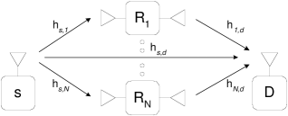
Figure 1: System Model: A single source communicates with a single destination through $N$ relay nodes and a direct path.

Consider a wireless relay network with a single source communicating with a single destination through $N$ relay nodes as it is shown in Fig. 1. The relays are assumed to be half-duplex, that is, the relays either transmit or receive the signal at the same frequency at any given time instant. Therefore, every data transmission from the source to the destination occurs in two phases. In the first phase, the source node transmits its message to the destination and the relay nodes, while in the second phase, relay nodes retransmit the source message to the destination. The channels between the source and the relay nodes, between the relay nodes and the destination, and the direct path are assumed to be flat Rayligh fading and independent from each other. The source and relay nodes use the $M$-phase shift keying (M-PSK) modulation for data transmission where $M$ is the size of the constellation. Relay nodes use DF cooperation protocol for processing the received signal from the source node. The received signal at the destination and the $i$th relay node in the first phase can be expressed, respectively, as

$$y_{s,d} = \sqrt{p_{0}}h_{s,d}x+n_{s,d}$$ (1)

$$y_{s,i} = \sqrt{p_{0}}h_{s,i}x+n_{s,i},\ \ \ \ \ i=1,\ldots,N$$ (2)

where $x$ is the source message of unit power, $p_{0}$ is the transmit power of the source node, $h_{s,d}$ and $h_{s,i}$ denote the channel coefficients between the source and the destination and between the source and the $i$th relay node, respectively, and $n_{s,d}$ and $n_{s,i}$ are the complex additive white Gaussian noises (AWGNs) in the destination and in the $i$th relay, respectively. Since the channel fading is Rayleigh distributed, the channel coefficients are modeled as independent complex Gaussian random variables with zero mean and variances $m_{s,d}$ and $m_{s,i}$, respectively, for the channels between the source and the destination and between the source and the $i$th relay node. The additive noises are zero mean and have variance $N_{0}$.

After decoding the received signal from the source (2), only the relay nodes which have decoded the source message correctly retransmit it to the destination through orthogonal channels using time division multiple access (TDMA) or frequency division multiple access (FDMA). By means of an ideal cyclic redundancy check (CRC) code applied to the transmitted information from the source, relays can determine whether they have decoded the received signal correctly or not [12]. Then the probability that $i$th relay node can decode the received signal correctly conditioned on the instantaneous CSI can be expressed as [17]

$$\alpha_{i}(h_{s,i})=1-\frac{1}{\pi}\int_{0}^{\frac{M-1}{M}\pi}e^{{-\frac{g_{PSK}}{\sin^{2}(\theta)N_{0}}}|h_{s,i}|^{2}p_{0}}\,d\theta$$ (3)

where $g_{PSK}\triangleq\sin^{2}(\pi/M)$.

Let $\boldsymbol{\phi}=(\phi_{1},\phi_{2},\ldots,\phi_{N})^{T}$ denote a vector that indicates whether each relay has decoded the source message correctly or not. Specifically, $\boldsymbol{\phi}(i)=1$, if $i$th relay node decodes the source message correctly, and $\boldsymbol{\phi}(i)=0$, otherwise. Here $(\cdot)^{T}$ stands for the transpose. In the rest of the paper, we refer to the vector $\boldsymbol{\phi}$ as the vector of decoding state at the relay nodes. Since $\boldsymbol{\phi}$ consists of only binary values, there are in total $2^{N}$ different combinations that the vector $\boldsymbol{\phi}$ can take. Moreover, there is a one-to-one correspondence between the binary representation of decimal numbers $k=0,\ldots,2^{N}-1$ and different values that the vector $\boldsymbol{\phi}$ can take. For example, in a cooperative network with two relays, if the relay enumerated as first decodes the source message correctly and the relay enumerated as second decodes it incorrectly, the corresponding decoding state vector is $(1,0)^{T}$ and the corresponding representation in decimal is $1\cdot 2^{1}+0\cdot 2^{0}=2$. For simplicity, we represent hereafter each possible combination of vector $\boldsymbol{\phi}$ by its corresponding decimal number $k$ and denote this combination as $\boldsymbol{\phi}_{k}$. For example, $\boldsymbol{\phi}_{0}$ corresponds to the situation when all relay nodes decode the source message incorrectly.

The received signal from the $i$th relay node which is able to decode the source message correctly, that is, $\boldsymbol{\phi}(i)=1$, at the destination can be modeled as

$$y_{i,d}=\sqrt{p_{i}}h_{i,d}x+n_{i,d}$$ (4)

where $p_{i}$ is the transmitted power of the $i$th relay node, $h_{i,d}$ is the channel coefficient between the $i$th relay node and the destination, and $n_{i,d}$ is the AWGN with zero mean and variance $N_{0}$. The channel coefficient $h_{i,d}$ is modeled as an independent complex Gaussian random variable with zero mean and variance $m_{i,d}$ due to the Rayleigh fading assumption. It is worth stressing that the assumption that the channel coefficients are independent from each other is applicable for relay networks because the distances between different relay nodes are typically large enough. It is assumed that the destination knows perfectly the instantaneous CSI from the relays to the destination and the instantaneous CSI of the direct link. The knowledge of instantaneous CSI for the links between the source and the relay nodes is not needed. Then the maximal ratio combining (MRC) principle can be used at the destination to combine received signals form the source and relay nodes. As a result of MRC, the received SNR at the destination conditioned on the decoding state at the relay nodes, i.e., $\boldsymbol{\phi}_{k}$, can be expressed as

$$\gamma_{D}(\boldsymbol{\phi}_{k})=\gamma_{s}+\sum_{\{i|\boldsymbol{\phi}_{k}(i)=1\}}\gamma_{i}$$ (5)

where $\gamma_{s}\triangleq p_{0}|h_{s,d}|^{2}/N_{0}$ and $\gamma_{i}\triangleq p_{i}|h_{i,d}|^{2}/N_{0}$ are the received SNRs from the source and the $i$th relay node at the destination, respectively. Here $\gamma_{s}$ and $\gamma_{i}$, $i=1,\cdots,N$ are exponential random variables with means $p_{0}m_{s,d}/N_{0}$ and $p_{i}m_{i,d}/N_{0}$, respectively. Moreover, $\gamma_{s}$ and $\gamma_{i}$, $i=1,\cdots,N$ are all statically independent.

III Average SEP

For the considered case when the data transmission is performed using the M-PSK modulation, the SEP of the signal at the destination conditioned on the channel states $CS=\{h_{s,d},h_{s,i},h_{i,d}\}$ and the decoding state at the relay nodes $\boldsymbol{\phi}_{k}$ can be written as [17]

$$P_{e}\{CS,\boldsymbol{\phi}_{k}\}\!\!\!\!\! = \!\!\!\!\!\frac{1}{\pi}\int_{0}^{\frac{M-1}{M}\pi}e^{-\frac{g_{PSK}}{\sin^{2}(\theta)}\gamma_{D}(\boldsymbol{\phi}_{k})}\,d\theta.$$ (6)

Using the total probability rule, the SEP conditioned on the channel states can be expressed as

$$P_{e}\{CS\}=\sum_{k=0}^{2^{N}-1}P_{r}\{\boldsymbol{\phi}_{k}\}P_{e}\{CS,\boldsymbol{\phi}_{k}\}$$ (7)

where $P_{r}\{\boldsymbol{\phi}_{k}\}$ is the probability of the decoding state $\boldsymbol{\phi}_{k}$ that can be calculated as

$$P_{r}\{{\boldsymbol{\phi}}_{k}\}=\prod_{\{i|{\boldsymbol{\phi}}_{k}(i)=1\}}\alpha_{i}\cdot\prod_{\{i|{\boldsymbol{\phi}}_{k}(i)=0\}}(1-\alpha_{i})$$ (8)

where $\alpha_{i}$ is the probability of correct decoding in $i$th relay node (3). Note that for obtaining (8), the independency of the AWGNs at the relay nodes has been exploited.

The average SEP can be obtained by averaging (7) over $h_{s,d}$, $h_{s,i}$, $i=1,\cdots,N$, and $h_{i,d}$, $i=1,\cdots,N$ and using the fact that $P_{r}\{\boldsymbol{\phi}_{k}\}$ is statistically independent from $P_{e}\{CS,\boldsymbol{\phi}_{k}\}$. The latter follows from the statistical independence between the channel coefficients and the fact that $P_{r}\{\boldsymbol{\phi}_{k}\}$ depends only on $\{h_{s,i}\}_{i=1}^{N}$ and $P_{e}\{CS,\boldsymbol{\phi}_{k}\}$ depends only on $\{h_{i,d}\}_{i=1}^{N}$ and $h_{s,d}$. Then the average SEP can be expressed as

$$P_{e}\!=\!\frac{1}{\pi}\sum_{k=0}^{2^{N}-1}E\left\{P_{r}\{\boldsymbol{\phi}_{k}\}\right\}E\left\{\int_{0}^{\frac{M-1}{M}\pi}\!e^{-\frac{g_{PSK}}{\sin^{2}(\theta)}\gamma_{D}(\boldsymbol{\phi}_{k})}\,d\theta\right\}$$ (9)

where $E\{\cdot\}$ denotes the expectation operation.

The second expectation in (9) can be computed as

$$\!\!\!\!\!E\left\{\int_{0}^{\frac{M-1}{M}\pi}e^{-\frac{g_{PSK}}{\sin^{2}(\theta)}\gamma_{D}(\boldsymbol{\phi}_{k})}\,d\theta\right\}$$ (10)

$$= \!\!\!\!\!\int_{0}^{\frac{M-1}{M}\pi}\!E\left\{e^{-\frac{g_{PSK}}{\sin^{2}(\theta)N_{0}}\left(\sum\limits_{\{i|\boldsymbol{\phi}_{k}(i)=1\}}p_{i}|h_{i,d}|^{2}+p_{0}|h_{s,d}|^{2}\right)}\right\}\,d\theta$$

$$= \!\!\!\!\!\int_{0}^{\frac{M-1}{M}\pi}\prod_{\{i|\boldsymbol{\phi}_{k}(i)=1\}\cup\{i=0\}}\!\frac{\sin^{2}(\theta)}{\sin^{2}(\theta)\!+\!b_{i}p_{i}}\,d\theta$$

where $b_{i}\triangleq g_{PSK}m_{i,d}/N_{0}$, $i=1,\ldots,N$ and $b_{0}\triangleq g_{PSK}m_{s,d}/N_{0}$. Similarly, the first expectation in (9) can be computed as

$$E\left\{Pr\{\boldsymbol{\phi}_{k}\}\right\}\!\! = \!\!E\left\{\prod_{\{i|\boldsymbol{\phi}_{k}(i)=1\}}\!\alpha_{i}\cdot\prod_{\{i|\boldsymbol{\Phi}_{k}(i)=0\}}(1-\alpha_{i})\right\}$$ (11)

$$= \!\!\prod_{\{i|\boldsymbol{\Phi}_{k}(i)=1\}}\beta_{i}\cdot\prod_{\{i|\boldsymbol{\Phi}_{k}(i)=0\}}(1-\beta_{i})$$

where

$$\beta_{i}\!\! = \!\!E\left\{1-\frac{1}{\pi}\int_{0}^{\frac{M-1}{M}\pi}e^{{-\frac{g_{PSK}}{\sin^{2}(\theta)N_{0}}}|h_{s,i}|^{2}p_{0}}\,d\theta\right\}$$ (12)

$$= \!\!1-\frac{1}{\pi}\int_{0}^{\frac{M-1}{M}\pi}\frac{\sin^{2}(\theta)}{\sin^{2}(\theta)+c_{i}p_{0}}\,d\theta$$

and $c_{i}\triangleq g_{PSK}m_{s,i}/{N_{0}}$, $i=1,\ldots,N$.

Substituting (10) and (11) in (9), the average SEP can be equivalently expressed as

$$P_{e}\!\! = \!\!\frac{1}{\pi}\sum_{k=0}^{2^{N}-1}\left(\prod_{\{i|\boldsymbol{\phi}_{k}(i)=1\}}\beta_{i}\cdot\prod_{\{i|\boldsymbol{\phi}_{k}(i)=0\}}(1-\beta_{i})\right.$$ (13)

$$\times \!\!\left.\int_{0}^{\frac{M-1}{M}\pi}\!\!\!\prod_{\{i|\boldsymbol{\phi}_{k}(i)=1\}\cup\{i=0\}}\frac{\sin^{2}(\theta)}{\sin^{2}(\theta)+b_{i}p_{i}}\,d\theta\right).$$

Setting $\beta_{0}=1$ for notation simplicity, the average SEP expression in (13) can be simplified as

$$P_{e}\!\! = \!\!\frac{1}{\pi}\sum_{k=0}^{2^{N}-1}\left(\prod_{\{i|\boldsymbol{\phi}_{k}(i)=0\}}(1-\beta_{i})\prod_{\{i|\boldsymbol{\phi}_{k}(i)=1\}\cup\{i=0\}}\beta_{i}\right.$$

$$\times \!\!\left.\int_{0}^{\frac{M-1}{M}\pi}\!\!\!\prod_{\{i|\boldsymbol{\Phi}_{k}(i)=1\}\cup\{i=0\}}\frac{\sin^{2}(\theta)}{\sin^{2}(\theta)+b_{i}p_{i}}\,d\theta\right)$$

$$= \!\!\frac{1}{\pi}\int_{0}^{\frac{M-1}{M}\pi}\left(\sum_{k=0}^{2^{N}-1}\prod_{\{i|\boldsymbol{\phi}_{k}(i)=0\}}(1-\beta_{i})\right.$$

$$\times \!\!\left.\prod_{\{i|\boldsymbol{\phi}_{k}(i)=1\}\cup\{i=0\}}\beta_{i}\cdot\frac{\sin^{2}(\theta)}{\sin^{2}(\theta)+b_{i}p_{i}}\,d\theta\right).$$ (15)

Finally, the expression (15) can be further simplified as

$$P_{e}=\frac{1}{\pi}\int_{0}^{\frac{M-1}{M}\pi}\prod_{i=0}^{N}\left((1-\beta_{i})\!+\!\frac{\beta_{i}\sin^{2}(\theta)}{\sin^{2}(\theta)+b_{i}p_{i}}\right)\,d\theta.$$ (16)

To verify the latter result, note that (15) can be obtained by simply expanding (16). Moreover, after finding the integral in (12), $\beta_{i}$, $i=1,\ldots,N$ can be expressed as

$$\beta_{i}\!\! = \!\!1-\!\sqrt{\frac{c_{i}p_{0}}{c_{i}p_{0}\!+\!1}}\!{\left(\!\frac{\tan^{-1}\left(\!\cot\left(\!\frac{M-1}{M}\pi\right)\sqrt{\frac{c_{i}p_{0}}{c_{i}p_{0}\!+\!1}}\right)}{\pi}\!-\!\frac{1}{2}\!\right)}$$ (17)

$$- \!\!\left(\frac{1}{2}\!-\!\frac{\tan^{-1}\left(\cot\left(\frac{M-1}{M}\pi\right)\right)}{\pi}\right),\;i=1,\ldots,N.$$

Here $\beta_{i}$ has a meaning of statistical average of the correct decoding probability in the $i$th relay node (3) with respect to the channel coefficients. It is worth noting that the average SEP expression (16) is used later for finding the optimal power distribution among the relay nodes.

Using partial fraction decomposition, it is possible to further simplify (16) and find a closed-form expression for the average SEP. It is worth noting that for simplicity and because of space limitations, we hereafter assume that $b_{i}\neq b_{j}$, $i\neq j$, $i,j=0,\ldots,N$. However, if the condition $b_{i}\neq b_{j}$, $i\neq j$, $i,j=0,\ldots,N$ does not hold, the following average SEP derivation approach remains unchanged, while the only change is the need of using another form of the partial fraction decomposition. Thus, it is straightforward to derive closed-form expression for the average SEP in the case when $b_{i}\neq b_{j}$, $i\neq j$, $i,j=0,\ldots,N$ does not hold by using the same steps as we show next.

Toward this end, we first rewrite the integral inside (III), denoted hereafter as $I$, by changing the variable as

$$\!\!\!\!\!I\!\! = \!\!\!\!\!\int_{0}^{\frac{M-1}{M}\pi}\prod_{\{i|\boldsymbol{\phi}_{k}(i)=1\}\cup\{i=0\}}\frac{\sin^{2}(\theta)}{\sin^{2}(\theta)+b_{i}p_{i}}\,d\theta$$

$$= \!\!\!\!\!\int_{{\rm cot}\left(\frac{M-1}{M}\pi\right)}^{\infty}\!\frac{1}{1\!+\!x^{2}}\!\!\prod_{\{i|\boldsymbol{\phi}_{k}(i)=1\}\cup\{i=0\}}\!\!\!\frac{1}{(1\!+\!b_{i}p_{i})\!+\!b_{i}p_{i}x^{2}}\,dx.$$

Then applying the partial fraction technique to the right-hand side of (LABEL:EQ2) and using the fact that $b_{i}\neq b_{j}$, $i\neq j$, $i,j=0,\ldots,N$, we obtain

$$I\!\! = \!\!\int_{{\rm cot}\left(\frac{M-1}{M}\pi\right)}^{\infty}\frac{1}{1+x^{2}}\!$$

$$- \!\!\!\!\!\!\sum_{\{i|\boldsymbol{\phi}_{k}(i)=1\}\cup\{i=0\}}\!\!\!\!\!\frac{\prod_{(\{j|\boldsymbol{\phi}_{k}(j)=1\}\cup\{j=0\})-\{j\neq i\}}\frac{1}{1\!-\!\frac{b_{j}p_{j}}{b_{i}p_{i}}}}{(1\!+\!\frac{1}{b_{i}p_{i}})+x^{2}}\,dx.$$

The integral in (LABEL:inint) is the summation of the terms that all have the form of $1/(a+x^{2}),\ a>0$. By using the fact that $\int 1/(a+x^{2})dx=1/\sqrt{a}\tan^{-1}(x/\sqrt{a}),\ a>0$, (LABEL:inint) can be calculated as

$$I\!\! = \!\!\!\!\!\!\!\!\!\sum_{\{\!i|\boldsymbol{\phi}_{k}(i)=1\}\cup\{\!i=0\}}\!\!\!\Bigg{(}\!\!{\Bigg{(}{\tan^{-1}\!\!\left(\!\cot\left(\!\frac{M\!-\!1}{M}\pi\!\!\right)\!\!\sqrt{\frac{b_{i}p_{i}}{b_{i}p_{i}\!+\!1}}\right)}\!-\!\frac{\pi}{2}\!\Bigg{)}}$$ (20)

$$\times \!\!\sqrt{\frac{b_{i}p_{i}}{b_{i}p_{i}\!+\!1}}\prod_{(\{j|\boldsymbol{\phi}_{k}(j)=1\}\cup\{j=0\})-\{j\neq i\}}\frac{1}{1-\frac{b_{j}p_{j}}{b_{i}p_{i}}}\Bigg{)}$$

$$+ \!\!\left(\frac{\pi}{2}-{\tan^{-1}(\cot(\frac{M-1}{M}\pi))}\right)$$

Substituting the so obtained expression (20) in (III) and also expanding the resulted expression, the average SEP can be equivalently expressed as

$$P_{e}\!\!\! = \!\!\!\sum_{k=0}^{2^{N}-1}\!\prod_{\{i|\phi_{k}(i)=1\}\cup\{i=0\}}\!\!\!\!\beta_{i}\cdot\prod_{\{i|\phi_{k}(i)=0\}}^{N}(1-\beta_{i})$$ (21)

$$\times \!\!\!\sum_{\{\!i|\phi_{k}(i)=1\!\}\cup\{\!i=0\}}\!\Bigg{(}\!\!{\Bigg{(}\frac{\tan^{-1}(\cot(\!\frac{M-1}{M}\pi)\sqrt{\frac{b_{i}p_{i}}{b_{i}p_{i}\!+\!1}})}{\pi}\!-\!\frac{1}{2}\Bigg{)}}$$

$$\times \!\!\!\sqrt{\frac{b_{i}p_{i}}{b_{i}p_{i}\!+\!1}}\prod_{(\{\!j|\boldsymbol{\phi}_{k}(j)=1\!\}\cup\{\!j=0\})-\{\!j\neq i\!\}}\frac{1}{1\!-\!\frac{b_{j}p_{j}}{b_{i}p_{i}}}\Bigg{)}$$

$$+ \!\!\!\sum_{k=0}^{2^{N}-1}\!\!\prod_{\{\!i|\phi_{k}(i)=1\!\}\cup\{\!i=0\!\}}\beta_{i}\times\prod_{\{i|\phi_{k}(i)=0\}}^{N}(1-\beta_{i})$$

$$\times \!\!\!\left(\frac{1}{2}-\frac{\tan^{-1}\left(\cot\left(\frac{M-1}{M}\pi\right)\right)}{\pi}\right).$$

Moreover, we can modify the first term of (21) by taking the product $\prod_{\{i|\phi_{k}(i)=1\}\cup\{i=0\}}\beta_{i}$ into the summation part of that term and expanding the product such that $\beta_{i}$ is multiplied by the corresponding term in the summation and also modify the second term of (21) by using the following equality which is easy to prove

$$\sum_{k=0}^{2^{N}-1}\!\!\prod_{\{\!i|\phi_{k}(i)=1\!\}\cup\{\!i=0\!\}}\beta_{i}\cdot\prod_{\{i|\phi_{k}(i)=0\}}^{N}(1-\beta_{i})=1.$$ (22)

By doing so, the average SEP can be rewritten as

$$P_{e}\!\!\! = \!\!\!\sum_{k=0}^{2^{N}-1}\!\prod_{\{i|\Phi_{k}(i)\!=\!0\}}(1\!-\!\beta_{i})$$ (23)

$$\times \!\!\!\sum_{\{\!i|\phi_{k}(i)\!=\!1\!\}\cup\{\!i=0\}}\!\Bigg{(}\!{\beta_{i}\Bigg{(}\frac{\tan^{-1}(\cot(\!\frac{M-1}{M}\pi)\sqrt{\frac{b_{i}p_{i}}{b_{i}p_{i}\!+\!1}})}{\pi}\!-\!\frac{1}{2}\Bigg{)}}$$

$$\times \!\!\!\sqrt{\frac{b_{i}p_{i}}{b_{i}p_{i}\!+\!1}}\prod_{(\{\!j|\boldsymbol{\Phi}_{k}(j)\!=\!1\!\}\cup\{\!j=0\!\})-\{\!j\neq i\!\}}\frac{\beta_{j}}{1\!-\!\frac{b_{j}p_{j}}{b_{i}p_{i}}}\Bigg{)}$$

$$+ \!\!\!\left(\frac{1}{2}\!-\!\frac{\tan^{-1}\left(\cot\left(\frac{M-1}{M}\pi\right)\right)}{\pi}\right).$$

Finally, after rearranging and factoring out the terms, we can obtain the following closed form expression for the average SEP

$$P_{e}\!\!\! = \!\!\!\!\sum_{i=0}^{N}\!\Bigg{(}\!{\beta_{i}\Bigg{(}\frac{\tan^{-1}(\cot(\!\frac{M-1}{M}\pi)\sqrt{\frac{b_{i}p_{i}}{b_{i}p_{i}\!+\!1}})}{\pi}\!-\!\frac{1}{2}\Bigg{)}}\sqrt{\frac{b_{i}p_{i}}{b_{i}p_{i}\!+\!1}}$$ (24)

$$\times \!\!\!\prod_{\{\!j|j=0,\ldots,N\}-\{\!j\neq i\!\}}\left(\frac{\beta_{j}}{1\!-\!\frac{b_{j}p_{j}}{b_{i}p_{i}}}\!+\!(1\!-\!\beta_{j})\right)\Bigg{)}$$

$$+ \!\!\!\left(\frac{1}{2}\!-\!\frac{\tan^{-1}\left(\cot\left(\frac{M-1}{M}\pi\right)\right)}{\pi}\right).$$

Note that (23) can be obtained by simply expanding (24). It is interesting to mention that if we consider similar conditions as in [15], in which all relays are capable of decoding the source message correctly, i.e., $\beta_{i}=1,i=1,\ldots,N$, and also there is no direct link between source and destination, i.e., $b_{0}=0$, the closed-form average SEP (24) simplifies to the one that was obtained in [15]. The closed-form expression (24) is simple and does not include any other functions rather than basic analytic functions.

IV Power allocation

In this section, we address in details the problem of optimal power allocation among the relay nodes such that the average SEP is minimized. Only statistical information on the channel states is used. Moreover, we assume that the power of the source node $p_{0}$ is fixed and, in turn, the average probabilities of the correct decoding of the relays, i.e., $\beta_{i}$, $i=1,\ldots,N$, are also fixed. The relevant figure of merit for the performance of relay network is then the average SEP that is derived above in closed form. It enables us to apply power allocation also in the case when the rate of change of channel fading is high. Since only statistical CSI is available and relay nodes retransmit only if they decode the source message correctly, the averaged power of the relay nodes over CSI and probability of correct decoding need to be considered. It is easy to see that the average power used by the $i$th relay node equals $\beta_{i}p_{i}$. Indeed, since $\beta_{i}$ is the statistical average of the probability of correct decoding in the $i$th relay node, the transmitted power of the $i$th relay node $p_{i}$ weighted by $\beta_{i}$ gives average power used by the $i$th relay node during a single transmission.

In the following, we develop a power allocation strategy by minimizing the average SEP (16), while satisfying the constraint on the total average power used in relay nodes $p_{R}$ and the constraints on maximum instantaneous powers per every relay $p_{i}^{max}$, $i=1,\ldots,N$. With the knowledge of the average channel gains $m_{s,i}={E}\{|h_{s,i}|^{2}\}$, $m_{i,d}={E}\{|h_{i,d}|^{2}\}$, $m_{s,d}={E}\{|h_{s,d}|^{2}\}$, and specifications on $p_{R}$, $p_{i}^{max}$, $i=1,\ldots,N$, and $p_{0}$, the power allocation problem can be formulated as

$$\min_{\mathbf{p}}\ P_{e}(\mathbf{p})$$ (25)

$${\rm s.t.}\quad\sum_{i=1}^{N}\beta_{i}{p_{i}}=p_{R}$$ (26)

$$\qquad\;0\leq p_{i}\leq p_{i}^{max},i=1,\ldots,N.$$ (27)

where $P_{e}(\mathbf{p})$ is the average SEP (16) written as a function of powers at the relay nodes $\mathbf{p}=(p_{1},\ldots,p_{N})^{T}$. For notation simplicity, we use hereafter the following equation for the average SEP in (16)

$$P_{e}(\mathbf{p})=\frac{1}{\pi}\int_{0}^{\frac{M-1}{M}\pi}g(\theta,\mathbf{p})\,d\theta$$ (28)

where

$$g(\theta,\mathbf{p})\triangleq\prod_{i=0}^{N}\bigg{(}(1-\beta_{i})+\beta_{i}\frac{\sin^{2}(\theta)}{\sin^{2}(\theta)+b_{i}p_{i}}\bigg{)}.$$ (29)

Note that the optimization problem (25)–(27) is infeasible if $\sum_{i=1}^{N}\beta_{i}p_{i}^{max}<p_{R}$ and it has the trivial solution, that is, $p_{i}=p_{i}^{max}$, if $\sum_{i=1}^{N}\beta_{i}p_{i}^{max}=p_{R}$. Thus, it is assumed that $\sum_{i=1}^{N}\beta_{i}p_{i}^{max}>p_{R}$. The following theorem about convexity of the optimization problem (25)–(27) is in order.

Theorem 1: The optimization problem (25)–(27) is convex.

See the proof in Appendix A.

Although this problem does not have a simple closed-form solution, an accurate approximate closed-form solution can be found as it is shown in the rest of the paper. A numerical algorithm for finding the exact solution of the optimization problem (25)–(27) based on the interior-point methods is summarized in Appendix B. Despite the higher complexity of the numerical method as compared to the approximate closed-form solution, numerical method can provide an exact solution, which can be used as a benchmark to evaluate the accuracy of the approximate solution.

IV-A Approximate Closed-Form Solution

The optimization problem (25)–(27) is strictly feasible because $\sum_{i=1}^{N}\beta_{i}p_{i}^{max}>p_{R}$ as it has been assumed earlier. Thus, the Slater’s condition holds and since the problem is convex, the Karush-Kuhn-Tucker (KKT) conditions are the necessary and sufficient optimality conditions [18]. Indeed, since $\sum_{i=1}^{N}\beta_{i}p_{i}^{max}>p_{R}$, then $p_{i}=p_{i}^{max}p_{R}/(\sum_{i=1}^{N}\beta_{i}p_{i}^{max})$ is a strictly feasible point for the optimization problem (25)–(27).

Let us introduce the Lagrangian

$$L(\mathbf{p},\boldsymbol{\lambda},\boldsymbol{\gamma},\nu)\!\!\! = \!\!\!\!\!\frac{1}{\pi}\!\int_{0}^{\frac{M\!-\!1}{M}\pi}g(\theta,\mathbf{p})\,d\theta\!-\!\sum_{i=1}^{N}\lambda_{i}p_{i}$$

$$+\!\!\!\!\!\! \!\!\!\!\!\!\!\!\!\sum_{i=1}^{N}\gamma_{i}(p_{i}\!-\!p_{i}^{max})\!+\!\nu\!\!\left(\sum_{i=1}^{N}{\beta_{i}p_{i}}\!-\!p_{R}\!\!\right)$$ (30)

where ${\boldsymbol{\lambda}}\triangleq(\lambda_{1},\cdots,\lambda_{N})^{T}$ and $\boldsymbol{\gamma}\triangleq(\gamma_{1},\cdots,\gamma_{N})^{T}$ are $N\times 1$ vectors of non-negative Lagrange multipliers associated with the inequality constraints $p_{i}\geq 0$, $i=1,\cdots,N$ and $p_{i}\leq p_{i}^{max}$, $i=1,\cdots,N$, respectively, and $\nu$ is the Lagrange multiplier associated with the equality constraint $\sum_{i=1}^{N}{p_{i}}=p_{R}$. Then the KKT conditions can be obtained as

$$\lambda_{i}\geq 0,\ \ \ \ \ \gamma_{i}\geq 0,\;\ \ \ \ \;i=1,\cdots,N$$ (31)

$$\lambda_{i}p_{i}=0,\quad\gamma_{i}(p_{i}-p_{i}^{max})=0,\;i=1,\cdots,N$$ (32)

$$\frac{1}{\pi}\!\!\int_{0}^{\frac{M-1}{M}\pi}\!\!\!\!\!\!\!\!\!\!\!\frac{-\beta_{i}b_{i}\sin^{2}(\theta)g(\theta,\mathbf{p})}{\sin^{4}(\theta)\!+\!(2-\beta_{i})b_{i}p_{i}\sin^{2}(\theta)\!+\!(1-\beta_{i})b_{i}^{2}p_{i}^{2}}\,d\theta$$

$$\qquad+\nu\beta_{i}-\lambda_{i}+\gamma_{i}\!=\!0,\qquad i=1,\cdots,N$$ (33)

$$0\leq p_{i}\leq p_{i}^{max},\ \ \ \ \ i=1,\cdots,N$$ (34)

$$\sum_{i=1}^{N}{\beta_{i}p_{i}}=p_{R}.$$ (35)

Although the exact optimal solution of the problem (25)–(27) can be found through solving the system (31)–(35) numerically or as it is summarized in Appendix B by solving the original problem directly, a near optimum closed-form solution for the system (31)–(35), and thus, optimization problem (25)–(27) can be found by approximating the gradient of the Lagrangian, that is, the left hand side of (33). Specifically, it can be verified that for fixed $p_{i}$, $i=1,\ldots,N$ the function $g(\theta,\mathbf{p})$ is strictly increasing/decreasing with respect to $\theta$ in the intervals $(0,{\pi}/{2})$ and $({\pi}/{2},{(M-1)\pi}/{M})$, correspondingly. Under the condition that the number of relays is large enough, the slope of the increment and decrement in the aforementioned intervals is high and the Chebyshev-type approximation on the conditions (33) is highly accurate. This approximation of the conditions (33) is of the form

$$-\frac{\beta_{i}b_{i}}{\pi(1\!+\!(2-\beta_{i})b_{i}p_{i}\!+\!(1-\beta_{i})b_{i}^{2}p_{i}^{2})}$$

$$\times\int^{\frac{M-1}{M}\pi}_{0}\!\!\!\!\!g(\theta,\mathbf{p})d\theta+\beta_{i}\nu-{\lambda}_{i}+{\gamma}_{i}=0,$$ (36)

$$\!\!\!\!\!\!\!\!\!\!\!\!\!\!\!\!\!\!\!\!\!\!\!\!\!\!\!\!i=1,\cdots,N$$

where the fact that $\sin^{2}(\pi/2)=1$ is used in the ratio

$$\frac{-\beta_{i}b_{i}\sin^{2}(\theta)}{\sin^{4}(\theta)\!+\!(2-\beta_{i})b_{i}p_{i}\sin^{2}(\theta)\!+\!(1-\beta_{i})b_{i}^{2}p_{i}^{2}}$$ (37)

By rearranging the denominator of (37), substituting the approximation (36) in (33), dividing the equations (31)–(33) by the positive quantity $\int_{0}^{\frac{M-1}{M}\pi}g(\theta,\mathbf{p})\,d\theta$, and also multiplying these equations by $\pi$, we obtain

$$\lambda_{i}^{\prime}\geq 0,\ \ \ \ \ \gamma_{i}^{\prime}\geq 0,\;\ \ \ \ \;i=1,\cdots,N$$ (38)

$$\lambda_{i}^{\prime}p_{i}=0,\quad\gamma_{i}^{\prime}(p_{i}-p_{i}^{max})=0,\;i=1,\cdots,N$$ (39)

$$-\frac{\beta_{i}b_{i}}{\beta_{i}(1\!+\!b_{i}p_{i})\!+\!(1\!-\!\beta_{i})(1\!+\!b_{i}p_{i})^{2}}\!+\!\beta_{i}{\nu}^{\prime}\!-\!\lambda_{i}^{\prime}\!+\!{{\gamma}_{i}}^{\prime}\!\!=\!0$$

$$\qquad\qquad\qquad\qquad\qquad\qquad\qquad i=1,\cdots,N$$ (40)

$$0\leq p_{i}\leq p_{i}^{max},\ \ \ \ \ i=1,\cdots,N$$ (41)

$$\sum_{i=1}^{N}{\beta_{i}p_{i}}=p_{R}.$$ (42)

where ${\nu}^{\prime}\triangleq\nu\pi/\int_{0}^{\frac{M-1}{M}\pi}g(\theta)\,d\theta$, ${\gamma}_{i}^{\prime}\triangleq{\gamma}_{i}\pi/\int_{0}^{\frac{M-1}{M}\pi}g(\theta)\,d\theta$, and  ${\lambda}_{i}^{\prime}$ $\triangleq{\lambda}_{i}\pi/\int_{0}^{\frac{M-1}{M}\pi}g(\theta)\,d\theta$, $i=1,\cdots,N$. It is possible to eliminate $\lambda_{i}^{\prime}$ from the set of equations (38)–(42) in order to find a simpler set of smaller number of equations. By doing so, the approximate KKT conditions can be equivalently rewritten as

$${{\gamma}_{i}}^{\prime}\geq 0,\quad i=1,\cdots,N$$ (43)

$${{\gamma}_{i}}^{\prime}\left(p_{i}-{p_{i}}^{max}\right)=0,\qquad i=1,\cdots,N$$ (44)

$$p_{i}\left(\beta_{i}{\nu}^{\prime}\!+\!{{\gamma}_{i}}^{\prime}-\frac{\beta_{i}b_{i}}{\beta_{i}(1\!+\!b_{i}p_{i})\!+\!(1\!-\!\beta_{i})(1\!+\!b_{i}p_{i})^{2}}\!\right)\!=\!0,\;$$

$$\qquad\qquad\qquad\qquad\qquad\qquad\quad i=1,\cdots,N$$ (45)

$$\frac{\beta_{i}b_{i}}{\beta_{i}(1\!+\!b_{i}p_{i})\!+\!(1\!-\!\beta_{i})(1\!+\!b_{i}p_{i})^{2}}\!\leq\beta_{i}{\nu}^{\prime}+{{\gamma}_{i}}^{\prime},$$

$$\qquad\qquad\qquad\quad\qquad\qquad\qquad i=1,\cdots,N$$ (46)

$${0\leq\ p}_{i}\ \leq{p_{i}}^{max},\quad i=1,\cdots,N$$ (47)

$$\sum^{N}_{i=1}\beta_{i}{p_{i}}=p_{R}$$ (48)

Note that (40) is rewritten as (IV-A) since $\lambda_{i}$ or, equivalently, $\lambda_{i}^{\prime}$ is positive. Moreover, (IV-A) is obtained by solving (40) with respect to $\lambda_{i}^{\prime}$ and then substituting the result in $\lambda_{i}^{\prime}p_{i}=0$. The following result gives a closed-form solution for the system (43)–(48), and thus, it also gives an approximate solution for the power allocation optimization problem (25)–(27).

Theorem 2: For a set of DF relays, the approximate power allocation $\{p_{1}\ ,\dots,\ p_{N}\}$, i.e., the approximate solution of the optimization problem (25)-(27), is

$$p_{i}=\left(\frac{-\beta_{i}+\sqrt{\beta_{i}^{2}+4(1-\beta_{i})b_{i}/{\nu}^{\prime}}}{2b_{i}(1-\beta_{i})}-\frac{1}{b_{i}}\right)_{0}^{p_{i}^{max}}$$ (49)

where ${\nu}^{\prime}$ is determined so that $\sum_{i=1}^{N}\beta_{i}p_{i}=p_{R}$.

See the proof in Appendix C.

It is interesting to mention that the power allocation scheme of [15] is a special case of the power allocation method given by (49) when ${\beta_{i}\rightarrow 1}$. Indeed, it can be checked that for ${\beta_{i}\rightarrow 1}$, we have

$$p_{i}\!\!\! = \!\!\!\left(\lim_{\beta_{i}\rightarrow 1}\frac{-\!\beta_{i}\!+\!\sqrt{\beta_{i}^{2}\!+\!4(1\!-\!\beta_{i})b_{i}/{\nu}^{\prime}}}{2b_{i}(1\!-\!\beta_{i})}\!-\!\frac{1}{b_{i}}\right)_{0}^{p_{i}^{max}}$$ (50)

$$= \!\!\!\left(\frac{1}{\nu^{\prime}}-\frac{1}{b_{i}}\right)_{0}^{p_{i}^{max}}$$

This special case shows that the total power should be distributed only among relays from a selected set and the relays with ‘better’ channel conditions use bigger portion of the total power. Note that this solution can be viewed as a form of water-filling solution and has similar complexity. However, the solution (49) is not interpretable only by the means of water-filling, and the optimal power allocation among the relays and relay admission depend on the average probability of correct decoding by relay nodes and also on the corresponding average channel gain-to-noise ratios for admitted relays.

V Simulation results

We consider a cooperative relay network consisting of a source-destination pair and $N=5$ DF relay nodes. In the first phase, source transmits its message to the destination and the relay nodes, while in the second phase, only the relay nodes, which decoded the source message correctly, retransmit it to the destination. All the nodes use QPSK modulation for data transmission and noise power is assumed to be equal to $1$. Relays are assumed to be located on a line of unit length connecting the source and the destination nodes. Positions of the relay nodes with respect to the source node are then randomly selected according to the uniform distribution and are $\{0.0117,0.1365,0.2844,0.4692,0.8938\}$. All the channel coefficients are modeled as zero mean complex Gaussian random variables. The variance of the channel coefficient between $p$th and $q$th nodes is $1/d_{p,q}^{\nu}$ where $d_{p,q}$ is the distance between the nodes and $2\leq\nu\leq 6$ is the path-loss parameter which is assumed to be equal to $3$ throughout our simulations.

V-A Closed-Form SEP

We first aim at comparing the closed form SEP expression (24) with the SEP obtained through Monte-Carlo simulations and demonstrating their equivalence. The source node transmits its message to the destination node through only the relay nodes $1,3,5$ or all relay nodes $1,2,3,4,5$. The total power is equally divided among the source and the relay nodes. Fig. 1 shows the average SEP corresponding to the closed-form expression (24) and the SEP found by Monte-Carlo simulations with each point obtained by averaging over $10^{8}$ independent runs. The corresponding SEPs are shown versus the total power. Fig. 1 confirms the fact that the closed-form expression (24) results in the same average SEP as the one obtained through numerical simulations. The closed-form-based SEP and the SEP obtained through numerical simulations coincide in both scenarios considered with 3 and 5 relay nodes.

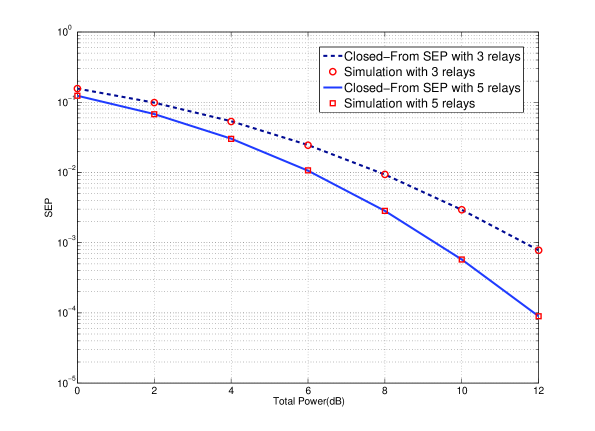
Figure 2: Average SEP obtained through Monte-Carlo simulations and by using the closed form SEP expression (24).

V-B Accuracy of the Approximate Closed-Form Solution

In this simulation example, we study the accuracy of the proposed approximate power allocation method (see Theorem 2) by comparing its performance to that of the optimal SEP found by solving the exact problem (25)–(27) using the algorithm summarized in Appendix B. Moreover, the performance of the proposed power allocation strategy is compared with that of the equal power allocation based strategy. The source transmit power is assumed to be fixed and equals to $1$. The power transmitted by each relay node in the scheme with equal power allocation is $p_{i}=p_{R}/\sum_{i=1}^{N}{\beta_{i}},i=1,\ldots,R$. For evaluating the SEP, the closed form the SEP expression in (24) is used.

Figs. 3 and 4 illustrate the SEP of the aforementioned power allocation methods when only the relays $1,3,5$ or all relays $1,2,3,4,5$ are used for the cases when $p_{i}^{max}=p_{r},i=1,\ldots,N$ and $p_{i}^{max}=p_{r}/2,i=1,\ldots,N$. From these figures, it can be observed that the SEP corresponding to the power allocation obtained by approximating KKT conditions (49) is very close to the optimal SEP obtained through numerical solution of the optimization problem (25)–(27) even in the case when there are only 3 relay nodes. It is noteworthy to mention that our extensive simulation results confirm the high accuracy of the proposed approximate power allocation method for different number of relay nodes. It can be observed from Figs. 3 and 4 that there is more than $5$ dB performance improvement for the proposed optimal power allocation scheme as compared to the equal power allocation scheme in high SNRs and when, $p_{i}^{max}=p_{r}$. As it is expected, if maximum available/allowable power at the relay nodes is limited, the corresponding performance improvement deteriorates.

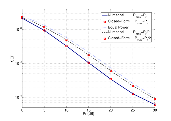
Figure 3: Average SEP obtained based on the proposed exact and approximate power allocation methods and the equal power allocation method with 3 relays.

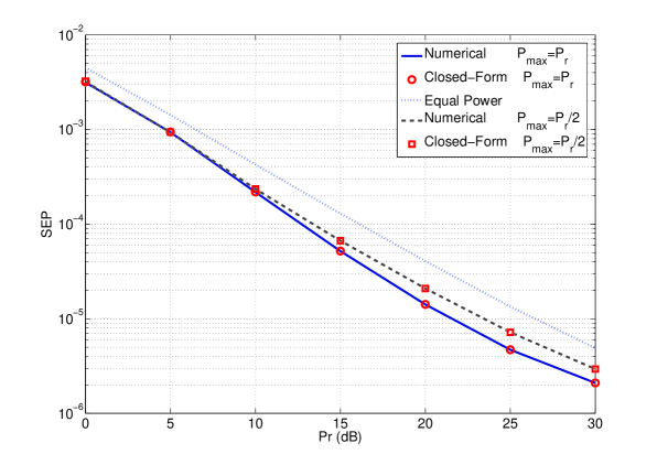
Figure 4: Average SEP obtained based on the proposed exact and approximate power allocation methods and the equal power allocation method with 5 relays.

V-C Performance Improvement Compared to Recent Methods

In our last simulation example, we aim at comparing the performance of our proposed power allocation scheme with another recently proposed power allocation scheme. The other scheme aims at minimizing the power required by all AF relay nodes under the constraint that the average SEP does not exceed a certain desired value and it uses the knowledge of the average channel gains [11]. Thus, as compared to our proposed power allocation scheme, which minimizes the average SEP of a DF cooperative network subject to a fixed total power of the relays nodes, the method of [11] minimizes the total power required by the relay nodes of an AF cooperative network and fix the bound on the average SEP. Both schemes use only the knowledge of the average channel gains.

Compared to the method of [11] according to which all relays always retransmit the source message, our proposed method exploits the additional information about the source message decoding failure/success in each relay node, and thus, not all relays retransmit the message. As a result, it is expected that the proposed method will outperform the one in [11]. In addition, an approximation of SEP, which is accurate only at high SNRs, is used in [11], while the exact SEP expression is derived and used for our power allocation scheme. To ensure a fair comparison between two aforementioned power allocation schemes, we first find optimal power allocation according to the scheme of [11]. Then, we use the total power obtained by the scheme of [11] as a power bound for our proposed power allocation scheme to ensure that the network operates with the same amount of total power in both cases.

Fig. 5 compares the SEP corresponding to the optimal power allocation of the AF cooperative network using [11] and the SEP corresponding to the optimal power allocation obtained based on the proposed method for DF networks for relays $1,3,5$ and all relays $1,2,3,4,5$, respectively, versus different desired SEPs denoted as SEP₀ for the case that there is no restriction on the maximum allowed power for each relay node. Monte-Carlo simulations with $10^{6}$ independent runs are used for obtaining each point in Fig. 5. It can be observed from this figure that, as expected, the proposed power allocation scheme has superior performance over that of the scheme of [11] with the same average transmit power from the relay node. This improvement can be attributed to the fact that in the proposed scheme the relay for which the channel condition between the source and relay is not good enough or, equivalently, the relay that can not decode the source message correctly, does not transmit. This additional information is exploited in the proposed scheme, while it is not used in the scheme of [11]. In addition, the exact average SEP is used for the proposed scheme versus the approximate one in the scheme of [11].

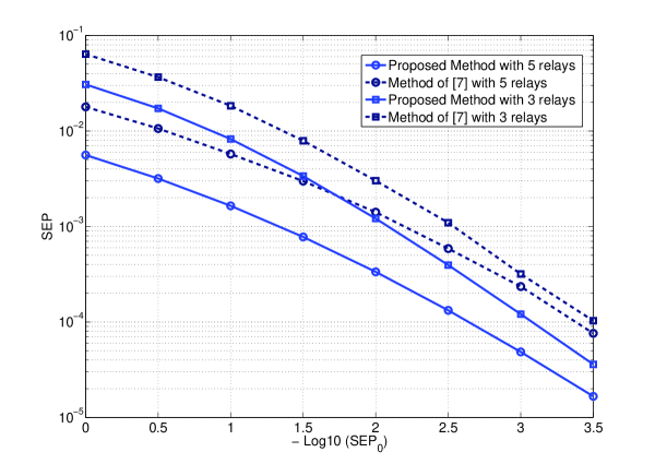
Figure 5: Average SEP obtained based on the proposed approximate power allocation method and the method of [11] using $3$ and $5$ relays.

VI Conclusion

A new simple closed form expression for the average SEP for DF cooperative relay network has been derived. Using this expression, a new power allocation scheme for DF relay networks has been developed by minimizing the average SEP under the constraints on the total power of all relays and the maximum powers of individual relays. The proposed scheme requires only the knowledge of the average of the channel gains from relays to destination and the direct link. The exact and approximate closed form solutions to the corresponding optimization problem have been found and a high accuracy of an approximate solution is demonstrated. According to the proposed approximate solution, the power allocation and relay admission depend on the average probability of correct decoding by relay nodes and also on the corresponding average channel gain-to-noise ratios for admitted relays. The improved performance of the proposed scheme compared to some other schemes is convincingly shown via simulations.

Appendix A

Let us consider the following formula for the average SEP

$$P_{e}\!\!\! = \!\!\!\frac{1}{\pi}\sum_{k=0}^{2^{N}-1}\bigg{(}\prod_{\{i|\boldsymbol{\phi}_{k}(i)=1\}\cup\{i=0\}}\!\beta_{i}\cdot\prod_{\{i|\boldsymbol{\phi}_{k}(i)=0\}}\!(1\!-\!\beta_{i})$$ (51)

$$\times \!\!\!\int_{0}^{\frac{M-1}{M}\pi}\!\prod_{\{i|\boldsymbol{\phi}_{k}(i)=1\}\cup\{i=0\}}\frac{\sin^{2}(\theta)}{\sin^{2}(\theta)\!+\!b_{i}p_{i}}d\theta\bigg{)}.$$

The Hessian of the integral inside (51) with respect to $\mathbf{p}$ can be obtained as

$$\mathbf{H}\!\!\! = \!\!\!\frac{1}{\pi}\int_{0}^{\frac{M-1}{M}\pi}\bigg{(}\mathbf{a}_{\boldsymbol{\phi}(k)}(\theta,\mathbf{p})\mathbf{a}_{\boldsymbol{\phi}(k)}^{H}(\theta,\mathbf{p})$$ (52)

$$+ \!\!\!\mathbf{D}_{\boldsymbol{\phi}(k)}(\theta,\mathbf{p}))g_{\boldsymbol{\phi}(k)}(\theta,\mathbf{p})\bigg{)}\,d\theta$$

where

$$g_{{\boldsymbol{\phi}}_{k}}(\theta,\mathbf{p})=\prod_{\{i|\boldsymbol{\phi}_{k}(i)=1\}\cup\{i=0\}}\frac{\sin^{2}(\theta)}{\sin^{2}(\theta)+b_{i}p_{i}}$$ (53)

$$\mathbf{a}_{\boldsymbol{\phi}_{k}}(\theta,\mathbf{p})\triangleq\left(\frac{b_{1}\boldsymbol{\phi}_{k}(1)}{\sin^{2}(\theta)+b_{1}p_{1}},\cdots,\frac{b_{N}\boldsymbol{\phi}_{k}(N)}{\sin^{2}(\theta)+b_{N}p_{N}}\right)^{T}$$ (54)

$$\!\!\!\mathbf{D}_{\boldsymbol{\phi}(k)}(\theta,\mathbf{p})\!\triangleq$$

$$\!\!\!diag\left(\!\frac{{b_{1}}^{2}\boldsymbol{\phi}_{k}(1)}{(\sin^{2}(\theta)\!\!+\!\!b_{1}p_{1})^{2}},\!\cdots,\!\frac{{b_{N}}^{2}\boldsymbol{\phi}_{k}(N)}{(\sin^{2}(\theta)\!\!+\!\!b_{N}p_{N})^{2}}\!\right)$$ (55)

with $(\cdot)^{H}$ denoting the Hermitian transpose and $diag(\cdot)$ standing for a diagonal matrix.

Since the matrices $\mathbf{a}_{\boldsymbol{\phi}_{k}}(\theta,\mathbf{p})\mathbf{a}_{\boldsymbol{\phi}_{k}}^{H}(\theta,\mathbf{p})$ and $\mathbf{D}_{\boldsymbol{\phi}_{k}}(\theta,\mathbf{p})$ are both positive semi-definite for $\theta\in\left(0,(M-1)\pi/M\right)$ and $p_{i}\geq 0$, $\ i=1,\cdots,N$ and also $g_{\boldsymbol{\phi}_{k}}(\theta,\mathbf{p})\geq 0$, the Hessian matrix is positive semi-definite. The average SEP (51) is a linear combination of integral expressions that are convex, and as a result, it is convex on nonnegative orthant. Moreover, since the constraints of (25)–(27) are linear and form a convex set which is a subset of nonnegative orthant, the problem (25)–(27) overall is convex. $\hfill\square$

Appendix B

The numerical procedure for solving the problem (25)–(27) is based on the interior-point methods. Specifically, the barrier function method, which is one of the widely used interior-point methods, is applied. The barrier function method for solving the problem (25)–(27) can be summarized in terms of the following algorithm.

Given strictly feasible ${\mathbf{p}}=(p_{1},p_{2},...,p_{N})$, $t=t^{(0)}$, $\mu>1$, and $\epsilon>0$, where $t>0$ is the step parameter of the barrier function method, $\mu$ is the step size of the algorithm, and $\epsilon$ is the allowed duality gap (accuracy parameter) (see [18]), do the following.
   1. Compute $\mathbf{p}(t)\!=\!\arg\min\left\{\frac{t}{\pi}\!\int_{0}^{\frac{M-1}{M}\pi}g(\theta,\mathbf{p})\,d\theta\!-\!\sum_{i=1}^{N}{\log{p_{i}}}\right.$ $\left.-\sum_{i=1}^{N}{\log(p_{i}^{max}-p_{i})}\right\}$ subject to $\sum_{i=1}^{N}{\beta_{i}p_{i}}=p_{R}$ starting at current $\mathbf{p}$ using Newton’s method.
   2. Update $\mathbf{p}:=\mathbf{p}(t)$.
   3. Stopping criterion: quit if ${N}/{t}<\epsilon$
   4. Increase $t=\mu t$ and go to step 1.

In this algorithm, $\mathbf{p}(t)$ is called the central point and the first step of the algorithm is called the centering step. Then, at each iteration the central point $\mathbf{p}(t)$ is recomputed using Newton’s method until $N/t<\epsilon$, that guarantees that the solution is found with accuracy $\epsilon$, i.e., $P_{e}(\mathbf{p})-P_{e}(\mathbf{p}_{opt})<\epsilon$.

For solving the optimization problem in the centering step, which is a convex problem with a linear equality constraint, the extended Newton’s method is applied. It can be summarized as follows.

Use $\mathbf{p}$ as an initial point and select error tolerance used in the Newton’s method $\epsilon_{r}$.
   1. Compute the Newton step $\Delta\mathbf{p}$ and decrement $\lambda(\mathbf{p})$.
   2. Stopping criterion: quit if $\lambda(\mathbf{p})^{2}/2<\epsilon_{r}$.
   3. Line Search: Choose step size $s$ by backtracking line search.
   4. Update $\mathbf{p}:=\mathbf{p}+s\Delta p$ and go to step 1.

The Newton’s step $\Delta\mathbf{p}$ and decrement $\lambda(\mathbf{p})$ are obtained from the following equations

$$\begin{pmatrix}\nabla^{2}H(\mathbf{p})&\mathbf{a}\\ \mathbf{a}^{T}&0\end{pmatrix}\begin{pmatrix}\Delta\mathbf{p}\\ w\end{pmatrix}=\begin{pmatrix}-\nabla H(\mathbf{p})\\ 0\end{pmatrix}$$

where

$$h(\mathbf{p})\!\!\! = \!\!\!\frac{t}{\pi}\int_{0}^{\frac{M-1}{M}\pi}g(\theta,\mathbf{p})\,d\theta$$

$$- \!\!\!\sum_{i=1}^{N}{\log{p_{i}}}-\sum_{i=1}^{N}\log(p_{i}^{max}\!-\!p_{i})$$

and $\nabla^{2}H(\mathbf{p})$ and $\nabla H(\mathbf{p})$ are the Hessian and gradient of $H(\mathbf{p})$, respectively. Finally, decrement is defined as

$$\lambda(\mathbf{p})=(\Delta\mathbf{p}^{T}\nabla^{2}H(\mathbf{p})\Delta\mathbf{p})^{1/2}$$

and $\mathbf{a}=(\beta_{1},\ldots,\beta_{N})$.

Appendix C

First, note that the Lagrange multiplier $\nu^{\prime}$ is non-negative, otherwise the equation (IV-A) implies that $\gamma_{i}^{\prime},\ i=1,\cdots,N$ are all positive numbers and, in turn, equation (44) implies that $p_{i}=p_{i}^{max}$, $i=1,\ldots,N$. Since it was assumed that $\sum^{N}_{i=1}\beta_{i}{p_{i}^{max}}>p_{R}$, the condition (48) can not be satisfied for negative $\nu^{\prime}$. As a result, $\nu^{\prime}$ must be non-negative. Depending on whether $b_{i}$ is greater or smaller than ${\nu}^{\prime}$, two cases are possible. If $b_{i}\leq{\nu}^{\prime}$, then the condition (IV-A) holds true only if $p_{i}=0$. Indeed, if $b_{i}\leq{\nu}^{\prime}$, the expression $\beta_{i}{\nu}^{\prime}+{{\gamma}_{i}}^{\prime}-\beta_{i}b_{i}/(\beta_{i}(1+b_{i}p_{i})+(1-\beta_{i})(1+b_{i}p_{i})^{2})$ equals to the non-negative quantity $\beta_{i}{\nu}^{\prime}+{{\gamma}_{i}}^{\prime}-\beta_{i}b_{i}$ when $p_{i}=0$. Furthermore, by considering the fact that the term $\beta_{i}b_{i}/\left(\beta_{i}(1+b_{i}p_{i})+(1-\beta_{i})(1+b_{i}p_{i})^{2}\right)$ is strictly decreasing with respect to $p_{i}$, it is resulted that the expression $\beta_{i}{\nu}^{\prime}+{{\gamma}_{i}}^{\prime}-\beta_{i}b_{i}/(\beta_{i}(1+b_{i}p_{i})+(1-\beta_{i})(1+b_{i}p_{i})^{2})$ is greater than zero if $p_{i}>0$, which means that the condition (IV-A) can not be satisfied if $p_{i}>0$. Thus, $p_{i}$ is zero when ${b}_{i}\leq{\nu}^{\prime}$. Furthermore, if $b_{i}>{\nu}^{\prime}$, then $p_{i}$ can not be equal to 0. It is because if $p_{i}$ equals zero then the condition (44) implies that ${{\gamma}_{i}}^{\prime}=0$. Then, substituting $p_{i}=0$ and ${{\gamma}_{i}}^{\prime}=0$ in the condition (IV-A) yields that $b_{i}\leq{\nu}^{\prime}$, which contradicts the condition ${\ b}_{i}>{\nu}^{\prime}$. Therefore, using the condition (IV-A) and the fact that $p_{i}$ must be positive if ${\ b}_{i}>{\nu}^{\prime}$ we can infer that

$$\beta_{i}{\nu}^{\prime}+{{\gamma}_{i}}^{\prime}-\frac{\beta_{i}b_{i}}{\beta_{i}(1+b_{i}p_{i})+(1-\beta_{i})(1+b_{i}p_{i})^{2}}\ \!=\!0$$ (56)

By solving (56) with respect to $p_{i}$, we can find that

$${\ p}_{i}\!\!\! = \!\!\!\frac{1}{b_{i}}\left(\frac{-\beta_{i}\!+\!\sqrt{\beta_{i}^{2}\!+\!4\beta_{i}(1\!-\!\beta_{i})b_{i}/({\beta_{i}\nu}^{\prime}\!+\!{\gamma}_{i}^{\prime})}}{2(1\!-\!\beta_{i})}\!-\!1\right)$$ (57)

$$\triangleq \!\!\!f_{i}(\nu^{\prime},{\gamma}_{i}^{\prime}).$$

Note that the negative root is not considered because $p_{i}$ must be non-negative. We also defined above the function $f_{i}(\nu^{\prime},{\gamma}_{i}^{\prime})$ for notation simplicity. By substituting the latter expression for ${\ p}_{i}$ into (44) and (47), we obtain

$${{\gamma}_{i}}^{\prime}\left(f_{i}(\nu^{\prime},{\gamma}_{i}^{\prime})-{p_{i}}^{max}\right)=0$$ (58)

$$0\leq f_{i}(\nu^{\prime},{\gamma}_{i}^{\prime})\leq{p_{i}}^{max}.$$ (59)

If $f_{i}(\nu^{\prime},0)>{p_{i}}^{max}$, then the function $f_{i}(\nu^{\prime},{\gamma}_{i}^{\prime})$ is strictly decreasing with respect to ${\gamma}_{i}^{\prime}$ since $\nu^{\prime}$ is non-negative. Thus, the condition (59) holds true only if ${\gamma}_{i}^{\prime}>0$. In addition, the condition (58) implies that $p_{i}={p_{i}}^{max}$. Then the only remaining case is when $0\leq f_{i}(\nu^{\prime},0)\leq{p_{i}}^{max}$. In this case, the conditions (58) and (59) hold true only if ${{\gamma}_{i}}^{\prime}=0$. Considering the fact that the case of ${b}_{i}\leq{\nu}^{\prime}$ is equivalent to the case when $f_{i}(\nu^{\prime},0)\leq 0$, we can conclude that all possible cases are analyzed and they then can be summarized as (49). $\square$

References

• [1] Y. W. Hong, W. J. Huang, F. H. Chiu, and C. C. J. Kuo, “Cooperative communications in resource-constrained wireless networks,” IEEE Signal Porcessing Mag., vol. 24, no. 3, pp. 47 -57, May 2007.
• [2] J. N. Laneman, D. N. C. Tse, and G. W. Wornell, “Cooperative diversity in wireless networks: Efficient protocols and outage behavior,” IEEE Trans. Inf. Theory, vol. 50, no. 12, pp. 3062 -3080, Dec. 2004.
• [3] K. T. Phan, T. Le-Ngoc, S. A. Vorobyov, and C. Tellambura, “Power allocation in wireless multi-user relay networks,” IEEE Trans. Wireless Commun., vol. 8, no. 5, pp. 2535–2545, May 2009.
• [4] A. Goldsmith, Wireless Communications. Cambridge University Press: Cambridge, 2005.
• [5] K. T. Phan, S. A. Vorobyov, and C. Tellambura, “Precoder design for space-time coded MIMO systems with correlated Rayleigh fading channels using convex optimization,” IEEE Trans. Signal Processing, vol. 57, no. 2, pp. 814–819, Feb. 2009.
• [6] M. Chen, S. Serbetli, and A. Yener, “Distributed power allocation strategies for parallel relay networks,” IEEE Trans. Wireless Commun., vol. 7, no. 2, pp. 552- 561, Feb. 2008.
• [7] Y. Zhao, R. Adve, and T. J. Lim, “Improving amplify-and-forward relay networks: Optimal power allocation versus selection,” IEEE Trans. Wireless Commun., vol. 6, no. 8, pp. 3114 -3123, Aug. 2007.
• [8] A. Bletsas, A. Khisti, D. P. Reed, and A. Lippman, “A simple cooperative method based on network path selection,”IEEE Journal on Selected Areas in Communications, vol. 24, no. 3,pp. 659- 672, Mar. 2006.
• [9] A. Host-Madsen and J. Zhang, “Capacity bounds and power allocation for wireless relay channels,”IEEE Trans. Inform. Theory, vol. 51, no. 6, pp. 2020 -2040, Jun. 2005.
• [10] J. Luo, R. S. Blum, L. Cimini, L. Greenstein, and A. Haimovich, “Power allocation in a transmit diversity system with mean channel gain information,” IEEE Commun. Lett., vol. 9, pp. 616–618, Jul. 2005.
• [11] B. Maham, A. Hjorungnes, and M. Debbah, “Power allocations in minimum-energy SER constrained cooperative networks,” special issue on cognitive radio, Annals of telecommunications - Annales des t l communications, vol. 64, no. 7, pp. 545–555, Aug. 2009.
• [12] W.  Su, A. K. Sadek, K. J. R. Liu, “SER performance analysis and optimum power allocation for decode-and-forward cooperation protocol in wireless networks,” in Proc. IEEE Wireless Communications and Networking Conf., New Orleans, LA, USA, Mar. 2005, pp. 984–989.
• [13] A. K. Sadek, W. Su, K. J. R. Liu, “Multinode cooperative communications in wireless networks,” IEEE Trans. on Signal Processing, vol. 55, no. 1, pp. 341–355, Jan. 2007.
• [14] Y.  Lee, M. H. Tsai, S. L.  Sou, “Performance of decode-and-forward cooperative communications with multiple dual-hop relays over nakagami-m fading channels,” IEEE Trans. on Wireless Commun., vol. 8, no. 6, pp. 2853–2859, June 2009.
• [15] A. Khabbazibasmenj and S. A. Vorobyov, “Power allocation in decode-and-forward cooperative networks via SEP minimization,” in Proc. 3rd IEEE CAMSAP, Aruba, Dutch Antilles, Dec. 2009, pp. 328–331.
• [16] P. Vandewalle, J. Kovacevic, and M. Vetterli, “Reproducible research in signal processing,” IEEE Signal Process. Mag., vol. 26, no. 3, pp. 37 47, May 2009.
• [17] M. K. Simon and M.-S. Alouini, “A unified approach to the performance analysis of digital communication over generalized fading channels,” Proc. IEEE, vol. 86, pp. 1860 -1877, Sept. 1998.
• [18] S. Boyd and L. Vandenberghe, Convex Optimization. Cambridge University Press: Cambridge, 2004.