$\mathcal{P}\mathcal{T}$-Symmetric Representations of Fermionic Algebras

Abstract

A recent paper by Jones-Smith and Mathur extends $\mathcal{P}\mathcal{T}$-symmetric quantum mechanics from bosonic systems (systems for which $\mathcal{T}^{2}={\bf 1}$) to fermionic systems (systems for which $\mathcal{T}^{2}=-{\bf 1}$). The current paper shows how the formalism developed by Jones-Smith and Mathur can be used to construct $\mathcal{P}\mathcal{T}$-symmetric matrix representations for operator algebras of the form $\eta^{2}=0$, $\bar{\eta}^{2}=0$, $\eta\bar{\eta}+\bar{\eta}\eta=\alpha{\bf 1}$, where $\bar{\eta}=\eta^{\mathcal{P}\mathcal{T}}=\mathcal{P}\mathcal{T}\eta\mathcal{T}^{-1}\mathcal{P}^{-1}$. It is easy to construct matrix representations for the Grassmann algebra ($\alpha=0$). However, one can only construct matrix representations for the fermionic operator algebra ($\alpha\neq 0$) if $\alpha=-1$; a matrix representation does not exist for the conventional value $\alpha=1$.

I Introduction

A recent paper X1 shows how to generalize $\mathcal{P}\mathcal{T}$ quantum mechanics from the Heisenberg algebra $[q,p]=i$ to other kinds of algebras, such as E2. (The E2 algebra is characterized by a set of three commutation relations: $[u,J]=iv$, $[v,J]=-iu$, $[u,v]=0$.) The algebras considered in Ref. X1 are bosonic in character because they are expressed in terms of commutation relations. However, Jones-Smith and Mathur have shown how to describe $\mathcal{P}\mathcal{T}$-symmetric quantum theories in a fermionic setting X2 . Thus, in the current paper we apply the formalism developed in Ref. X2 to examine the representations of algebras expressed in terms of anticommutation relations.

We consider here two standard algebras: the operator algebra of fermions, which consists of two nilpotent elements, $\eta$ and $\bar{\eta}$, whose anticommutator is unity,

$$\eta^{2}=0,\quad\bar{\eta}^{2}=0,\quad\eta\bar{\eta}+\bar{\eta}\eta={\bf 1},$$ (1)

and the Grassmann algebra, which again consists of two nilpotent elements, $\eta$ and $\bar{\eta}$, whose anticommutator vanishes,

$$\eta^{2}=0,\quad\bar{\eta}^{2}=0,\quad\eta\bar{\eta}+\bar{\eta}\eta=0.$$ (2)

The requirement that $\eta$ and $\bar{\eta}$ be nilpotent is imposed to incorporate fermionic statistics. Our objective is to find matrix representations of (1) and (2) in the context of fermionic $\mathcal{P}\mathcal{T}$-symmetric quantum mechanics; that is, under the assumption that $\bar{\eta}$ is the $\mathcal{P}\mathcal{T}$ reflection of $\eta$:

$$\bar{\eta}=\mathcal{P}\mathcal{T}\eta\mathcal{T}^{-1}\mathcal{P}^{-1}.$$ (3)

In Sec. II we investigate the two-dimensional matrix representations of (1) and (2) using nothing more than the representation of $\mathcal{P}$ and $\mathcal{T}$ introduced in Ref. X3 in which the square of the $\mathcal{T}$ operator is unity: $\mathcal{T}^{2}={\bf 1}$. Then in Sec. III, we apply the more elaborate formalism introduced recently in Ref. X2 in which is it argued that $\mathcal{T}^{2}=-{\bf 1}$ (and not ${\bf 1}$) for fermions. We show that if we replace the condition $\mathcal{T}^{2}={\bf 1}$ by $\mathcal{T}^{2}=-{\bf 1}$, it is still possible to find matrix representations of the Grassmann algebra (2). However, the surprise is that it is not possible to find matrix representations of the fermion operator algebra in (1); one can only find matrix representations of the $\mathcal{P}\mathcal{T}$ version of the fermionic operator algebra

$$\eta^{2}=0,\quad\bar{\eta}^{2}=0,\quad\eta\bar{\eta}+\bar{\eta}\eta=-{\bf 1}.$$ (4)

II Two-dimensional representations of $\eta$ and $\bar{\eta}$

For purposes of comparison, we begin by considering a two-dimensional matrix representation in which we assume that $\bar{\eta}$ is given by the conventional Hermitian adjoint $\bar{\eta}=\eta^{\dagger}$. The most general complex matrix $\eta$ whose square vanishes has vanishing trace and determinant,

$$\eta=\left(\begin{array}[]{cc}a&b\cr c&-a\cr\end{array}\right),$$ (5)

where $b$ and $c$ are arbitrary complex numbers and $a$ is fixed by the determinant condition $a^{2}+bc=0$. Then, $\bar{\eta}$ is given by

$$\bar{\eta}=\left(\begin{array}[]{cc}a^{*}&c^{*}\cr b^{*}&-a^{*}\cr\end{array}\right)$$ (6)

and the nilpotency condition $\bar{\eta}^{2}=0$ is automatically satisfied. The fermionic algebra condition $\eta\bar{\eta}+\bar{\eta}\eta={\bf 1}$ now reduces to

$$|b|+|c|=1.$$ (7)

Thus, if $b$ and $c$ are real, they are constrained to a unit diamond, as shown in Fig. 1. More generally, if $b=ue^{i\alpha}$ and $c=ve^{i\beta}$ are complex, then $\alpha$ and $\beta$ are arbitrary and $u\geq 0$ and $v\geq 0$ lie on the line segment $u+v=1$ in the positive quadrant of the $(u,v)$ plane.

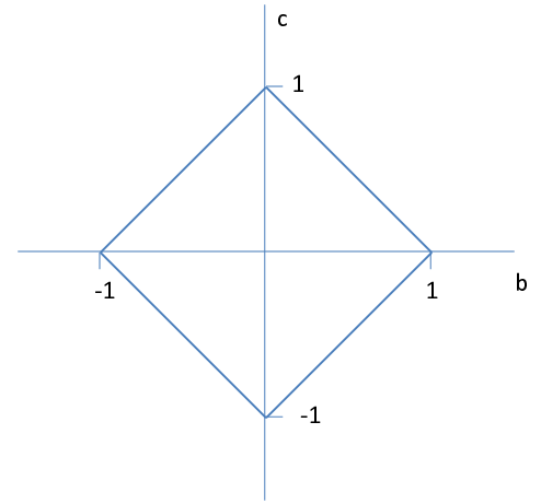
Figure 1: Plot of the real parameters $b$ and $c$ for the representation of $\eta$ in (5) for the case in which $\bar{\eta}$ is the conventional Hermitian conjugate of $\eta$; $\eta$ and $\bar{\eta}$ satisfy the fermionic algebra $\eta\bar{\eta}+\bar{\eta}\eta={\bf 1}$. The diamond-shaped locus of points is described by the equation $|b|+|c|=1$.

For the case of the Grassmann algebra, $b$ and $c$ satisfy the constraint

$$|b|+|c|=0$$ (8)

instead of (7). The unique solution to (8) is $b=c=0$. Thus, in this case there is no nontrivial Grassmann representation for $\eta$ and $\bar{\eta}$.

Now let us turn to the case of a $\mathcal{P}\mathcal{T}$-symmetric fermionic algebra. What happens if we apply to fermions the naive representations of parity reflection $\mathcal{P}$ and time reversal $\mathcal{T}$ that were used earlier in Ref. X3 ? We represent a parity reflection as a real symmetric matrix whose square is unity, which for two-dimensional matrices is

$$\mathcal{P}=\left(\begin{array}[]{cc}0&1\cr 1&0\cr\end{array}\right)$$ (9)

and we represent $\mathcal{T}$ as complex conjugation. With these choices, $\mathcal{P}^{2}=1$, $\mathcal{T}^{2}=1$, and $[\mathcal{P},\mathcal{T}]=0$.

Here, if $\eta$ is as given in (5), then from (3) $\bar{\eta}$ is given by

$$\bar{\eta}=\mathcal{P}\mathcal{T}\eta\mathcal{P}\mathcal{T}=\left(\begin{array}[]{cc}-a^{*}&c^{*}\cr b^{*}&a^{*}\cr\end{array}\right).$$ (10)

Once again, the condition $\bar{\eta}^{2}=0$ is automatically satisfied. Now, requiring that $\eta$ and $\bar{\eta}$ obey the fermionic algebra $\eta\bar{\eta}+\bar{\eta}\eta=1$ leads to the condition

$$(|b|-|c|)^{2}=1.$$ (11)

Thus, if $b$ and $c$ are real, they lie on the lines shown in Fig. 2, which is the unbounded extended complement of the diamond shown in Fig. 2. More generally, if $b=ue^{i\alpha}$ and $c=ve^{i\beta}$ are complex, then $\alpha$ and $\beta$ are arbitrary, and $u\geq 0$ and $v\geq 0$ lie on two infinite lines $u-v=\pm 1$ in the positive quadrant of the $(u,v)$ plane.

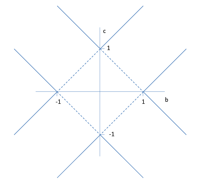
Figure 2: Plot of the real parameters $b$ and $c$ for the representation of $\eta$ in (5) for the case in which $\bar{\eta}$ is the $\mathcal{P}\mathcal{T}$ conjugate of $\eta$, where $\mathcal{P}$ is given in (9) and $\mathcal{T}$ is complex conjugation, $\eta$ and $\bar{\eta}$ satisfy a fermionic algebra. The locus of points is described by the equation $(|b|-|c|)^{2}=1$ and is thus an unbounded region, in contrast with the bounded region shown in Fig. 1.

If $\eta$ and $\bar{\eta}$ are required to satisfy a Grassmann algebra, then if $b$ and $c$ are real, they must satisfy the equation

$$|b|-|c|=0.$$ (12)

Thus, unlike the Hermitian case, there is a nontrivial set of solutions.

It is interesting that when $\bar{\eta}$ is the $\mathcal{P}\mathcal{T}$ conjugate of $\eta$, there is an unbounded range of parameters and that when $\bar{\eta}$ is the Hermitian conjugate of $\eta$, the range of parameters is bounded. This result is strongly analogous to what was found in the study of the $\mathcal{P}\mathcal{T}$-symmetric quantum brachistochrone compared with the conventional Hermitian quantum brachistochrone X4 . The matrix elements of the Hamiltonian that describes the $\mathcal{P}\mathcal{T}$ brachistochrone are unbounded (even though the eigenvalues are fixed), while the matrix elements of the Hamiltonian for the Hermitian quantum brachistochrone are bounded. Thus, $\mathcal{P}\mathcal{T}$-symmetric quantum mechanics is hyperbolic (unbounded) in character, while conventional Hermitian quantum mechanics is elliptic (bounded) in character.

III Application of the Formalism of Jones-Smith and Mathur

For a correct quantum-mechanical description of fermions, the time-reflection operator $\mathcal{T}$ must be chosen such that its square is $-{\bf 1}$ instead of ${\bf 1}$ X5 . In a recent paper by Jones-Smith and Mathur, this fact is used to construct suitable matrix representations of the $\mathcal{T}$ and $\mathcal{P}$ operators X2 . In the following subsection we briefly recapitulate their results.

III.1 Brief summary of the essential results of Jones-Smith and Mathur

In Ref. X2 it is shown how to construct matrix representations of dimension $4n$ $(n=1,\,2,\,3,\,\ldots)$ of the $\mathcal{T}$ and $\mathcal{P}$ operators. The effect of a time operator acting on a state $\psi$, which is a $4m$-dimensional vector, is to take the complex conjugate of $\psi$ and to multiply the result by a real matrix $t$:

$$\mathcal{T}\psi=t\psi^{*}.$$ (13)

The general form for the $t$ matrix consists of $2n$ copies of the $2\times 2$ matrix

$$\left(\begin{array}[]{cc}0&1\cr-1&0\cr\end{array}\right)$$

on the main diagonal and zero entries elsewhere. For the simplest ($n=1$) case $t$ is the $4\times 4$ matrix

$$t=\left(\begin{array}[]{cccc}0&1&0&0\cr-1&0&0&0\cr 0&0&0&1\cr 0&0&-1&0\cr\end{array}\right).$$ (14)

The effect of a parity operator acting on a state $\psi$ is to multiply $\psi$ by a real matrix $p$:

$$\mathcal{P}\psi=p\psi.$$ (15)

The general form for the $p$ matrix is the diagonal matrix whose first $2n$ diagonal elements are $1$ and whose next $2n$ diagonal elements are $-1$. For the simplest ($n=1$) case $p$ is the $4\times 4$ matrix

$$p=\left(\begin{array}[]{cccc}1&0&0&0\cr 0&1&0&0\cr 0&0&-1&0\cr 0&0&0&-1\cr\end{array}\right).$$ (16)

Note that with these choices the operators $\mathcal{P}$ and $\mathcal{T}$ commute, $\mathcal{P}^{2}={\bf 1}$, and $\mathcal{T}^{2}=-{\bf 1}$. Also, the matrices $p$ and $t$ satisfy $[p,t]=0$, $p^{2}={\bf 1}$, and $t^{2}=-{\bf 1}$.

These results are nearly identical with those of Bjorken and Drell X6 in their discussion of the operators $\mathcal{P}$ and $\mathcal{T}$ for the Dirac equation. In this text it is shown that when the parity-reflection operator $\mathcal{P}$ acts on a four-component spinor, it has the effect of multiplying the spinor by the matrix $\gamma^{0}$, which is precisely the matrix $p$ given in (16). Furthermore, when the time-reversal operator $\mathcal{T}$ acts on a four-component spinor, it has the effect of multiplying the spinor by the matrix $i\gamma^{1}\gamma^{3}$, which is the matrix $\tau=it$, with $t$ given in (14). Thus, $\tau^{2}={\bf 1}$. It still follows that $\mathcal{T}^{2}=-{\bf 1}$ because $\tau$ is imaginary and thus it changes sign under complex conjugation.

III.2 Construction of quadratically nilpotent matrices

Our next task is to construct general classes of quadratically nilpotent matrices. We know that an $n$-dimensional matrix whose square vanishes must have a vanishing trace and determinant. Of course, if $n>2$, not all traceless $n$-dimensional matrices having a vanishing determinant are quadratically nilpotent. Thus, we propose the following very simple general set of such matrices: Let the elements in the top row of the matrix be arbitrarily chosen complex numbers: $a_{1},\,a_{2},\,a_{3},\ldots,a_{n}$. Next, let the $k$th row ($k>1$) be an arbitrary multiple $b_{k}$ of the elements in the first row. This matrix contains $2n-1$ arbitrary complex parameters and by construction its determinant vanishes.

We then impose the condition that the matrix be traceless:

$$a_{1}+a_{2}b_{2}+a_{3}b_{3}+\ldots+a_{n}b_{n}=0.$$ (17)

The resulting matrix contains $2n-2$ complex parameters and is quadratically nilpotent. In four dimensions this construction gives the following general 12-parameter complex matrix representation for $\eta$:

$$\eta=\left(\begin{array}[]{cccc}-ch-bg-af&f&g&h\cr-a(ch+bg+af)&af&ag&ah\cr-b(ch+bg+af)&bf&bg&bh\cr-c(ch+bg+af)&cf&cg&ch\cr\end{array}\right).$$ (18)

Using the matrix representation in (14) for the time-reversal operator and the matrix representation $p$ in (16) for the parity-reflection operator, we obtain from (3) the $\mathcal{P}\mathcal{T}$ reflection of $\eta$ from the formula $\bar{\eta}=-p\,t\,\eta^{*}\,t\,p$ X7 :

$$\bar{\eta}=\left(\begin{array}[]{cccc}af&a(ch+bg+af)&-ah&ag\cr-f&-ch-bg-af&h&-g\cr-cf&-c(ch+bg+af)&ch&-cg\cr bf&b(ch+bg+af)&-bh&bg\cr\end{array}\right)^{*}.$$ (19)

One can verify that $\bar{\eta}^{2}=0$.

III.3 Grassmann algebra

Using the $4\times 4$ matrix representations for $\eta$ in (18) and $\bar{\eta}$ in (19), we can now construct the anticommutator $y=\eta\bar{\eta}+\bar{\eta}\eta$. For the special case in which the parameters $a$, $b$, $c$, $f$, $g$, $h$ are real, the matrix $y$ has a particularly simple form because the expression $ach-bh+cg+abg+a^{2}f+f$ factors out of all 16 matrix elements:

$$y=(ach-bh+cg+abg+a^{2}f+f)\left(\begin{array}[]{cccc}-ach-abg-a^{2}f-f&-ch-bg&h+ag&ah-g\cr ch+bg&-ach-abg-a^{2}f-f&ah-g&-h-ag\cr c^{2}h+bcg+acf-bf&-bch-b^{2}g-cf-abf&bh-cg&-ch-bg\cr-bch-b^{2}g-cf-abf&-c^{2}h-bcg-acf+bf&ch+bg&bh-cg\cr\end{array}\right).$$ (20)

Thus, if we choose

$$f=(bh-ach-cg-abg)/(a^{2}+1),$$ (21)

then all 16 matrix elements of $y$ vanish, and we have found a five-parameter four-dimensional real matrix representation of $\eta$ and $\bar{\eta}$ for the Grassmann algebra (2).

There is no choice of parameters for which $y={\bf 1}$. To show that this is true, we see from (20) that $y_{2,3}=0$ requires that $g=ah$ and that $y_{2,4}=0$ requires that $h=-ag$. Combining these two equations gives $g(a^{2}+1)=0$. Thus, $g=0$ and also $h=0$. It follows that $y_{4,4}=0$ and we conclude that it is impossible to construct a real matrix representation of $\eta$ that obeys the $\mathcal{P}\mathcal{T}$-symmetric fermionic operator algebra (1).

In general, the parameters in (18) and (19) are complex numbers: $a=a_{1}+a_{2}i$, $b=b_{1}+b_{2}i$, $c=c_{1}+c_{2}i$, $f=f_{1}+f_{2}i$, $g=g_{1}+g_{2}i$, $h=h_{1}+h_{2}i$. If we set the $(1,2)$ matrix element of the anticommutator matrix $y$ to $0$, we obtain two equations for the vanishing of the real and imaginary part. These equations are long and complicated and they are quadratic in all of the parameters $a_{1}$, $a_{2}$, $b_{1}$, $b_{2}$, $\ldots$, except for two; surprisingly, they are linear in $f_{1}$ and $f_{2}$. If we solve this pair of equations simultaneously, we obtain startlingly simple results for the real and imaginary parts of $f$:

$$f_{1} = [(a_{1}c_{2}-a_{2}c_{1}+b_{2})h_{2}+(-a_{2}c_{2}-a_{1}c_{1}+b_{1})h_{1}$$

$$+(-c_{2}+a_{1}b_{2}-a_{2}b_{1})g_{2}+(-c_{1}-a_{2}b_{2}-a_{1}b_{1})g_{1}]$$

$$/(a_{2}^{2}+a_{1}^{2}+1),$$

$$f_{2} = -[(a_{2}c_{2}+a_{1}c_{1}-b_{1})h_{2}+(a_{1}c_{2}-a_{2}c_{1}+b_{2})h_{1}$$ (22)

$$+(c_{1}+a_{2}b_{2}+a_{1}b_{1})g_{2}+(-c_{2}+a_{1}b_{2}-a_{2}b_{1})g_{1}]$$

$$/(a_{2}^{2}+a_{1}^{2}+1).$$

This is the complex generalization of (21).

Substituting $f_{1}$ and $f_{2}$ into $y$, we find that all 16 matrix elements of $y$ vanish. Thus, we have found a 10-parameter complex Grassmann representation. An interesting special case is the complex symmetric representation (there is no real symmetric representation):

$$\eta=\left(\begin{array}[]{cccc}-i&-i\alpha&1&\alpha\cr-i\alpha&-i\alpha^{2}&\alpha&\alpha^{2}\cr 1&\alpha&i&i\alpha\cr\alpha&\alpha^{2}&i\alpha&i\alpha^{2}\cr\end{array}\right),$$ (23)

for which $\alpha$ is real. This representation has an obvious quaternionic structure.

III.4 The Peculiar $\mathcal{P}\mathcal{T}$-Symmetric Fermionic case

To construct a fermionic algebra (for which the matrix $y$ is nonvanishing), we must not allow $f_{1}$ and $f_{2}$ to take the values in (22). The expressions for the matrix elements of $y$ are extremely complicated, but (22) indicates a way to proceed. Note that the denominator of (22) is quadratic in $a_{1}$ and $a_{2}$. This suggests that we should choose $f_{1}=0$ and $f_{2}=0$ so that we can obtain linear equations to solve for $a_{1}$ and $a_{2}$. We find that it is simplest to solve simultaneously the real and imaginary parts of $y_{3,4}=0$ for $a_{1}$ and $a_{2}$ and we obtain

$$a_{1}=N_{1}/D,\qquad a_{2}=N_{2}/D,$$ (24)

where

$$N_{1}=(b_{1}g_{1}-b_{2}g_{2}+c_{1}h_{1}-c_{2}h_{2})(b_{1}h_{1}+b_{2}h_{2}-c_{1}g_{1}-c_{2}g_{2})+(b_{1}g_{2}+b_{2}g_{1}+c_{1}h_{2}+c_{2}h_{1})(b_{1}h_{2}-b_{2}h_{1}-c_{1}g_{2}+c_{2}g_{1}),$$

$$N_{2}=(b_{1}h_{2}-b_{2}h_{1}-c_{1}g_{2}+c_{2}g_{1})(b_{2}g_{2}-b_{1}g_{1}-c_{1}h_{1}+c_{2}h_{2})+(b_{1}h_{1}+b_{2}h_{2}-c_{1}g_{1}-c_{2}g_{2})(b_{1}g_{2}+b_{2}g_{1}+c_{1}h_{2}+c_{2}h_{1}),$$

$$D=(c_{2}h_{2}+b_{2}g_{2}-c_{1}h_{1}-b_{1}g_{1})^{2}+(c_{2}h_{1}+b_{1}g_{2}+c_{1}h_{2}+b_{2}g_{1})^{2}.$$

Amazingly, it is not necessary to solve for any other parameters; we find that when we substitute the values of $a_{1}$ and $a_{2}$ in (24) into the matrix $y$ we obtain after massive simplification a stunningly simple expression for $y$:

$$y=\eta\bar{\eta}+\bar{\eta}\eta=\left(\begin{array}[]{cccc}-1&0&0&0\cr 0&-1&0&0\cr 0&0&-1&0\cr 0&0&0&-1\cr\end{array}\right).$$ (25)

This result is a surprise because $y=-{\bf 1}$ rather than the expected matrix $\bf 1$. Evidently, it is not possible to achieve the conventional fermionic algebra in (1) but rather we get the $\mathcal{P}\mathcal{T}$-symmetric variant of this algebra in (4). Indeed, we have found an eight-parameter representation of this algebra in which the real and imaginary parts of $b$, $c$, $g$, and $h$ are arbitrary. Note that we cannot change the sign in this algebra from $-1$ back to $+1$ by multiplying $\eta$ by a complex phase because the time-reversal operator $\mathcal{T}$ performs complex conjugation.

We conclude that because the time operator for fermions obeys the equation $\mathcal{T}^{2}=-{\bf 1}$, the fermionic operator algebra for a $\mathcal{P}\mathcal{T}$-symmetric system necessarily picks up an extra minus sign; we must replace the algebra in (1) by its $\mathcal{P}\mathcal{T}$ variant in (4). We interpret the negative sign in the fermionic algebra (4) as indicating a fundamental change in character from elliptic to hyperbolic. This is the same interpretation that we presented at the end of Sec. II for the case of a $2\times 2$ $\mathcal{P}\mathcal{T}$-symmetric matrix representation for $\eta$.

CMB is grateful to the Graduate School at the University of Heidelberg for its hospitality. CMB thanks the U.S. Department of Energy for financial support.

References

- (1) C. M. Bender and R. J. Kalveks, Int. J. Theor. Phys. 50, 955 (2011). For the case of the E2 algebra a Hamiltonian of the form was studied. It was found that there is a region of unbroken symmetry () in which all of the eigenvalues are real and regions of broken symmetry () in which some of the eigenvalues are complex. The work on the E2 algebra has been extended to the E3 algebra by R. J. Kalveks and independently by K. Jones-Smith (private communications) and it was found that there are no qualitative differences between E2 and E3; there are still regions of unbroken and broken symmetry.
- (2) K. Jones-Smith and H. Mathur, Phys. Rev. A 82, 042101 (2010).
- (3) C. M. Bender, D. C. Brody, and H. F. Jones, Am. J. Phys. 71, 1095 (2003).
- (4) C. M. Bender, D. C. Brody, H. F. Jones, and B. K. Meister, Phys. Rev. Lett. 98, 040403 (2007).
- (5) A. Messiah, Quantum Mechanics (John Wiley & Sons, New York, 1962), Vol. II, Chap xv.
- (6) J. D. Bjorken and S. D. Drell, Relativistic Quantum Fields (McGraw-Hill, New York, 1964).
- (7) The minus sign in this formula is crucial. It arises because of the following argument: Let be a four-dimensional matrix operator and let be an arbitrary four-component vector. Then, if we apply to , we obtain . Since is arbitrary, we conclude that .