Soft Wall Model in the Hadronic Medium

We study the holographic QCD in the hadronic medium by using the soft wall model. We discuss the Hawking-Page transition between Reissner-Nordström AdS black hole and thermal charged AdS of which the geometries correspond to deconfinement and confinement phases respectively. We also present the numerical result of the vector and axial vector meson spectra depending on the quark density.

1 Introduction

Holographic QCD offers new approaches to understand the strongly interacting regime of gauge theories based on AdS/CFT duality [1]. The properties of QCD including confinement and chiral symmetry breaking have been discussed in asymptotically AdS geometries [2, 3, 4, 5, 6, 7, 8].

The QCD-like models can be derived in both top-down and bottom-up approaches. There are two methods to construct AdS/QCD background in the bottom-up approach. One is introducing an infrared (IR) cutoff [6, 9, 10, 11, 12, 13, 14], and the other is scaling the action or modifying the background metric by introducing a scalar field or a warp factor so that a smooth IR truncation is induced [15, 16, 17]. The light-front holography [18] is constructed by using the both methods.

The phase transition between the confining and deconfining phases corresponds to the Hawking-Page transition [19] of gravity between thermal AdS (tAdS) at low temperature and the Schwarzschild AdS black hole at high temperature in pure gauge theory [2]. The phase transition of holographic QCD in the hard wall [11] and soft wall model [15] was discussed in [20].

The holographic QCD can be improved by including the chemical potential [21, 22, 23, 24, 25, 26, 27, 28, 29, 30, 31, 32, 33].

The charge of Reissner-Nordström AdS black hole (RNAdS BH) can be interpreted as quark charge when branes fill the bulk [27]. The boundary value of the time-component gauge field is the chemical potential whose dual operator is the quark number density. The gravity dual to deconfining phase of QCD is the RNAdS BH. The thermal charged AdS (tcAdS) space, which is the zero mass limit of the RNAdS BH, was proposed as the dual geometry corresponding to the confining phase of QCD [28]. The Hawking-Page transition between confinement and deconfinement phases was studied in the presence of the chemical potential or the quark density in the hard wall model [28, 29]. It has been also observed that meson mass increases as the quark density increases in the hard wall model [30].

In this report, we first discuss the holographic QCD in the hadronic (or quark) medium by using the soft wall model [15] where a non-dynamical scalar field is introduced to give a smooth IR truncation. The scalar field does not affect the dynamics of the gravity as it scales the full action. We next investigate numerically the spectra of the vector and axial-vector mesons depending on the quark density, where the correct boundary conditions consistent with the analytic result of the vector meson are used.

The rest of this paper is organized as follows. In section 2, we investigate the Hawking-Page transition between RNAdS BH and tcAdS. In section 3, we study the vector and axial vector meson spectra depending on the quark density. In section 4, we summarize our results and discuss issues for future work.

2 Hawking-Page transition in the soft wall model

We consider the holographic QCD in the hadronic (or quark) medium using the soft wall model. According to the AdS/CFT correspondence, the quark number operator in the gauge theory side corresponds to the time-component of the bulk gauge field. So the dual geometry of the hadronic medium should be a five-dimensional spacetime containing some electric charges. There are well-known examples describing the asymptotic AdS space containing the electric charges. One is the Reissner-Nordström AdS black hole (RNAdS BH) corresponding to the deconfining phase described by quarks and gluons in the gauge theory side. The RNAdS BH in Euclidean spacetime signature is

$$ds^{2}=\frac{R^{2}}{z^{2}}\left(f_{RN}(z)dt_{\scriptscriptstyle{E}}^{2}+\frac{1}{f_{RN}(z)}dz^{2}+\delta_{ij}dx^{i}dx^{j}\right),$$ (2.1)

with

$$f_{RN}(z)=1-mz^{4}+q^{2}z^{6},$$ (2.2)

where $i,j$ imply the three-dimensional spatial indices. The parameters $R$, $m$ and $q$ are the AdS radius, the black hole mass and charge, respectively. We follow the convention of [29]. The time-component of the corresponding bulk gauge field is

$$A_{0}=i\left(2\pi^{2}\mu-Qz^{2}\right),$$ (2.3)

where $\mu$ and $Q$ are related to the chemical potential and quark number density in the dual gauge theory. To satisfy the Einstein and Maxwell equations the quark number density $Q$ should be related to the black hole charge $q$

$$Q=\sqrt{\frac{3g^{2}R^{2}}{2\kappa^{2}}}q.$$ (2.4)

In the confining phase the vacuum of the dual gauge theory is filled up with hadronic matter as quarks can not exist alone due to the confinement. The dual geometry of it was found in [28], which is another solution satisfying Einstein and Maxwell equations. It is called a thermal charged AdS (tcAdS) space [28], whose metric in Euclidean signature is

$$ds^{2}=\frac{R^{2}}{z^{2}}\left(f_{tc}(z)dt_{\scriptscriptstyle{E}}^{2}+\frac{1}{f_{tc}(z)}dz^{2}+\delta_{ij}dx^{i}dx^{j}\right),$$ (2.5)

with

$$f_{tc}(z)=1+q^{\prime 2}z^{6}.$$ (2.6)

The time-component of the bulk gauge field is also in the form of (2.3). As will be shown, although this tcAdS solution is singular at $z=\infty$ it does not give any problem to calculate the physical quantities due to the potential barrier caused by the non-dynamical scalar field in the soft wall model.

The Hawking-Page transition in the hadronic medium by using the hard wall model has been investigated [28, 29]. The Hawking-Page transition in the soft wall model is also studied for the case of $q=0$ [15, 20]. We investigate the Hawking-Page transition between the RNAdS BH and tcAdS backgrounds in the soft wall model, which describes the deconfinement phase transition of QCD in the hadronic medium. On these backgrounds, the Euclidean gravity action of the soft wall model is given by

$$S=\int d^{5}x\sqrt{G}e^{-\Phi}\mathrm{Tr}\left[\,\frac{1}{2\kappa^{2}}\,(\,-{\cal{R}}+2\Lambda\,)+\frac{1}{4g^{2}}F_{MN}F^{MN}\,\right],$$ (2.7)

where the non-dynamical scalar field is $\Phi=cz^{2}$. According to the AdS/CFT correspondence, the on-shell gravity action corresponds to the thermodynamic energy of the dual gauge theory, so we evaluate the on-shell gravity action on (2.1) and (2.5) with the gauge field (2.3).

For the deconfining phase, which is dual to the RNAdS BH, we impose the Dirichlet boundary condition $A_{0}=i2\pi^{2}\mu$ at the boundary $z=0$ to get the corresponding on-shell gravity action

$$S_{RN}=\frac{R^{3}V_{3}}{\kappa^{2}}\int_{0}^{\beta_{RN}}dt_{\scriptscriptstyle{E}}\int_{\epsilon}^{z_{+}}dz\,e^{-cz^{2}}\left(\frac{4}{z^{5}}-2q^{2}z\right),$$ (2.8)

where $V_{3}$, $\epsilon$ and $\beta_{RN}$ are the volume of the three-dimensional space, the UV cut-off and the inverse Hawking temperature $\beta_{RN}=1/T_{RN}$.

As shown in [28, 29], this on-shell gravity action is proportional to the grand potential of the dual gauge theory, which is a function of $\mu$. The black hole charge should therefore be a function of the chemical potential $\mu$. To determine this relation, we impose the regularity condition, $A_{0}=0$, at the black hole horizon. Then, the black hole charge or the quark number density can be rewritten as

$$q=\sqrt{\frac{2\kappa^{2}}{3g^{2}R^{2}}}\ \frac{2\pi^{2}\mu}{z_{+}^{2}},$$ (2.9)

where $z_{+}$ means the black hole horizon. The on-shell gravity action becomes

$$S_{RN}=\frac{R^{3}V_{3}}{\kappa^{2}}\frac{1}{T_{RN}}\left(F(z_{+})-F(\epsilon)+H(z_{+})-H(\epsilon)\frac{}{}\right),$$ (2.10)

where

$$F(z) \equiv \int dz\,\frac{4\,e^{-cz^{2}}}{z^{5}}=\frac{e^{-cz^{2}}}{z^{4}}\,(cz^{2}-1)+c^{2}{\rm Ei}(-cz^{2}),$$

$$H(z) \equiv -2q^{2}\int dz\ z\ e^{-cz^{2}}=\frac{e^{-cz^{2}}q^{2}}{c},$$ (2.11)

with the exponential integral function ${\rm Ei}(z)$

$${\rm Ei}(z)=-\int_{-z}^{\infty}dt\ \frac{e^{-t}}{t}.$$ (2.12)

In (2.10), $F(\epsilon)$ diverges in the limit as $\epsilon\to 0$, whereas the other terms remain finite. We renormalize the on-shell gravity action (2.10) to have a well-defined grand potential of the boundary theory. We subtract the action of thermal AdS (tAdS or Euclidean AdS space) corresponding to the reference geometry, whose on-shell action is

$$S_{AdS} = \frac{R^{3}V_{3}}{\kappa^{2}}\int_{0}^{\beta_{0}}dt_{\scriptscriptstyle{E}}\int_{\epsilon}^{\infty}dz\,\frac{4\,e^{-cz^{2}}}{z^{5}}$$ (2.13)

$$= -\frac{R^{3}V_{3}}{\kappa^{2}}\beta_{0}F(\epsilon),$$

where $\beta_{0}$ is the time periodicity in tAdS. $F(\infty)=0$ has been used. Matching the circumferences between the RNAdS BH and tAdS at the UV cut-off $\epsilon$, $\beta_{0}$ can be rewritten as

$$\beta_{0}=\frac{\sqrt{f_{RN}(\epsilon)}}{T_{RN}}=\frac{1}{T_{RN}}\left(1-\frac{m}{2}\epsilon^{4}\right)+{\cal O}(\epsilon^{6}).$$ (2.14)

Using the expansion form of $F(\epsilon)$

$$F(\epsilon)=-\frac{1}{\epsilon^{4}}+{\cal O}\left(\frac{1}{\epsilon^{2}}\right),$$ (2.15)

the renormalized on-shell action ${\bar{S}}_{RN}$ in the $\epsilon\to 0$ limit becomes

$${\bar{S}}_{RN} = S_{RN}-S_{AdS}$$ (2.16)

$$= \frac{R^{3}V_{3}}{\kappa^{2}}\frac{1}{T_{RN}}\left[F(z_{+})+\frac{m}{2}+H(z_{+})-\frac{q^{2}}{c}\right].$$

As (2.2) satisfies $f(z_{+})=0$, we get the black hole mass $m$ as a function of the black hole horizon $z_{+}$

$$m = \frac{1}{z_{+}^{4}}+q^{2}z_{+}^{2}.$$ (2.17)

Furthermore, the black hole horizon $z_{+}$ can be expressed in terms of the Hawking temperature and chemical potential as follows

$$z_{+}=\frac{3g^{2}R^{2}}{8\pi^{4}\kappa^{2}\mu^{2}}\left(\sqrt{\pi^{2}T_{RN}^{2}+\frac{16\pi^{4}\kappa^{2}\mu^{2}}{3g^{2}R^{2}}}-\pi T_{RN}\right).$$ (2.18)

Using the relations (2.9) and (2.17), the renormalized on-shell action (2.16) in terms of $z_{+}$ and $\mu$ becomes

$${\bar{S}}_{RN}=\frac{R^{3}V_{3}}{\kappa^{2}}\frac{1}{T_{RN}}\left[F(z_{+})+\frac{1}{2z_{+}^{4}}+\frac{4\pi^{4}\kappa^{2}\mu^{2}}{3g^{2}R^{2}z_{+}^{2}}+\frac{8\pi^{4}\kappa^{2}\mu^{2}}{3g^{2}R^{2}cz_{+}^{4}}\left(e^{-cz_{+}^{2}}-1\right)\right].$$ (2.19)

Now, we calculate the on-shell action of tcAdS, whose dual theory lies in the confining phase. Substituting the solutions of (2.3) and (2.5) into (2.7), the on-shell action is obtained as follows

$$S_{tc}=\frac{R^{3}V_{3}}{\kappa^{2}}\int_{0}^{\beta^{\prime}}dt_{\scriptscriptstyle{E}}\int_{\epsilon}^{\infty}dz\,\ e^{-cz^{2}}\left(\frac{4}{z^{5}}-2q^{\prime 2}z\right),$$

where $\beta^{\prime}$ is the periodicity in the Euclidean time direction. The integral range over $z$ runs from the UV cut-off $\epsilon$ to $\infty$ because there is no black hole horizon for tcAdS. After performing the integration, the on-shell action for tcAdS becomes

$$S_{tc}=\frac{R^{3}V_{3}}{\kappa^{2}}\beta^{\prime}\left(-F(\epsilon)-\frac{1}{c}e^{-c\epsilon^{2}}q^{\prime 2}\right),$$ (2.20)

where $F(\infty)=0$ and $H(\infty)=0$ have been used. We renormalize the on-shell action due to the divergence of $F(\epsilon)$, as it is done for RNAdS BH. The circumferences of tcAdS and tAdS at the UV cut-off should be the same. The relation between the Euclidean time periodicities is therefore

$$\beta_{0}=\sqrt{f_{tc}(\epsilon)}\ \beta^{\prime}=\beta^{\prime}+{\cal O}(\epsilon^{6}).$$ (2.21)

By subtracting the tAdS on-shell action (2.13), the renormalized on-shell action of tcAdS, ${\bar{S}}_{tc}$ in the limit as $\epsilon\to 0$ becomes

$${\bar{S}}_{tc}=S_{tc}-S_{AdS}=-\frac{R^{3}V_{3}}{\kappa^{2}}\ \beta^{\prime}\ \frac{q^{\prime 2}}{c}.$$ (2.22)

The grand potential of the dual gauge theory is

$$\Omega_{tc}=\frac{\bar{S}_{tc}}{\beta^{\prime}},$$ (2.23)

which is a function of the chemical potential. So $q^{\prime}$ should be represented as a function of $\mu$. To determine $q^{\prime}$ as a function of $\mu$, we first assume a simple relation between $q^{\prime}$ and $\mu$

$$q^{\prime}=\alpha\mu,$$ (2.24)

where $\alpha$ is a constant. Using this, the total quark number is obtained by the thermodynamic relation

$$N=-\frac{\partial\Omega_{tc}}{\partial\mu}=\frac{R^{3}V_{3}}{\kappa^{2}}\frac{2\alpha q^{\prime}}{c}.$$ (2.25)

In [28], it was shown that imposing the Neumann boundary condition instead of the Dirichlet one at the UV cut-off corresponds to the Legendre transformation from the grand potential to the free energy and the boundary action $S_{b}$ is the same as $\mu N\beta^{\prime}$. So, through the calculation of the boundary action we can determine the unknown parameter $\alpha$. The boundary action at the UV cut-off is

$$S_{b} = -\frac{1}{g^{2}}\int_{\partial M}d^{4}x\sqrt{G^{(4)}}\,n^{M}\,A_{L}\,F_{MN}\,g^{LN}$$ (2.26)

$$= \frac{V_{3}\beta^{\prime}}{g^{2}}\,4\pi^{2}R\mu Q,$$

where the unit normal vector is $n^{M}=\left\{0,0,0,0,-\frac{z}{R}\sqrt{f_{tc}(z)}\right\}$. Comparing (2.25) with (2.26), the constant $\alpha$ is determined as

$$\alpha=3c\pi^{2}\sqrt{\frac{2\kappa^{2}}{3R^{2}g^{2}}}.$$ (2.27)

Substituting (2.27) into (2.22), the renormalized action for tcAdS becomes

$${\bar{S}}_{tc}=-\frac{R^{3}V_{3}}{\kappa^{2}}\ \beta^{\prime}\ \frac{\alpha^{2}\mu^{2}}{c}=-\frac{6c\pi^{4}R}{g^{2}}V_{3}\beta^{\prime}\mu^{2}.$$ (2.28)

Usually the Hawking-Page transition occurs when the two on-shell actions for the RNAdS BH and tcAdS are the same. Before describing it, we first clarify $\beta^{\prime}$. Following [2], $\beta^{\prime}$ can be expressed in terms of the Hawking temperature $T_{RN}$ by matching the time circumferences of these two backgrounds at the UV cut-off

$$\beta^{\prime} = \sqrt{\frac{f_{RN}(\epsilon)}{f_{tc}(\epsilon)}}\frac{1}{T_{RN}}$$ (2.29)

$$= \frac{1}{T_{RN}}\left(1-\frac{m}{2}\epsilon^{4}\right)+{\cal O}(\epsilon^{6}).$$

From this, the action difference between the on-shell actions for the RNAdS BH and tcAdS, which is proportional to the grand potential difference, becomes

$$\Delta S \equiv \bar{S}_{RN}-\bar{S}_{tc}$$

$$= \frac{R^{3}V_{3}}{\kappa^{2}}\frac{1}{T_{RN}}\left(F(z_{+})-\frac{m}{2}\epsilon^{4}F(\epsilon)+H(z_{+})-\frac{e^{-c\epsilon^{2}}}{c}(q^{2}-q^{\prime 2})\right).$$

By expanding the $F(\epsilon)$ as

$$F(\epsilon)=-\frac{1}{\epsilon^{4}}+{\cal O}\left(\frac{1}{\epsilon^{2}}\right),$$ (2.30)

the on-shell action difference becomes

$$\Delta S=\frac{R^{3}V_{3}}{\kappa^{2}}\frac{1}{T_{RN}}\left(\frac{e^{-cz_{+}^{2}}}{z_{+}^{4}}\,(cz_{+}^{2}-1)+c^{2}{\rm Ei}(-cz_{+}^{2})+\frac{1}{2z_{+}^{4}}+\frac{q^{2}z_{+}^{2}}{2}+\frac{e^{-cz_{+}^{2}}q^{2}}{c}-\frac{q^{2}}{c}+\frac{q^{\prime 2}}{c}\right),$$

where $z_{+}$, $q$ and $q^{\prime}$ are functions of $T_{RN}$ and $\mu$ as shown in (2.18) and below

$$q=\sqrt{\frac{2}{3}\frac{\kappa^{2}}{g^{2}R^{2}}}\frac{2\pi^{2}\mu}{z_{+}^{2}}=\sqrt{\frac{2}{3}\frac{N_{f}}{N_{c}}}\frac{2\pi^{2}\mu}{z_{+}^{2}},$$ (2.31)

$$q^{\prime}=\sqrt{\frac{3}{2}\frac{\kappa^{2}}{g^{2}R^{2}}}2\pi^{2}\mu c=\sqrt{\frac{3}{2}\frac{N_{f}}{N_{c}}}2\pi^{2}\mu c.$$ (2.32)

We follow the convention of [27]

$$\frac{1}{\kappa^{2}}=\frac{N_{c}^{2}}{4\pi^{2}R^{3}},~{}~{}\frac{1}{g^{2}}=\frac{N_{c}N_{f}}{4\pi^{2}R},$$ (2.33)

for the last equalities.

The Hawking-Page transition, which corresponds to the confinement/deconfinement phase transition occurs at $\Delta S=0$. We plot the confinement/deconfinement phase diagram for $N_{f}/N_{c}=0,~{}1/3,~{}2/3,~{}3/3$ in Figure 1.

Figure 1: The deconfinement temperature depending on the chemical potential.

3 Meson spectra in the soft wall model

In this section, we investigate meson masses depending on the quark number density in the soft wall model. To describe the light mesons, we concentrate on tcAdS because it corresponds to the confining phase. Since we will not study the thermodynamic properties of the meson it is more convenient to use the Lorentzian tcAdS metric

$$ds^{2}=\frac{R^{2}}{z^{2}}\left(-f_{tc}(z)dt^{2}+\frac{1}{f_{tc}(z)}dz^{2}+\delta_{ij}dx^{i}dx^{j}\right),$$ (3.1)

where $f_{tc}(z)$ is

$$f_{tc}(z)=1+q^{2}z^{6},$$ (3.2)

as defined in Section 2. The background gauge field corresponding to the quark number density is

$$A_{0}=2\pi^{2}\mu-Qz^{2},$$ (3.3)

in the Lorentzian signature.

In the soft wall model [15], the gravity action describing meson spectra of the dual gauge theory is given by

$$S=-\int d^{5}x\sqrt{-G}\ e^{-\Phi}\mathrm{Tr}\left[|D\phi|^{2}+m^{2}|\phi|^{2}+\frac{1}{4g^{2}}\left(f^{\scriptscriptstyle{(L)}}_{\scriptscriptstyle{MN}}f^{\scriptscriptstyle{(L)MN}}+f^{\scriptscriptstyle{(R)}}_{\scriptscriptstyle{MN}}f^{\scriptscriptstyle{(R)MN}}\right)\right],$$ (3.4)

where $m^{2}=-\frac{3}{R^{2}}$ and the real part of $\phi$ corresponds to the chiral condensate of the dual gauge theory. Tr means the trace over the flavor symmetry group indices. The superscripts, $(L)$ and $(R)$, in the last term imply the left and right parts of $SU(N_{f})_{L}\times SU(N_{f})_{R}$ flavor symmetry group with $f^{\scriptscriptstyle{(L,R)}}_{\scriptscriptstyle{MN}}=\partial_{\scriptscriptstyle{M}}a^{\scriptscriptstyle{(L,R)}}_{\scriptscriptstyle{N}}-\partial_{\scriptscriptstyle{N}}a^{\scriptscriptstyle{(L,R)}}_{\scriptscriptstyle{M}}-i\left[a^{\scriptscriptstyle{(L,R)}}_{\scriptscriptstyle{M}},a^{\scriptscriptstyle{(L,R)}}_{\scriptscriptstyle{N}}\right]$, where $a_{\scriptscriptstyle{M}}$ implies the bulk fluctuation corresponding to vector or axial-vector mesons. Usually, there exists non-zero chiral condensate in the confining phase which breaks the chiral symmetry spontaneously, so we set $\phi$ as

$$\phi=\frac{v(z)}{2\sqrt{2}}\mathbf{1}e^{i2\pi^{a}T^{a}},$$ (3.5)

where $v$ is real. $\pi^{a}$ will be considered as fluctuations corresponding to pseudoscalar mesons. After turning off all bulk fluctuations $a_{\scriptscriptstyle{M}}$ and $\pi^{a}$, the equation of motion describing the chiral condensate is given by

$$0=\partial_{z}\left(\frac{f_{tc}}{z^{3}}\ e^{-\Phi}\partial_{z}v\right)+\frac{3}{z^{5}}e^{-\Phi}v,$$ (3.6)

where the gravitational backreaction of $v$ is ignored and $v$ is considered as a background field describing the chiral condensate like the original one [11]. We set $R=1$. Near the boundary $z=0$, the asymptotic form of $v$ is

$$v=m_{q}z+\sigma z^{3}+\cdots,$$ (3.7)

where $m_{q}$ and $\sigma$ are the quark mass and chiral condensate respectively. The existence of the analytic solution of (3.6) is not guaranteed so we will use the numerical solution depending on two initial parameters to investigate the meson spectra. We investigate the case of $N_{f}=2$ and $N_{c}=3$. We set the five-dimensional coupling constant in (3.4), $g^{2}=\frac{12\pi^{2}}{N_{c}}$, following the convention of [15].

3.1 Vector meson

We transform the vector fields $a_{\scriptscriptstyle{M}}^{\scriptscriptstyle{(L)}}$ and $a_{\scriptscriptstyle{M}}^{\scriptscriptstyle{(R)}}$ to obtain vector and axial vector fields

$$v_{\scriptscriptstyle{M}} = \frac{1}{2}\left(a_{\scriptscriptstyle{M}}^{\scriptscriptstyle{(L)}}+a_{\scriptscriptstyle{M}}^{\scriptscriptstyle{(R)}}\right),$$

$$a_{\scriptscriptstyle{M}} = \frac{1}{2}\left(a_{\scriptscriptstyle{M}}^{\scriptscriptstyle{(L)}}-a_{\scriptscriptstyle{M}}^{\scriptscriptstyle{(R)}}\right).$$ (3.8)

The action describing the vector and axial vector mesons up to the quadratic order is

$$\Delta S=-\int d^{5}x\sqrt{-G}e^{-\Phi}\left[v^{2}\left(\partial_{\scriptscriptstyle{M}}\pi-a_{\scriptscriptstyle{M}}\right)\left(\partial^{\scriptscriptstyle{M}}\pi-a^{\scriptscriptstyle{M}}\right)+\frac{1}{2g^{2}}\left({f^{\scriptscriptstyle{(V)}}_{\scriptscriptstyle{MN}}}^{2}+{f^{\scriptscriptstyle{(A)}}_{\scriptscriptstyle{MN}}}^{2}\right)\right],$$ (3.9)

where $f^{\scriptscriptstyle{(V)}}_{\scriptscriptstyle{MN}}=\partial_{\scriptscriptstyle{M}}v_{\scriptscriptstyle{N}}-\partial_{\scriptscriptstyle{N}}v_{\scriptscriptstyle{M}}$ and $f^{\scriptscriptstyle{(A)}}_{\scriptscriptstyle{MN}}=\partial_{\scriptscriptstyle{M}}a_{\scriptscriptstyle{N}}-\partial_{\scriptscriptstyle{N}}a_{\scriptscriptstyle{M}}$. We study the model in the gauge where $v_{z}=0$ and $a_{z}=0$. Since Lorentz symmetry is broken we consider the vector field fluctuation in the $x_{i}$-direction. The Fourier transform of the vector field can be defined as

$$v_{i}(t,z)=\int\frac{d\omega}{2\pi}e^{-i\omega t}\tilde{v}_{i}(z),$$ (3.10)

with a condition $m_{\scriptscriptstyle{V}}^{2}=\omega^{2}$. The vector field $v_{\scriptscriptstyle{M}}$ in the action (3.9) does not couple to the scalar field $v$. The equation of motion for the vector field $v_{i}$ under the transformation (3.10) is

$$0=\partial_{z}\left(\frac{f_{tc}}{z}e^{-\Phi}\partial_{z}\tilde{v}_{i}\right)+\frac{m_{\scriptscriptstyle{V}}^{2}}{z\tilde{f}_{tc}}e^{-\Phi}\tilde{v}_{i}.$$ (3.11)

We introduce a dimensionless variable as follows

$$\tilde{z}=\sqrt{c}z.$$ (3.12)

All the other dimensionful parameters get scaled accordingly

$$f_{tc}(\tilde{z})=1+\tilde{q}^{2}\tilde{z}^{6},~{}~{}~{}\tilde{q}=\frac{q}{c^{3/2}},~{}~{}~{}\tilde{m}_{\scriptscriptstyle{V}}=\frac{m_{\scriptscriptstyle{V}}}{\sqrt{c}}.$$ (3.13)

By the field redefinition $\tilde{v}_{i}=e^{-X}\psi_{i}$ with $X=\tilde{z}^{2}-\log\frac{f_{tc}}{\tilde{z}}$, the equation (3.11) reduces to the Schrödinger-like equation

$$0=\psi_{i}^{\prime\prime}+\left(\frac{X^{\prime\prime}}{2}-\frac{X^{\prime 2}}{4}+\frac{\tilde{m}_{\scriptscriptstyle{V}}^{2}}{f_{tc}^{2}}\right)\psi_{i}.$$ (3.14)

Notice that the effective potential $V_{eff}=-\left(\frac{X^{\prime\prime}}{2}-\frac{X^{\prime 2}}{4}+\frac{\tilde{m}_{\scriptscriptstyle{V}}^{2}}{f_{tc}^{2}}\right)$ has the positive infinite value at two boundaries $z=0$ and $z=\infty$, so the wave function $\psi_{i}$ should be zero at these two boundaries. This implies that the natural boundary conditions for $\psi_{i}$ are

$$\psi_{i}(0)=\psi_{i}(\infty)=0.$$ (3.15)

In the case of zero quark density ($q=0$, $f_{tc}=1$), the effective potential becomes $V_{eff}=\tilde{z}^{2}+\frac{3}{4\tilde{z}^{2}}-\tilde{m}_{\scriptscriptstyle{V}}^{2}$ and the equation (3.14) is exactly solvable. The solution for the differential equation is

$$\psi^{(n+1)}_{i}=\sqrt{\frac{2n!}{(n+1)!}}\ \tilde{z}^{3/2}e^{-\tilde{z}^{2}/2}L^{1}_{n}(\tilde{z}^{2}),$$ (3.16)

with associated Laguerre polynomials $L^{1}_{n}(x)\equiv\frac{dL_{n}(x)}{dx}$. This is the $(n+1)$-th excited solution of (3.14) for the quantized mass values $\tilde{m}_{\scriptscriptstyle{V}}^{2}=\tilde{m}_{n}^{2}\equiv 4(n+1)$ and corresponds to the $(n+1)$-th excited vector meson. From this result, we can see the Regge behavior of the vector meson, $m_{n}^{2}\sim n+1$ , in the zero density case.

There is no analytic solution for the case of non-zero quark density. We will investigate the meson spectra numerically. It is worth noting that the solution (3.16) satisfies the set of the boundary conditions (3.15). It shows that these are consistent boundary conditions for the numerical analysis.

In Figure 2, we plot vector meson masses for $n+1=1,2,3,4$ depending on the quark density. The meson mass increases as quark density increases. This is qualitatively consistent with the vector meson spectra in the hard wall model [30].

$q(\mathrm{GeV}^{3})$	$n=0$	$n=1$	$n=2$	$n=3$
$0.0\times(0.388)^{3}$	$0.776$	$1.09743$	$1.34407$	$1.55200$
$0.1\times(0.388)^{3}$	$0.82285$	$1.34296$	$1.88084$	$2.42465$
$0.2\times(0.388)^{3}$	$0.87629$	$1.53163$	$2.21219$	$2.89822$
$0.3\times(0.388)^{3}$	$0.92270$	$1.67681$	$2.45737$	$3.24278$
$0.4\times(0.388)^{3}$	$0.96361$	$1.79728$	$2.65726$	$3.52160$
$0.5\times(0.388)^{3}$	$1.00035$	$1.90151$	$2.82844$	$3.75933$
$0.6\times(0.388)^{3}$	$1.03386$	$1.99413$	$2.97948$	$3.96848$
$0.7\times(0.388)^{3}$	$1.06477$	$2.07793$	$3.11547$	$4.15639$
$0.8\times(0.388)^{3}$	$1.09274$	$2.15479$	$3.23970$	$4.32777$
$0.9\times(0.388)^{3}$	$1.12037$	$2.22599$	$3.35445$	$4.48587$
$1.0\times(0.388)^{3}$	$1.14602$	$2.29249$	$3.46134$	$4.63300$

Table 1: The first four excitations of the vector meson spectra in GeV. $\sqrt{c}=0.388\mathrm{GeV}$.

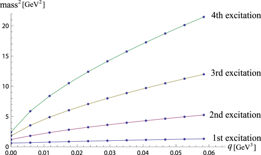
Figure 2: The first four excitations of the vector meson spectra.

3.2 Axial vector meson

We study the axial vector meson spectra. The axial vector can be decomposed into a transverse component and a longitudinal component as

$$a_{\scriptscriptstyle{M}}=\bar{a}_{\scriptscriptstyle{M}}+\partial_{\scriptscriptstyle{M}}\chi.$$ (3.17)

The $\bar{a}_{\scriptscriptstyle{M}}$ corresponds to the axial-vector meson. We choose the axial gauge, $\bar{a}_{\scriptscriptstyle{Z}}=0$. We consider the fluctuation fixing $\bar{a}_{\scriptscriptstyle{0}}=0$ as the Lorentz boost symmetry is not manifest. As the axial vector couples to the scalar field $v$ in the action (3.9) we solve the equation of motion for the scalar field as well. Under the dimension scale (3.12) the equation (3.6) becomes

$$\partial_{\tilde{z}}\left(\frac{f_{tc}}{\tilde{z}^{3}}e^{-\tilde{z}^{2}}\partial_{\tilde{z}}v\right)+\frac{3}{\tilde{z}^{5}}e^{-\tilde{z}^{2}}v=0.$$ (3.18)

The parameters in the scalar field (3.7) are scaled as

$$v=\tilde{m}_{q}\tilde{z}+\tilde{\sigma}\tilde{z}^{3}+\cdots,~{}~{}\tilde{m}_{q}=\frac{m_{q}}{\sqrt{c}},~{}~{}\tilde{\sigma}=\frac{\sigma}{c^{3/2}}.$$ (3.19)

By the Fourier transformed axial vector

$$\bar{a}_{i}(t,z)=\int\frac{d\omega}{2\pi}e^{-i\omega t}\tilde{\bar{a}}_{i}(\omega,z),$$ (3.20)

the equation of motion is obtained as

$$\partial_{z}\left(\frac{f_{tc}}{z}e^{-\Phi}\partial_{z}\tilde{\bar{a}}_{i}\right)-\frac{1}{z^{3}}e^{-\Phi}\left(g^{2}v^{2}-\frac{z^{2}}{f_{tc}}m_{\scriptscriptstyle{A}}^{2}\right)\tilde{\bar{a}}_{i}=0.$$ (3.21)

By the field redefinition $\tilde{\bar{a}}_{i}=e^{Y/2}\zeta_{i}$ with $Y=\tilde{z}^{2}-\log\frac{f_{tc}}{\tilde{z}}$, the equation (3.21) can be rewritten as

$${\zeta}^{\prime\prime}_{i}+\left(\frac{Y^{\prime\prime}}{2}-\frac{Y^{\prime 2}}{4}-\frac{1}{\tilde{z}^{2}f_{tc}}(g^{2}v^{2}-\frac{\tilde{z}^{2}}{f_{tc}}\tilde{m}_{\scriptscriptstyle{A}}^{2})\right)\zeta_{i}=0.$$ (3.22)

The mass spectra from the numerical solution of (3.18) and (3.21) for $m_{q}=0.005044\mathrm{GeV}$ and $\sigma=(0.2619\mathrm{GeV})^{3}$ are plotted in Fig 3. The meson mass increases as quark density increases.

$q(\mathrm{GeV}^{3})$	$n=0$	$n=1$	$n=2$	$n=3$
$0.0\times(0.388)^{3}$	$1.20195$	$2.04792$	$2.83813$	$3.59508$
$0.1\times(0.388)^{3}$	$1.20415$	$2.05663$	$2.85662$	$3.62591$
$0.2\times(0.388)^{3}$	$1.21044$	$2.08104$	$2.90742$	$3.70920$
$0.3\times(0.388)^{3}$	$1.21996$	$2.11703$	$2.98027$	$3.82575$
$0.4\times(0.388)^{3}$	$1.23155$	$2.15995$	$3.06494$	$3.95831$
$0.5\times(0.388)^{3}$	$1.24391$	$2.20579$	$3.15386$	$4.09546$
$0.6\times(0.388)^{3}$	$1.25581$	$2.25161$	$3.24237$	$4.23097$
$0.7\times(0.388)^{3}$	$1.26636$	$2.29591$	$3.32850$	$4.36251$
$0.8\times(0.388)^{3}$	$1.27537$	$2.33861$	$3.41222$	$4.49003$
$0.9\times(0.388)^{3}$	$1.28327$	$2.38044$	$3.49422$	$4.61415$
$1.0\times(0.388)^{3}$	$1.29080$	$2.42216$	$3.57504$	$4.73521$

Table 2: The first four excitations of the axial meson spectra in GeV for $m_{q}=0.005044\mathrm{GeV}$ and $\sigma=(0.2619\mathrm{GeV})^{3}$. $\sqrt{c}=0.388\mathrm{GeV}$.

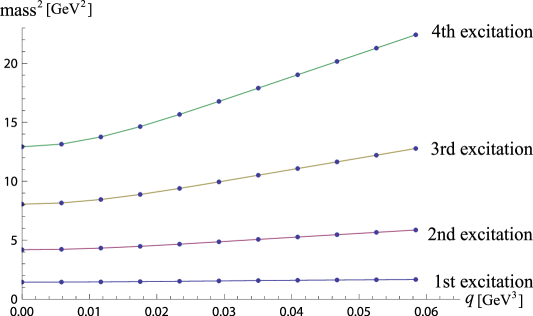
Figure 3: The first four excitations of the axial meson spectra for $m_{q}=0.005044\mathrm{GeV}$ and $\sigma=(0.2619\mathrm{GeV})^{3}$.

4 Discussion

We have studied the holographic QCD in hadronic medium by using the soft wall model, where the confinement scale is induced by a non-dynamical scalar field. We have observed the Hawking-Page transition between Reissner-Nordström AdS black hole and thermal charged AdS and obtained the phase diagram. The patterns of the plots at high chemical potentials are analogous to the diagrams of the hard wall model [28] whereas the patterns of the plots at low chemical potentials are distinguishable from the diagrams of the hard wall model. We have studied the vector and axial vector meson spectra depending on the quark density. In both cases the meson mass increases as quark density increases. The Regge behavior is not observed in the presence of the quark density.

We have discussed the model in the backgrounds of RNAdS BH and tcAdS whose geometries are not modified by the scalar field which induces the IR cutoff. It would be interesting to study relevant physical quantities in the geometry whose metric gets deformed by a scalar field. We will report those results elsewhere.

References

- [1] J. M. Maldacena, Adv. Theor. Math. Phys. 2, 231 (1998) [Int. J. Theor. Phys. 38, 1113 (1999)] [arXiv:hep-th/9711200]. S. S. Gubser, I. R. Klebanov and A. M. Polyakov, Phys. Lett. B 428, 105 (1998) [arXiv:hep-th/9802109]. E. Witten, Adv. Theor. Math. Phys. 2, 253 (1998) [arXiv:hep-th/9802150].
- [2] E. Witten, Adv. Theor. Math. Phys. 2, 505 (1998) [arXiv:hep-th/9803131].
- [3] J. Polchinski and M. J. Strassler, arXiv:hep-th/0003136.
- [4] I. R. Klebanov and M. J. Strassler, JHEP 0008, 052 (2000) [arXiv:hep-th/0007191].
- [5] J. M. Maldacena and C. Nunez, Phys. Rev. Lett. 86, 588 (2001) [arXiv:hep-th/0008001].
- [6] J. Polchinski and M. J. Strassler, Phys. Rev. Lett. 88, 031601 (2002) [arXiv:hep-th/0109174].
- [7] M. Kruczenski, D. Mateos, R. C. Myers and D. J. Winters, JHEP 0405, 041 (2004) [arXiv:hep-th/0311270].
- [8] T. Sakai and S. Sugimoto, Prog. Theor. Phys. 113, 843 (2005) [arXiv:hep-th/0412141]. T. Sakai and S. Sugimoto, Prog. Theor. Phys. 114, 1083 (2005) [arXiv:hep-th/0507073].
- [9] H. Boschi-Filho and N. R. F. Braga, JHEP 0305, 009 (2003) [arXiv:hep-th/0212207].
- [10] G. F. de Teramond and S. J. Brodsky, Phys. Rev. Lett. 94, 201601 (2005) [arXiv:hep-th/0501022].
- [11] J. Erlich, E. Katz, D. T. Son and M. A. Stephanov, Phys. Rev. Lett. 95, 261602 (2005) [arXiv:hep-ph/0501128].
- [12] L. Da Rold and A. Pomarol, Nucl. Phys. B 721, 79 (2005) [arXiv:hep-ph/0501218].
- [13] Y. Ko, B. H. Lee and C. Park, JHEP 1004, 037 (2010) [arXiv:0912.5274 [hep-ph]].
- [14] B. H. Lee, C. Park and S. Shin, JHEP 1012, 071 (2010) [arXiv:1010.1109 [hep-th]].
- [15] A. Karch, E. Katz, D. T. Son and M. A. Stephanov, Phys. Rev. D 74, 015005 (2006) [arXiv:hep-ph/0602229].
- [16] O. Andreev, Phys. Rev. D 73, 107901 (2006) [arXiv:hep-th/0603170]. O. Andreev and V. I. Zakharov, Phys. Rev. D 74, 025023 (2006) [arXiv:hep-ph/0604204]. O. Andreev and V. I. Zakharov, Phys. Rev. D 76, 047705 (2007) [arXiv:hep-ph/0703010].
- [17] H. Forkel, M. Beyer and T. Frederico, JHEP 0707, 077 (2007) [arXiv:0705.1857 [hep-ph]].
- [18] S. J. Brodsky and G. F. de Teramond, Phys. Lett. B 582, 211 (2004) [arXiv:hep-th/0310227]. S. J. Brodsky and G. F. de Teramond, Phys. Rev. Lett. 96, 201601 (2006) [arXiv:hep-ph/0602252]. S. J. Brodsky and G. F. de Teramond, Phys. Rev. D 77, 056007 (2008) [arXiv:0707.3859 [hep-ph]].
- [19] S. W. Hawking and D. N. Page, Commun. Math. Phys. 87, 577 (1983).
- [20] C. P. Herzog, Phys. Rev. Lett. 98, 091601 (2007) [arXiv:hep-th/0608151].
- [21] K. Y. Kim, S. J. Sin and I. Zahed, arXiv:hep-th/0608046.
- [22] N. Horigome and Y. Tanii, JHEP 0701, 072 (2007) [arXiv:hep-th/0608198].
- [23] S. Nakamura, Y. Seo, S. -J. Sin, K. P. Yogendran, J. Korean Phys. Soc. 52, 1734-1739 (2008). [hep-th/0611021].
- [24] S. Kobayashi, D. Mateos, S. Matsuura, R. C. Myers, R. M. Thomson, JHEP 0702, 016 (2007). [hep-th/0611099].
- [25] S. K. Domokos, J. A. Harvey, Phys. Rev. Lett. 99, 141602 (2007). [arXiv:0704.1604 [hep-ph]].
- [26] Y. Kim, B. -H. Lee, S. Nam, C. Park, S. -J. Sin, Phys. Rev. D76, 086003 (2007). [arXiv:0706.2525 [hep-ph]].
- [27] S. J. Sin, JHEP 0710, 078 (2007) [arXiv:0707.2719 [hep-th]].
- [28] B. H. Lee, C. Park and S. J. Sin, JHEP 0907, 087 (2009) [arXiv:0905.2800 [hep-th]].
- [29] C. Park, Phys. Rev. D 81, 045009 (2010) [arXiv:0907.0064 [hep-ph]].
- [30] K. Jo, B. -H. Lee, C. Park, S. -J. Sin, JHEP 1006, 022 (2010). [arXiv:0909.3914 [hep-ph]].
- [31] Y. Seo, J. P. Shock, S. J. Sin and D. Zoakos, JHEP 1003, 115 (2010) [arXiv:0912.4013 [hep-th]].
- [32] O. Andreev, Phys. Rev. D 81, 087901 (2010) [arXiv:1001.4414 [hep-ph]].
- [33] F. Bigazzi, A. L. Cotrone, J. Mas, D. Mayerson and J. Tarrio, JHEP 1104, 060 (2011) [arXiv:1101.3560 [hep-th]].
- [34] E. Witten, Adv. Theor. Math. Phys. 2, 253 (1998) [arXiv:hep-th/9802150].