Discussion of: A statistical analysis of multiple temperature proxies: Are reconstructions of surface temperatures over the last 1000 years reliable?

10.1214/10-AOAS398

Discussion on A statistical analysis of multiple temperature proxies: Are reconstructions of surface temperatures over the last 1000 years reliable? by B. B. McShane and A. J. Wyner

Lasse Holmstrom

This is an impressive paper. The authors present a thorough examination of the ability of various climate proxies to predict temperature. The prediction method is one much used in climate science literature and assumes a linear relationship between the proxies and the temperature. The idea is to use instrumental temperature data together with the corresponding proxy records to estimate a regression model to which historical proxy values are then input in order to produce a backcast of past temperature variation. The authors demonstrate convincingly that the data used in Mann et al. (2008) does not allow reliable temperature prediction using this approach and that purely random artificial proxy records, in fact, perform equally well or even better.

While this is certainly striking and thought-provoking, one should not be left under the impression that this is the standard approach to understanding past climate and that temperature reconstruction per se is impossible. In fact, some of the “proxies” used in the paper are themselves supposedly successful temperature reconstructions and therefore arguably of a more fundamental character than the predictor produced by the Lasso. There is, for example, a long and well-established paleoecological tradition of quantitative environmental reconstruction based on diatoms, pollen, chironomids and other biological proxies that in some important aspects differs from the regression approach used in the present paper and that can offer better prediction accuracy [e.g., Birks (1995); Birks et al. (2010)]. A typical temperature reconstruction in this tradition uses a sediment core from a selected lake together with training data from a number of other lakes to backcast temperatures hundreds or thousands of years in time. As a proxy one can use the relative abundances of various organisms (say, different diatom taxa) measured at various depths along the core. A model for the dependence between the temperature and the abundances is built using a training set that consists of the relative abundances of the same the same organisms in surface sediment samples from a large number of lakes located in the same general area as the core lake and their current temperatures, mean July temperature being a typical climate variable. The training lakes are selected to cover a wide range of environmental conditions to make possible temperature backcasting to times when the conditions at the core lake possibly were very different from what they are today. This is referred to as space-for-time substitution.

Compared to the approach studied in this paper, at least two differences seem clear: the relative locality of the analysis and the possibility in some cases to incorporate ecological information in the model. Instead of a global proxy network, this method typically uses local proxy data to backcast local environmental conditions. Ecological information can enter the model, for example, through a hierarchical model component that explicitly incorporates the fact that different organisms have different optimal temperatures, that is, temperatures at which they fare particularly well. Various models, including methods based on parametric or nonparametric regression, as well Bayesian approaches, have been proposed. Such reconstructions appear to quite successfully capture many large-scale Holocene climate features such as the Medieval Warm Period and the Little Ice Age. I wonder if the rather strict locality of the approach combined with at least some degree of ecological plausibility in modeling the proxy data generating process are factors in their apparent success?

Recently, Bayesian approaches have begun to enter the field. The first papers that used detailed Bayesian modeling for paleoclimate reconstruction were Vasko, Toivonen and Korhola (2000), Toivonen et al. (2001) and Korhola et al. (2002). More recently, Haslett et al. (2006) and Erästö and Holmström (2006) have taken similar approaches. As reconstruction in the Bayesian setting produces the posterior distribution of the past temperature variation, such important questions as joint (pathwise) credibility of past temperature features also discussed in the present paper can be easily answered.

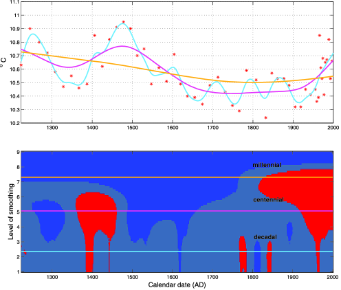
Figure 1: Scale space analysis of the salient features of a diatom-based temperature reconstruction in Northern Fennoscandia for the past 800 years. Upper panel: the reconstructed temperatures (asterisks) together with three smooths. Lower panel: scale space credibility map with the horizontal lines indicating the corresponding three levels of smoothing. For more details, see Weckström et al. (2006) and the text. Code and data to reproduce this figure can be found in the supplementary file to this discussion.

Another question I would like to consider is the possible role of smoothing, briefly touched upon at the end of Section 3. As pointed out by the authors, one difficulty is the choice of a proper smoothing level. However, in the so-called scale space approach this difficulty is turned into an opportunity when, instead of just one, in some sense optimal smooth, one considers a whole family of smooths. Our paleoecologist collaborators have found quite useful a procedure where such multi-level smoothing is applied to the reconstructed temperature time series. Each smooth can then be interpreted to provide information about the underlying past temperature variation at a particular time scale, little smoothing showing the short time scale details and heavy smoothing leaving only the coarsest features, such as the overall trend. For a Bayesian reconstruction, such scale space smoothing can easily be combined with a credibility analysis of these multi-scale features, but similar analyses are possible also in a non-Bayesian setting [e.g., Erästö and Holmström (2005, 2006, 2007); Holmström and Erästö (2002); Korhola et al. (2000); Godtliebsen, Olsen and Winther (2003); Rohling and Pälike (2005)].

It is also possible to combine a non-Bayesian reconstruction with Bayesian scale space analysis. This is useful as the vast majority of existing paleoreconstructions are non-Bayesian. Thus, suppose that $\mu(t_{i})$ is the true past temperature at time $t_{i}$, $i=1,\ldots,n$, and let $y_{i}=\mu(t_{i})+\varepsilon_{i}$ be its reconstructed value. After specifying pri- ors for $\mu$ and the reconstruction errors $\varepsilon_{i}$ the posterior distribution $p(\mu^{\prime}|y_{1},\ldots,y_{n})$ of the derivative of $\mu$ can then be obtained. The scale space analysis now consists of smoothing this posterior at different levels in order to find the credible features of past temperature variation in different scales. It is also possible to handle correlated errors as well as errors in the time points $t_{i}$. For details see Erästö and Holmström (2005, 2007).

An example of this idea is shown in Figure 1, where an analysis of a diatom-based temperature reconstruction in Northern Fennoscandia for the past 800 years is shown. In the upper panel, asterisks show the actual reconstructed temperatures together with three smooths (posterior means) reflecting variation in millennial, centennial and decadal timescales. The lower panel map summarizes the scale space inference. Following any horizontal line in this map we see when, at that particular smoothing level, or time scale, the local temperature trend has been credibly positive (red) or negative (blue) or when no credible change has occurred (gray). Inference is joint over all time points. In this analysis, the Little Ice Age shows as a credible broad minimum in several different scales, from century to millennial scales (the color changing from blue to red), whereas the overall millennial trend has been negative. The very recent warming after industrialization shows as red in many scales.

Supplement [doi]10.1214/10-AOAS398HSUPP [url]http://lib.stat.cmu.edu/aoas/398H/supplementH.zip .zip Code and data to reproduce Figure 1 can be found in the supplementary files to this discussion.

References

- Birks (1995) {bmisc}[auto:STB—2010-11-18—09:18:59] \bauthor\bsnmBirks, \bfnmH. J. B.\binitsH. J. B. (\byear1995). \bhowpublishedQuantitative palaeoenvironmental reconstructions. In Statistical Modelling of Quaternary Science Data (D. Maddy and J. S. Brew, eds.). Technical Guide 5 161–254. Quaternary Research Association, Cambridge. \endbibitem
- Birks et al. (2010) {bmisc}[auto:STB—2010-11-18—09:18:59] \bauthor\bsnmBirks, \bfnmH. J. B.\binitsH. J. B., \bauthor\bsnmHeiri, \bfnmO.\binitsO., \bauthor\bsnmSeppä, \bfnmH.\binitsH. and \bauthor\bsnmBjune, \bfnmA. E.\binitsA. E. (\byear2010). \bhowpublishedStrengths and weaknesses of quantitative climate reconstructions based on late-quaternary biological proxies. Unpublished manuscript. \endbibitem
- Erästö and Holmström (2005) {barticle}[mr] \bauthor\bsnmErästö, \bfnmPanu\binitsP. and \bauthor\bsnmHolmström, \bfnmLasse\binitsL. (\byear2005). \btitleBayesian multiscale smoothing for making inferences about features in scatterplots. \bjournalJ. Comput. Graph. Statist. \bvolume14 \bpages569–589. \biddoi=10.1198/106186005X59315, mr=2170202 \endbibitem
- Erästö and Holmström (2006) {barticle}[auto:STB—2010-11-18—09:18:59] \bauthor\bsnmErästö, \bfnmP.\binitsP. and \bauthor\bsnmHolmström, \bfnmL.\binitsL. (\byear2006). \btitlePrior selection and multiscale analysis in Bayesian temperature reconstruction based on species assemblages. \bjournalJournal of Paleolimnology \bvolume36 \bpages69–80. \endbibitem
- Erästö and Holmström (2007) {barticle}[mr] \bauthor\bsnmErästö, \bfnmPanu\binitsP. and \bauthor\bsnmHolmström, \bfnmLasse\binitsL. (\byear2007). \btitleBayesian analysis of features in a scatter plot with dependent observations and errors in predictors. \bjournalJ. Stat. Comput. Simul. \bvolume77 \bpages421–434. \biddoi=10.1080/10629360600711988, mr=2395958 \endbibitem
- Godtliebsen, Olsen and Winther (2003) {barticle}[auto:STB—2010-11-18—09:18:59] \bauthor\bsnmGodtliebsen, \bfnmF.\binitsF., \bauthor\bsnmOlsen, \bfnmL. R.\binitsL. R. and \bauthor\bsnmWinther, \bfnmJ. G.\binitsJ. G. (\byear2003). \btitleRecent developments in statistical time series analysis: Examples of use in climate research. \bjournalGeophysical Research Letters \bnote1654. doi:10.1029/2003GL017229. \endbibitem
- Haslett et al. (2006) {barticle}[mr] \bauthor\bsnmHaslett, \bfnmJ.\binitsJ., \bauthor\bsnmWhiley, \bfnmM.\binitsM., \bauthor\bsnmBhattacharya, \bfnmS.\binitsS., \bauthor\bsnmSalter-Townshend, \bfnmM.\binitsM., \bauthor\bsnmWilson, \bfnmSimon P.\binitsS. P., \bauthor\bsnmAllen, \bfnmJ. R. M.\binitsJ. R. M., \bauthor\bsnmHuntley, \bfnmB.\binitsB. and \bauthor\bsnmMitchell, \bfnmF. J. G.\binitsF. J. G. (\byear2006). \btitleBayesian palaeoclimate reconstruction. \bjournalJ. Roy. Statist. Soc. Ser. A \bvolume169 \bpages395–438. \biddoi=10.1111/j.1467-985X.2006.00429.x, mr=2236914 \endbibitem
- Holmström and Erästö (2002) {barticle}[mr] \bauthor\bsnmHolmström, \bfnmLasse\binitsL. and \bauthor\bsnmErästö, \bfnmPanu\binitsP. (\byear2002). \btitleMaking inferences about past environmental change using smoothing in multiple time scales. \bjournalComput. Statist. Data Anal. \bvolume41 \bpages289–309. \biddoi=10.1016/S0167-9473(02)00079-8, mr=1945872 \endbibitem
- Korhola et al. (2000) {barticle}[auto:STB—2010-11-18—09:18:59] \bauthor\bsnmKorhola, \bfnmA.\binitsA., \bauthor\bsnmWeckström, \bfnmJ.\binitsJ., \bauthor\bsnmHolmström, \bfnmL.\binitsL. and \bauthor\bsnmErästö, \bfnmP.\binitsP. (\byear2000). \btitleA quantitative Holocene climatic record from diatoms in northern Fennoscandia. \bjournalQuaternary Research \bvolume54 \bpages284–294. \endbibitem
- Korhola et al. (2002) {barticle}[auto:STB—2010-11-18—09:18:59] \bauthor\bsnmKorhola, \bfnmA.\binitsA., \bauthor\bsnmVasko, \bfnmK.\binitsK., \bauthor\bsnmToivonen, \bfnmH. T. T.\binitsH. T. T. and \bauthor\bsnmOlander, \bfnmH.\binitsH. (\byear2002). \btitleHolocene temperature changes in northern Fennoscandia reconstructed from chironomids using Bayesian modelling. \bjournalQaternary Science Reviews \bvolume21 \bpages1841–1860. \endbibitem
- Mann et al. (2008) {barticle}[auto:STB—2010-11-18—09:18:59] \bauthor\bsnmMann, \bfnmM. E.\binitsM. E., \bauthor\bsnmZhang, \bfnmZ.\binitsZ., \bauthor\bsnmHughes, \bfnmM. K.\binitsM. K., \bauthor\bsnmBradley, \bfnmR. S.\binitsR. S., \bauthor\bsnmMiller, \bfnmS. K.\binitsS. K., \bauthor\bsnmRutherford, \bfnmS.\binitsS. and \bauthor\bsnmNi, \bfnmF.\binitsF. (\byear2008). \btitleProxy-based reconstructions of hemispheric and global surface temperature variations over the past two millenia. \bjournalProc. Natl. Acad. Sci. USA \bvolume105 \bpages36. \endbibitem
- Rohling and Pälike (2005) {barticle}[pbm] \bauthor\bsnmRohling, \bfnmEelco J.\binitsE. J. and \bauthor\bsnmPälike, \bfnmHeiko\binitsH. (\byear2005). \btitleCentennial-scale climate cooling with a sudden cold event around 8,200 years ago. \bjournalNature \bvolume434 \bpages975–979. \bidpii=nature03421, doi=10.1038/nature03421, pmid=15846336 \endbibitem
- Toivonen et al. (2001) {barticle}[auto:STB—2010-11-18—09:18:59] \bauthor\bsnmToivonen, \bfnmH. T. T.\binitsH. T. T., \bauthor\bsnmMannila, \bfnmH.\binitsH., \bauthor\bsnmKorhola, \bfnmA.\binitsA. and \bauthor\bsnmOlander, \bfnmH.\binitsH. (\byear2001). \btitleApplying Bayesian statistics to organism-based environmental reconstruction. \bjournalEcological Applications \bvolume11 \bpages618–630. \endbibitem
- Vasko, Toivonen and Korhola (2000) {barticle}[auto:STB—2010-11-18—09:18:59] \bauthor\bsnmVasko, \bfnmK.\binitsK., \bauthor\bsnmToivonen, \bfnmH. T.\binitsH. T. and \bauthor\bsnmKorhola, \bfnmA.\binitsA. (\byear2000). \btitleA Bayesian multinomial Gaussian response model for organism-based environmental reconstruction. \bjournalJournal of Paleolimnology \bvolume24 \bpages243–250. \endbibitem
- Weckström et al. (2006) {barticle}[auto:STB—2010-11-18—09:18:59] \bauthor\bsnmWeckström, \bfnmJ.\binitsJ., \bauthor\bsnmKorhola, \bfnmA.\binitsA., \bauthor\bsnmErästö, \bfnmP.\binitsP. and \bauthor\bsnmHolmström, \bfnmL.\binitsL. (\byear2006). \btitleTemperature patterns over the past eight centuries in Northern Fennoscandia inferred from sedimentary diatoms. \bjournalQuaternary Research \bvolume66 \bpages78–86. \endbibitem