Spurious predictions with random time series: The Lasso in the context of paleoclimatic reconstructions. Discussion of: A statistical analysis of multiple temperature proxies: Are reconstructions of surface temperatures over the last 1000 years reliable?

10.1214/10-AOAS398

Discussion on A statistical analysis of multiple temperature proxies: Are reconstructions of surface temperatures over the last 1000 years reliable? by B. B. McShane and A. J. Wyner

a1A more detailed version of this discussion is available at http://people.fas.harvard.edu/ ~tingley/.

Blakeley B. McShane and Abraham J. Wyner (hereafter, MW2011) find that, under certain scenarios and using the LASSO to fit regression models, randomly generated series are as predictive of past climate as the commonly used proxies (MW2011, Figure 9). They conclude that “the proxies do not predict temperature significantly better than random series generated independently of temperature,” a claim that has already been reproduced in the popular press (The Wall Street Journal, 2010). If this assertion is correct, then MW2011 have undermined all efforts to reconstruct past climate, which are based on the fundamental assumption that natural proxies are predictive of past climate. I disagree with MW2011’s conclusion and provide an alternative explanation: the LASSO, as applied in MW2011, is simply not an appropriate tool for reconstructing paleoclimate.

To shed light on the MW2011 results, I turn to an experiment with surrogate data (Tingley, 2011). The “target” time series, analogous to the Northern Hemisphere mean temperature time series in MW2011, is the sum of a simple linear trend and an AR(1) process, $y(t)=0.25\cdot t+\varepsilon(t),t=1,\ldots,149$. The AR(1) coefficient in the $\varepsilon$ process is $0.4$, and the variance of the innovations is 1. I then generate 1138 “pseudo-proxy” time series by adding white noise to this target series. The signal to noise ratio (SNR) of these pseudo-proxies, expressed as the ratio of the standard deviation of the target time series to that of the additive white noise, will take on a range of values $(4,2,1,1/2,1/4,1/8)$. In order to compare the performance of these pseudo-proxies to random series, I generate 1138 independent AR(1) time series, each of length 149; the common AR(1) coefficient, $\alpha$, for these random series will take on a range of values (0, 0.2, 0.4, 0.6, 0.8, 1.0). Two regression models are then fit using 119 of the 149 observations.

The first model, referred to as “composite regression,” involves averaging across all predictor series and then using this composite series to predict the target via ordinary least squares regression. The second model applies the LASSO to all predictor series, and is fit using the algorithm described in Friedman et al. (2007, 2010) and the glmnet package for Matlab (available at http://www-stat.stanford.edu/~tibs/glmnet-matlab/). The LASSO penalization parameter ($\lambda$ on page 13 of MW2011) is set to be 0.05 times the smallest value of $\lambda$ for which all coefficients are zero; the LASSO penalization is thus very small.

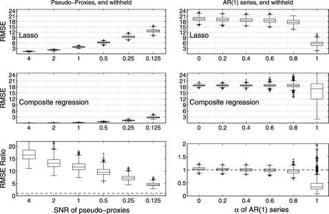
Figure 1: Out-of-sample RMSE calculated using 30 values withheld from the end of each surrogate data set. Left column: using pseudo-proxies as predictors. Right column: using independent AR(1) series as predictors. Top row: regression using the LASSO. Middle row: composite regression. Bottom row: the ratio of the LASSO RMSE value to the composite regression RMSE.

Box plots of the out-of-sample RMSE are shown in Figure 1 for 1000 experiments that calculate the RMSE using observations withheld from the end of the data set; results are similar when observations are withheld from the interior. Composite regression results in lower RMSE than the LASSO for all values of the pseudo-proxy SNR (Figure 1, left column). For an SNR of $1/4$, the LASSO RMSE is about 7.5 times larger than the composite regression RMSE. This is a clear indication that the LASSO is not making effective use of the information contained in the pseudo-proxies.

Applying the LASSO to AR(1) series with sufficiently high $\alpha$ values results in lower out-of-sample RMSE values than applying the LASSO to the noisier pseudo-proxies (compare the two top panels of Figure 1). This is the result discussed in MW2011: the LASSO gives better results when applied to highly structured random time series than when applied to noisy predictors that do in fact contain information about the target series. Note in addition that for values of $\alpha\geq 0.8$, the LASSO on the AR(1) series results in lower RMSE than using composite regression on AR(1) series with $\alpha=0$ (the limiting case of an SNR of zero for the pseudo-proxies). These results can be explained by the structure of the surrogate data experiment, which sets the target series to be linear in time, with additive AR(1) noise. The LASSO applied to AR(1) series with $\alpha=1$ results in nonzero coefficients for only those predictor series that display strong, linear trends over the calibration interval, and the expected value of a predictor series during the validation interval is then the last value in the calibration interval. In contrast, as the SNR${}\rightarrow 0$, composite regression on the pseudo-proxies approaches (in expectation) the intercept model. These features are illustrated in Figure 2.

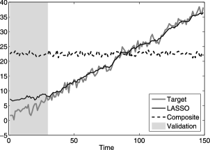
Figure 2: Example fits from applying the LASSO to random walk predictors and composite regression to white noise predictors. Shading indicates the portion of the data set withheld for validation.

MW2011 point out that highly structured random series (large $\alpha$) are well suited to interpolation, and to a lesser extent extrapolation, on short time scales. As the variance of the white noise component of the pseudo-proxies increases, these predictors become both less informative of the target series, and less structured in time. At a certain SNR, short-term interpolations or extrapolations based on independent, but more temporally structured series, perform better. This threshold SNR is a decreasing function of the length of the extrapolation/interpolation interval. As the goal in a paleoclimate context is extrapolation on long timescales, composite regression on extraordinarily noisy proxies will outperform the LASSO applied to random walks.

The LASSO gives inferior results in situations where each of a large number of predictors is only weakly correlated with the target series, but the mean across all predictors is highly correlated with that target. It is well known that the LASSO is the posterior mode which results from placing a common double exponential prior on the regression coefficients [Park and Casella (2008)]. It is difficult to imagine a scientifically defensible reason for specifying such a prior in the paleoclimate context. A more scientifically reasonable approach is to modify the LASSO prior to shrink the regression coefficients not towards zero, but toward a common, data determined value. Such a prior reflects the assumptions that (1) the regression coefficients are likely to be similar to one another, and (2) all predictors are informative of the target series. Within the paleoclimate context, where the expectation is that each proxy is weakly correlated to the northern hemisphere mean (for two reasons: proxies generally have a weak correlation with local climate, which in turn is weakly correlated with a hemispheric average) the LASSO as used by MW2011 is simply not an appropriate tool. It throws away too much information.

More generally, MW2011 have perhaps missed a larger point. The presence of a large number of correlated predictors is intrinsic to the paleoclimate reconstruction problem and has a geophysical basis. MW2011 state that, “it is unavoidable that some type of dimensionality reduction is necessary, even if there is no principled way to achieve this.” This is simply not the case. A more scientifically sound approach recognizes that the proxies are related to the local climate, which in turn displays both spatial and temporal correlation. These ideas can be encoded in hierarchical statistical models, which can combine the specification of a parametric spatiotemporal covariance form for the target climate process (e.g., surface temperature anomalies) with reasonable forward models that describe the conditional distribution of the proxy observations given the climate process. Such approaches naturally account for the $p\gg n$ problem, and for the strong correlations between the proxies. These models are derived from the rich development of Bayesian statistics over the past 20 years and are being adapted by the paleoclimate community. See Tingley and Huybers (2010) for a specific example, and Tingley et al. (2010) for a comprehensive discussion.

References

- Friedman, Hastie and Tibshirani (2010) {barticle}[auto:STB—2010-11-18—09:18:59] \bauthor\bsnmFriedman, \bfnmJ.\binitsJ., \bauthor\bsnmHastie, \bfnmT.\binitsT. and \bauthor\bsnmTibshirani, \bfnmR.\binitsR. (\byear2010). \btitleRegularization paths for generalized linear models via coordinate descent. \bjournalJournal of Statistical Software \bvolume33 \bpages1–22. \endbibitem
- Friedman et al. (2007) {barticle}[mr] \bauthor\bsnmFriedman, \bfnmJerome\binitsJ., \bauthor\bsnmHastie, \bfnmTrevor\binitsT., \bauthor\bsnmHöfling, \bfnmHolger\binitsH. and \bauthor\bsnmTibshirani, \bfnmRobert\binitsR. (\byear2007). \btitlePathwise coordinate optimization. \bjournalAnn. Appl. Statist. \bvolume1 \bpages302–332. \biddoi=10.1214/07-AOAS131, mr=2415737 \endbibitem
- Park and Casella (2008) {barticle}[mr] \bauthor\bsnmPark, \bfnmTrevor\binitsT. and \bauthor\bsnmCasella, \bfnmGeorge\binitsG. (\byear2008). \btitleThe Bayesian Lasso. \bjournalJ. Amer. Statist. Assoc. \bvolume103 \bpages681–686. \biddoi=10.1198/016214508000000337, mr=2524001 \endbibitem
- The Wall Street Journal (2010) {bmisc}[auto:STB—2010-11-18—09:18:59] \borganizationThe Wall Street Journal (\byear2010). \bhowpublishedEditorial: Climate of uncertainty, 02 September 2010. Available at http://online.wsj.com/article/SB10001424052748703467004575463433671739148.html. \endbibitem
- Tingley (2011) {bmisc}[auto:STB—2010-11-18—09:18:59] \bauthor\bsnmTingley, \bfnmM. P.\binitsM. P. (\byear2011). \bhowpublishedSupplement to “Spurious predictions with random time series: The Lasso in the context of paleoclimatic reconstructions. Discussion of: A statistical analysis of multiple temperature proxies: Are reconstructions of surface temperatures over the last 1000 years reliable?” DOI: 10.1214/10-AOAS398ESUPP. \endbibitem
- Tingley and Huybers (2010) {barticle}[auto:STB—2010-11-18—09:18:59] \bauthor\bsnmTingley, \bfnmM. P.\binitsM. P. and \bauthor\bsnmHuybers, \bfnmP.\binitsP. (\byear2010). \btitleA Bayesian algorithm for reconstructing climate anomalies in space and time. Part 1: Development and applications to paleoclimate reconstruction problems. \bjournalJournal of Climate \bvolume23 \bpages2759–2781. \endbibitem
- Tingley et al. (2010) {bmisc}[auto:STB—2010-11-18—09:18:59] \bauthor\bsnmTingley, \bfnmM. P.\binitsM. P., \bauthor\bsnmCraigmile, \bfnmP. F.\binitsP. F., \bauthor\bsnmHaran, \bfnmM.\binitsM., \bauthor\bsnmLi, \bfnmB.\binitsB., \bauthor\bsnmMannshardt-Shamseldin, \bfnmE.\binitsE. and \bauthor\bsnmRajaratnam, \bfnmB.\binitsB. (\byear2010). \bhowpublishedPiecing together the past: Statistical insights into paleoclimatic reconstructions. Technical Report 2010–09. Dept. Statistics, Stanford Univ. Available at http://statistics.stanford.edu/~ckirby/reports/2010_2019/reports2010.html. \endbibitem