Computer Algebra meets Finite Elements: an Efficient Implementation for Maxwell’s Equations

Abstract

We consider the numerical discretization of the time-domain Maxwell’s equations with an energy-conserving discontinuous Galerkin finite element formulation. This particular formulation allows for higher order approximations of the electric and magnetic field. Special emphasis is placed on an efficient implementation which is achieved by taking advantage of recurrence properties and the tensor-product structure of the chosen shape functions. These recurrences have been derived symbolically with computer algebra methods reminiscent of the holonomic systems approach.

1 Introduction

This paper is dedicated to a successful cooperation between symbolic computation and numerical analysis. The goal is to simulate the propagation of electromagnetic waves using finite element methods (FEM). Such simulations play an important role for constructing antennas, electric circuit boards, bodyworks, and many other devices where electromagnetic radiation is involved. The numerical simulation of such physical phenomena helps to optimize the shape of components and saves the engineer from doing a long and expensive series of experiments.

Finite element methods serve to approximate the solution of partial differential equations on a given domain $\Omega\subseteq\mathbbm{R}^{d}$ subject to certain constraints (e.g., boundary conditions). The domain $\Omega$ is partitioned into small elements (typically triangles or tetrahedra) and the solution is approximated on each element by means of certain shape functions. In our application we deal with Maxwell’s equations which relate the magnetic and the electric field. In Section 2 we describe how the problem can be discretized using FEM and in Section 3 we give the details concerning an efficient implementation.

An important ingredient for the fast execution of some operations in the FEM are certain difference-differential relations that were derived with computer algebra methods. The methods that we employ, originate in Zeilberger’s holonomic systems approach [13, 3, 10] whose basic idea is to define functions and sequences in terms of differential equations and recurrence equations plus initial values (these equations have to be linear with polynomial coefficients). Luckily the shape functions used in the chosen FEM discretization fit into the holonomic framework since they are defined in terms of orthogonal polynomials. Section 4 explains how the desired relations have been computed.

2 FEM formulation of Maxwell’s equations

In order to describe electromagnetic wave propagation problems, we consider the loss-free time-domain Maxwell’s equations

$$\varepsilon\frac{\partial E}{\partial t} = \operatorname{curl}H,$$

$$\mu\frac{\partial H}{\partial t} = -\operatorname{curl}E,$$

subject to appropriate initial and boundary conditions. Here $E=E(x,t)$ denotes the electric and $H=H(x,t)$ the magnetic field strength (with $x=(x_{1},x_{2},x_{3})$ the space variables and $t$ the time), and $\varepsilon$ and $\mu>0$ are the permittivity and the permeability, respectively. When discretizing these equations with the finite element method, we go over to a weak formulation by multiplying both equations with test functions $e(x)$ and $h(x)$ and integrating over the whole domain $\Omega\subset\mathbbm{R}^{3}$. The solution of the Maxwell’s equations then has to fulfill the conditions

$$\begin{array}[]{rcl}\displaystyle\frac{\partial}{\partial t}(\varepsilon E,e)_{\Omega}&=&(\operatorname{curl}H,e)_{\Omega},\\[8.61108pt] \displaystyle\frac{\partial}{\partial t}(\mu H,h)_{\Omega}&=&-(\operatorname{curl}E,h)_{\Omega}\end{array}$$ (1)

for all test functions $e$ and $h$, where $(\cdot,\cdot)_{\Omega}$ is the short notation for the $L^{2}(\Omega)$ inner product $(a,b)_{\Omega}=\int_{\Omega}ab\,\mathrm{d}x$. Then we replace both the magnetic and electric field as well as the test functions by finite-dimensional approximations on a triangulation $\mathcal{T}_{h}$ of the domain $\Omega$. Herein $h$ denotes some characteristic length of the elements in $\mathcal{T}_{h}$ (not to be confused with the test function $h$).

Conforming finite elements ensure that the finite-dimensional approximations are within a space which is appropriate for the partial differential equations under consideration. For Maxwell’s equations this space is $H(\operatorname{curl},\Omega)$ which demands tangential components to be continuous across element interfaces. The discontinuous Galerkin finite element method (DG) neglects this conformity condition when building up a discrete basis for the approximation, but instead has to incorporate stabilization terms to achieve a consistent and stable formulation. This is normally done by applying integration by parts and replacing fluxes at element boundaries with numerical fluxes [1, 11, 8, 7]. The latter approach has the major advantage that the mass matrices $M_{\varepsilon}$ and $M_{\mu}$, i.e., the matrices that arise when discretizing $(\varepsilon E,e)_{\Omega}$ and $(\mu H,h)_{\Omega}$, respectively, are block-diagonal which makes the application of their inverses computationally more efficient.

We consider the approximation space

$$V_{h}^{k}=\left\{v\in\left(L^{2}(\Omega)\right)^{3}:v|_{T}\in\left(\mathcal{P}^{k}(T)\right)^{3}\ \forall T\in\mathcal{T}_{h}\right\}$$

that consists of functions which are piecewise polynomial up to degree $k$. By integration by parts of (1) on each element $T\in\mathcal{T}_{h}$, and by adding a consistent stabilization term on all element boundaries we get (again for all test functions $e$ and $h$)

$$\frac{\partial}{\partial t}\sum_{T\in\mathcal{T}_{h}}(\varepsilon E,e)_{T} = \sum_{T\in\mathcal{T}_{h}}\big{(}(H,\operatorname{curl}e)_{T}+(H^{*}\times\nu,e)_{\partial T}\big{)},$$

$$\frac{\partial}{\partial t}\sum_{T\in\mathcal{T}_{h}}(\mu H,h)_{T} = \sum_{T\in\mathcal{T}_{h}}\big{(}-(\operatorname{curl}{E},h)_{T}+(E^{*}-E,h\times\nu)_{\partial T}\big{)},$$

where $\nu$ denotes the outer normal on each element boundary and $H^{*}$, $E^{*}$ are the numerical fluxes. The properties of different DG formulations mainly depend on the choice of the numerical fluxes. As all derivatives are now shifted to the electric field $E$ and the according test functions $e$, it is reasonable to approximate the electric field of one degree higher than the magnetic field. So we choose the approximation spaces $V_{h}^{k+1}$ for $E$ and $e$ and $V_{h}^{k}$ for $H$ and $h$.

2.1 Numerical flux

Several choices for the numerical flux are used in practice. Our goal here is to derive a numerical flux which ensures that the numerical approximation fulfills the following two important properties which are already fulfilled on the continuous level:

1. conservation of the energy $\frac{1}{2}(\varepsilon E,E)_{\Omega}+\frac{1}{2}(\mu H,H)_{\Omega}$

2. non-existence of spurious modes

On the one hand using dissipative fluxes avoids spurious modes and is often used, but as it introduces dissipation, the energy of the system is not conserved. On the other hand the standard approach for energy conserving methods is the so called central flux. Its mayor disadvantage is, that it introduces non-physical modes, spurious modes.

Nevertheless we start with this approach to derive the stabilized central flux formulation which gets rid of both problems. A more extensive discussion of numerical fluxes (including the stabilized central flux) for Maxwell’s equations can be found in [6, 8.2].

The central flux takes the averaged values of neighboring elements for the numerical flux, i.e., $H^{*}=\{\!\!\{H\}\!\!\}$ and $E^{*}=\{\!\!\{E\}\!\!\}$ with $\{\!\!\{\cdot\}\!\!\}$ denoting the averaging operator, and ends up with a semi-discrete system of the form

$$\frac{\partial}{\partial t}\begin{pmatrix}M_{\varepsilon}&\\ &M_{\mu}\end{pmatrix}\begin{pmatrix}E\\ H\end{pmatrix}=\begin{pmatrix}&-C_{h}^{T}\\ C_{h}&\end{pmatrix}\begin{pmatrix}E\\ H\end{pmatrix}$$ (2)

where $C_{h}$ denotes the discrete $\operatorname{curl}$ operator stemming from the central flux formulation. The matrix on the left side is symmetric and positive definite whereas the matrix on the right side is antisymmetric. Then the evolution matrix for the modified unknowns $(M_{\varepsilon}^{\frac{1}{2}}E,M_{\mu}^{\frac{1}{2}}H)^{T}$ is also antisymmetric and thus the proposed energy is conserved. Nevertheless this matrix has a lot of eigenvalues close to zero which correspond to the discretization, but not to the physical behavior of the system. To motivate the modification which will stabilize the formulation, let us have a brief look at the problem in frequency domain, i.e., for time-harmonic electric and magnetic fields. Then the discrete problem in frequency domain reads (with frequency $\omega$):

$$0=(i\omega)^{2}(M_{\varepsilon}E,e)+(M_{\mu}^{-1}C_{h}E,C_{h}e).$$ (3)

The problem with non-physical zero eigenvalues now manifests in $(C_{h}E,C_{h}e)$ being only positive semidefinite. We overcome this issue by adding a stabilization bilinear form $S(E,e)$ to (3) as proposed in [6].

$$S(E,e):=\sum_{F\in\mathcal{F}_{h}}\frac{\alpha}{h}([\![E]\!]\times\nu,[\![e]\!]\times\nu)_{F}$$

with $\alpha>0$, where $\mathcal{F}_{h}$ is the union of all element boundaries and $[\![\cdot]\!]$ denotes the jump operator, i.e., the difference between values of adjacent elements. This stabilization bilinearform eliminates the nontrivial kernel of $C_{h}$ and is consistent as $[\![E]\!]\times\nu$ is zero for the exact solution. Before we can translate the formulation back to the time domain, we introduce a new variable which is defined as

$$H^{F}:=\frac{([\![E]\!]\times\nu)\alpha}{i\omega h}$$

The new unknown $H^{F}$ is also piecewise polynomial on each face.

If we go back to the time-domain formulation we end up with the following formulation (note that relations between $[\![\cdot]\!]$ and $\{\!\!\{\cdot\}\!\!\}$ were used):

$$\frac{\partial}{\partial t}\sum_{T\in\mathcal{T}_{h}}(\varepsilon E,e)_{T} = \sum_{T\in\mathcal{T}_{h}}\big{(}(H,\operatorname{curl}e)_{T}+(\{\!\!\{H\}\!\!\}\times\nu,e)_{\partial T}\big{)}+$$

$$\sum_{F\in\mathcal{F}_{h}}(H^{F}\times\nu,[\![e]\!])_{F},$$

$$\frac{\partial}{\partial t}\sum_{T\in\mathcal{T}_{h}}(\mu H,h)_{T} = \sum_{T\in\mathcal{T}_{h}}\big{(}-(h,\operatorname{curl}E)_{T}+(\textstyle\frac{1}{2}[\![E]\!]\times\nu,h)_{\partial T}\big{)},$$

$$\frac{\partial}{\partial t}\sum_{F\in\mathcal{F}_{h}}\frac{\alpha}{h}(H^{F},h^{F})_{F} = \sum_{F\in\mathcal{F}_{h}}([\![E]\!]\times\nu,h^{F})_{F}.$$

For $p$-robust behavior $\alpha$ should scale with $p^{2}$, where $p$ is the polynomial degree. This is motivated by the symmetric interior penalty method for elliptic equations (see e.g. [1]) where a scaling of $\alpha$ with $p^{2}$ in the bilinearform $S$ is necessary for stability to dominate over some terms stemming from inverse inequalities which scale with $p^{2}$ (see also [7]).

We again achieve a system of the form (2) where the vector $H$ now consists of element and face unknowns and the matrix representing the discrete $\operatorname{curl}$ operator is the stabilized central flux $\operatorname{curl}$ operator now. Thus we conclude that the method now conserves energy, and spurious modes, introduced by the central flux, vanish.

2.2 Numerical Examples (Spherical Vacuum Resonator)

We consider a spherical domain $\Omega:=\{x\in\mathbbm{R}^{3}:\|x\|_{2}\leq 1\}$ and the frequency domain formulation of the Maxwell’s equations subject to perfect electrical boundary conditions

$$\begin{array}[]{ccc}\left.\begin{array}[]{rcl}i\omega\varepsilon E&=&\operatorname{curl}H,\\ i\omega\mu H&=&-\operatorname{curl}E,\end{array}\right\}&\text{on}&\quad\Omega,\\ E\times\nu=0&\text{on}&\quad\partial\Omega,\end{array}$$

To demonstrate the opportunities of higher order discretizations we consider a coarse mesh consisting of 30 elements and increase the polynomial degree to increase the spatial resolution. We are interested in the error of the eight smallest resonance frequencies. Therefore we compare the eigenvalues of the numerical discretization with those of a reference solution. In Figure 1 we observe the expected exponential convergence of the method.

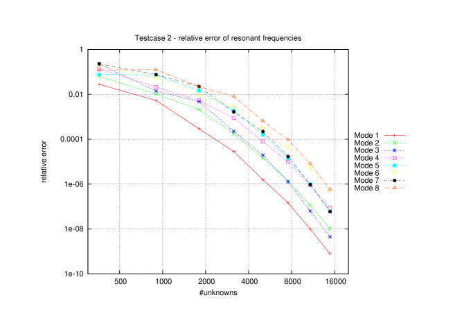
Figure 1: Convergence of the resonance frequencies after $p$-refinement

3 Computational aspects

As the spatial discretization conserves energy, we consider symplectic time integration methods which conserve the energy on a time-discrete level. The simplest one is the symplectic Euler method which discretizes the semi-discrete system (2) in the following way:

$$H^{n+1} = H^{n}+\Delta t\ M_{\mu}^{-1}C_{h}E^{n}$$

$$E^{n+1} = E^{n}-\Delta t\ M_{\varepsilon}^{-1}C_{h}^{T}H^{n+1}$$

with the stability condition

$$\Delta t\leq 2\left(\rho(M_{\mu}^{-\frac{1}{2}}C_{h}M_{e}^{-1}C_{h}^{T}M_{\mu}^{-\frac{1}{2}})\right)^{-1}$$

The matrix $M_{\mu}^{-\frac{1}{2}}C_{h}M_{e}^{-1}C_{h}^{T}M_{\mu}^{-\frac{1}{2}}$ is symmetric and the spectral radius $\rho$ can be estimated once by an iterative method like the power iteration.
When shifting the electric or the magnetic field by a half time-step we can reconstruct the well-known leap frog method. Nevertheless for our considerations it is less important which time integration scheme is used as long as it is explicit. The matrix multiplications with $C_{h}$ and $C_{h}^{T}$ (see Section 3.2) as well as with $M_{\mu}^{-1}$ and $M_{\varepsilon}^{-1}$ (see Section 3.3) decide about the computational efficiency of an implementation.

The advantage of discontinuous Galerkin methods becomes evident now. The mass matrices can be inverted in an element by element fashion and also the discrete $\operatorname{curl}$ operations only need information of (element-)local and adjacent degrees of freedom, which allows for straightforward parallelization. Element matrices such as mass matrices and the discrete $\operatorname{curl}$ operation can be stored once and applied at each time step. This is how far one comes just because of the formulation itself.

With appropriate choices for the local shape functions we can use advanced techniques to execute those operations with a lower complexity than local matrix-vector multiplications. Furthermore we don’t even have to store the element matrices, s.t. the techniques presented below are also much more memory-efficient.

The following ingredients are essential for the techniques proposed below, which enhance the implementation of the DG method:

1. Definition of an $L^{2}$-orthogonal basis of polynomial shape functions in tensor-product form on a reference element $\hat{T}$

2. Use of $\operatorname{curl}$-conforming (covariant) transformation for evaluations on the physical element $T$

3. Use of recurrences for the polynomial shape functions to evaluate gradients and $\operatorname{curl}$s

4. Use of tensor-product structure to evaluate traces

3.1 Local shape functions

For stability and fast computability we choose the $L_{2}$-orthogonal Dubiner basis [5, 9]. Here, the basis functions on the reference element are constructed in a tensor-product form of Jacobi polynomials $P_{i}^{(\alpha,\beta)}$ for each spatial component (note that the Legendre polynomials $P_{i}=P_{i}^{(0,0)}$ are just a special case). For example, on the reference triangle spanned by the points $(0,0)$, $(1,0)$ and $(0,1)$ the shape functions take the form

$$\varphi_{i,j}(x,y)=P_{i}\left(\textstyle\frac{2y}{1-x}-1\right)\cdot(1-x)^{i}\cdot P_{j}^{(2i+1,0)}(2x-1).$$ (6)

They are orthogonal on the reference triangle, and gradients can be evaluated by means of recurrence relations as demonstrated in Section 3.2.2. Due to the tensor-product form traces can be evaluated very fast, see Section 3.2.3.

3.2 Discrete $\operatorname{curl}$ operations

At each time step we have to evaluate terms like $(H,\operatorname{curl}e)_{T}$ on each element $T$ and $(\{\!\!\{H\}\!\!\}\times\nu,[\![e]\!])_{F}$ on each face $F$. Similar expressions have to be evaluated for the electric field $E$.

3.2.1 Covariant transformation

Let $\Phi:\hat{T}\rightarrow T$ be a diffeomorphic mapping from the reference element to some physical element $T$. Then the covariant transformation of a function $\hat{u}$ defined on the reference element $\hat{T}$ is

$$u:=(F^{-1})^{T}\hat{u}\circ\Phi^{-1}\qquad\mbox{ with }\qquad F=\nabla\Phi.$$

If we define the shape functions on the mapped elements as the covariant transformed shape functions on the reference element, then the tangential component on the mapped element depends only on the tangential component of the reference element. The transformation is called $\operatorname{curl}$-conforming as it ensures that for any function $\hat{u}\in H(\operatorname{curl},\hat{\Omega})$ the covariant transformed function $u$ lies in $H(\operatorname{curl},\Omega)$. Furthermore it preserves certain integrals, s.t. the following relations hold for the covariant transformations $H,e\in H(\operatorname{curl},T)$ of $\hat{H},\hat{e}\in H(\operatorname{curl},\hat{T})$:

$$\left|\int_{T}H\operatorname{curl}e\,\mathrm{d}x\right| = \left|\int_{\hat{T}}\hat{H}\operatorname{curl}\hat{e}\,\mathrm{d}x\right|,$$

$$\left|\int_{\partial T}(H\times\nu)e\,\mathrm{d}s\right| = \left|\int_{\partial\hat{T}}(\hat{H}\times\nu)\hat{e}\,\mathrm{d}s\right|.$$

This means that the integrals of these forms appearing in the formulation are independent of the geometry of the particular elements. The matrices can be computed once on the reference element. This trick was published in [4].

3.2.2 Evaluating gradients

For computing $\operatorname{curl}$s it is sufficient to evaluate gradients, since the $\operatorname{curl}$ is a certain linear combination of derivatives. We write the corresponding function $\hat{E}$ in modal representation, i.e.,

$$\hat{E}=\sum_{\alpha}a_{\alpha}\varphi_{\alpha},\ a_{\alpha}\in\mathbbm{R}^{3},$$

where the sum ranges over the finite collection of (scalar) shape functions defined on the reference element (in 2D the multi-index $\alpha$ is $(i,j)$ and in 3D $\alpha=(i,j,k)$). With the use of the covariant transformation, we just have to consider the integral on the reference element $\hat{T}$:

$$\int_{\hat{T}}\hat{h}\operatorname{curl}\hat{E}\,\mathrm{d}x.$$

The idea is now to take advantage of recurrence relations between derivatives of Jacobi polynomials and Jacobi polynomials itself. We aim for an operation which gives the coefficients $b_{\alpha}\in\mathbbm{R}^{3}$ representing the gradient

$$\nabla\hat{E}=\sum_{\alpha}b_{\alpha}\varphi_{\alpha}.$$

Then $L^{2}$-orthogonality can be used to evaluate the complete integral very fast.

For ease of presentation let’s consider the far more easy case of evaluating the derivative of a scalar one-dimensional function $v(x)=\sum_{i=0}^{n}v_{i}P_{i}(x),\ v_{i}\in\mathbbm{R}$ given in a modal basis of Legendre polynomials $P_{i}$, which fulfill the relation

$$P^{\prime}_{i+1}(x)=P^{\prime}_{i-1}(x)+(2i+1)P_{i}(x).$$ (7)

Then the problem is to find the modal representation of

$$v^{\prime}(x)=\sum_{i=0}^{n}v_{i}P_{i}^{\prime}(x)=\sum_{i=0}^{n-1}w_{i}P_{i}(x).$$

Let’s show the first step, i.e., how we get the highest order coefficient $w_{n-1}$:

$$v^{\prime}(x) = \sum_{i=0}^{n}v_{i}P_{i}^{\prime}(x)=\sum_{i=0}^{n-1}v_{i}P_{i}^{\prime}(x)+v_{n}P_{n}^{\prime}(x)$$

$$= \sum_{i=0}^{n-1}v_{i}P_{i}^{\prime}(x)+v_{n}P_{n-2}^{\prime}(x)+v_{n}(2n-1)P_{n-1}$$

$$= \sum_{i=0}^{n-1}\tilde{v}_{i}P_{i}^{\prime}(x)+w_{n-1}P_{n-1}(x)$$

where we used the recurrence relation (7) for $P_{n}^{\prime}(x)$ and thus get $w_{n-1}=v_{n}(2n-1)$. For the remaining polynomial $\sum_{i=0}^{n-1}\tilde{v}_{i}P_{i}^{\prime}(x)$ of degree $n-1$ we can apply the same procedure to get $w_{n-2}$. This can be continued until also $w_{0}$ and thereby the complete polynomial representation $\sum_{i=0}^{n-1}w_{i}P_{i}(x)$ of $v^{\prime}(x)$ is determined.

An efficient C++ implementation of this procedure was achieved by template meta-programming, where the compiler can generate optimized code for all elements up to an a priori chosen maximal polynomial order.

The same basically also works in three dimensions with Jacobi polynomials, but the relations are far more complicated, see Section 4, and need 3 nested loops.

The overall costs for the evaluation of the element $\operatorname{curl}$ integral scales linearly with the number of unknowns $N$ on one element which is much better than the matrix-vector multiplication which already has complexity $\mathcal{O}(N^{2})$.

3.2.3 Evaluating traces

The boundary integrals that have to be evaluated can make use of the tensor-product form to evaluate traces. Again we don’t want those traces to be evaluated pointwise but in a modal sense and recurrences for the Jacobi polynomials make the transformation from volume element shape functions to face shape functions with $\mathcal{O}(N)$ operations possible. The procedure therefore is similar to the evaluation of the gradient in the previous section.

3.3 Mass matrix operations

So far we dealt only with the discrete $\operatorname{curl}$ operations. So the only thing that is left to talk about is the application of the inverse mass matrices. Due to the covariant transformation we have

$$((M_{\varepsilon})_{\alpha,\beta})_{l,m} = \int_{T}\varepsilon\,(\varphi_{\alpha}e_{l}^{T})\,(\varphi_{\beta}e_{m})\,\mathrm{d}x$$ (8)

$$= \int_{\hat{T}}|\det(F)|\,\varepsilon\,(\hat{\varphi}_{\alpha}e_{l}^{T})F^{-1}(F^{-1})^{T}(\hat{\varphi}_{\beta}e_{m})\,\mathrm{d}x$$

with $\varphi_{\alpha}$ denoting the scalar-valued shape functions and $e_{n}$ the $n$-th unit vector. Note also the block structure of $M_{\varepsilon}$ that is indicated by the above notation. In some FEM applications, symbolic methods related to those described in Section 4, can be used to prove the sparseness of the corresponding system matrix, see [12].

3.3.1 Flat elements

Let’s assume the material parameters $\varepsilon$ and $\mu$ are piecewise constant and the elements are flat, i.e., $\nabla\Phi=F=const$ on each element. Then the integral (8) simplifies to

$$\int_{T}\varepsilon\,(\varphi_{\alpha}e_{l}^{T})\,(\varphi_{\beta}e_{m})\,\mathrm{d}x=|\det(F)|\,\varepsilon\,(F^{-1}(F^{-1})^{T})_{l,m}\int_{\hat{T}}\hat{\varphi}_{\alpha}\hat{\varphi}_{\beta}\,\mathrm{d}x$$

and as $\int_{\hat{T}}\hat{\varphi_{\alpha}}\hat{\varphi_{\beta}}\,\mathrm{d}x=\delta_{\alpha,\beta}$ the matrix is $(3\times 3)$-block-diagonal and the inversion is trivial. The computational effort is obviously of order $\mathcal{O}(N)$ where $N$ is the number of unknowns.

3.3.2 Curved elements

If we consider curved elements or non-constant material parameters $\varepsilon$ and $\mu$, the approach has to be modified as the mass matrix arising from (8) may be fully occupied. Let’s go a step back and consider a similar scalar problem with a non-constant coefficient $\varepsilon$:

Given: $$f(v)=\int_{T}fv\,\mathrm{d}x$$

Find: $$u,\text{ s.t. }\int_{T}\varepsilon uv\,\mathrm{d}x=\int_{T}fv\,\mathrm{d}x$$

We now transform back to the reference element $\hat{T}$ and get

$$\int_{T}\varepsilon uv\,\mathrm{d}x=\int_{\hat{T}}|\det(F)|\,\varepsilon uv\,\mathrm{d}x=\int_{\hat{T}}\hat{u}\tilde{v}\,\mathrm{d}x$$

where $\tilde{v}=|\det(F)|\,\varepsilon\hat{v}$. If we now approximate $\tilde{v}$ with the same basis we used for $v$ before, the mass matrix is diagonal again. Nevertheless the evaluation of the functional $f(v)$ has to be transformed as well:

$$\int_{T}fv\,\mathrm{d}x=\int_{T}\frac{1}{|\det(F)|\,\varepsilon}f\tilde{v}\,\mathrm{d}x=\int_{\hat{T}}\frac{1}{\varepsilon}f\tilde{v}\,\mathrm{d}x$$

To evaluate the last term we will use numerical integration. But as (in our application) $f$ is not given pointwise, but in a modal sense, we have to calculate a pointwise representation for the numerical integration of $\int_{T}fv\,\mathrm{d}x$ first:

Given: $$f(v)=\int_{T}fv\,\mathrm{d}x=\int_{\hat{T}}|\det(F)|\,f\hat{v}\,\mathrm{d}x$$

Find: $$f_{i},\text{ s.t. }\int_{T}fv\,\mathrm{d}x=\sum_{i}|\det(F)|(x_{i})f_{i}\omega_{i}v(x_{i})$$

Then we can divide (on each integration point) by $\varepsilon$ and with those new coefficients we can, by numerical integration, get a good approximation to $\int_{\hat{T}}\frac{1}{\varepsilon}f\tilde{v}\,\mathrm{d}x$. The “reverse numerical integration” and the numerical integration used here can be accelerated by the use of the sum factorization technique. Doing so the complexity of both “reverse numerical integration” and the numerical integration is $\mathcal{O}(p^{4})$, where $p$ is the polynomial degree. Note that the approximate inverse $\tilde{M}_{\varepsilon}^{-1}$ obtained by this method is still symmetric and positive definite.

3.4 Overall computational effort

In the previous sections we saw that the overall computational effort scales linearly with the degrees of freedom $N$ as long as the elements are flat and coefficients are piecewise constant. Even for curved elements (and variable coefficients) the computational effort is only of order $\mathcal{O}(N^{\frac{4}{3}})$. Furthermore no element matrices have to be stored. Only the geometric transformations and the local topology have to be kept in the memory.

3.5 Timings

Let’s also state some exemplary numbers that were achieved for this method and its implementation on an Intel Xeon CPU 5160 at $3.00$ GHz (64 bit) (single core) for a tetrahedral mesh with 2078 elements. The costs for one step of the symplectic Euler method per 6 scalar degrees of freedom are listed in Table 1.

order $p$	time $[\mu sec]$
1	0.61
2	0.58
3	0.71
4	0.79
5	1.16
6	1.24
7	1.32
8	1.53
9	1.66
10	1.74

order $p$	time $[\mu sec]$
1	4.89
2	2.54
3	1.93
4	1.79
5	2.06
6	2.17
7	2.33
8	2.67
9	2.88
10	3.04

Table 1: Timings for flat elements (left), using $\mathcal{O}(1)$ floating point operations per dof and curved elements (right) using $\mathcal{O}(p)$) floating point operations per dof.

4 Symbolic derivation of relations

In this section we want to describe the symbolic methods that were employed for finding the desired relations for the polynomial shape functions. These relations allow for efficient computation of the discrete curl operations and traces as described in Section 3.2. They have been computed by following the holonomic systems approach [13, 3, 10], which works for all functions that satisfy sufficiently many linear differential equations or recurrences or mixed ones; these relations have to have polynomial coefficients. A large class of functions (like rational or algebraic functions, exponentials, logarithms, and some of the trigonometric functions) as well as a multitude of special functions is covered by this framework. Part of it are algorithms for the “basic arithmetic” (that we will refer to as “closure properties”), i.e., given two implicit descriptions for functions $f$ and $g$, respectively, we can compute such descriptions for $f+g$, $fg$, and for functions obtained by certain substitutions into $f$ or $g$. All computations in this section have been performed in Mathematica using our package HolonomicFunctions (it is freely available from the website http://www.risc.uni-linz.ac.at/research/combinat/software/).

4.1 Introductory example

For demonstration purposes we show how to derive automatically the rewriting formula (7) for Legendre polynomials $P_{n}(x)$. It is well known that these orthogonal polynomials satisfy some linear relations, e.g., the second order differential equation

$$(x^{2}-1)P^{\prime\prime}_{n}(x)+2xP^{\prime}_{n}(x)-n(n+1)P_{n}(x)=0$$

or the three term recurrence

$$(n+2)P_{n+2}(x)-(2n+3)xP_{n+1}(x)+(n+1)P_{n}(x)=0.$$

We will represent such linear relations in the convenient operator notation, using the symbols $D_{\!x}$ for the partial derivative with respect to $x$, and $S_{\!n}$ for denoting the shift operator with respect to $n$. Then the two relations above are written as

$$(x^{2}-1)D_{\!x}^{2}+2xD_{\!x}+(-n^{2}-n)$$

and

$$(n+2)S_{\!n}^{2}+(-2nx-3x)S_{\!n}+(n+1),$$

respectively, and we identify operators and relations with each other. The operators can be regarded as elements of a (noncommutative) polynomial ring in $S_{\!n}$ and $D_{\!x}$ with coefficients being rational functions in $\mathbbm{Q}(n,x)$. We can obtain additional relations for $P_{n}(x)$ by combining the given relations linearly, or by shifting and differentiating them. In the operator setting these operations correspond to addition and multiplication (from the left) and we can refer to the set of all operators obtained in this way as the annihilating left ideal generated by the initially given operators. In the following we will represent annihilating ideals by means of their Gröbner bases; these are special sets of generators that allow for deciding the ideal membership problem (i.e., the question whether some relation is indeed valid for the function under consideration) and for obtaining unique representatives of the residue classes modulo the ideal (see [2]). All algorithms mentioned below will require Gröbner bases as input. A Gröbner basis of the annihilating ideal of the Legendre polynomials is given by

$$G=\big{\{}(n+1)S_{\!n}+(1-x^{2})D_{\!x}+(-nx-x),(x^{2}-1)D_{\!x}^{2}+2xD_{\!x}+(-n^{2}-n)\big{\}}.$$

Our main task will be to find elements with certain properties in an annihilating ideal; this can be done via an ansatz as we demonstrate now. The relation (7) that we are going to recover connects $P^{\prime}_{n+2}(x)$, $P^{\prime}_{n}(x)$, and $P_{n+1}(x)$, and its coefficients are free of $x$. These facts translate to an ansatz operator of the form

$$A=c_{1}(n)D_{\!x}S_{\!n}^{2}+c_{2}(n)D_{\!x}+c_{3}(n)S_{\!n}$$

where the coefficients $c_{i}$ are rational functions in $\mathbbm{Q}(n)$, and hence free of $x$ as required. We have to determine the $c_{i}$ such that the operator $A$ is an element of the left ideal $I$ generated by $G$, so that $A(P_{n}(x))=0$. For this purpose we use the Gröbner basis $G$ to compute the unique representation of the residue class of $A$ modulo $I$ (it is achieved by reduction). We have $A\in I$ if and only if the residue class is represented by the zero operator and hence we can equate all its coefficients to zero, obtaining the following two equations

$$c_{1}(2nx^{2}+3x^{2}-n-2)+c_{2}(n+1)+c_{3}(x^{2}-1) = 0,$$

$$c_{1}(n+1)(2n+3)x+c_{3}(n+1)x = 0.$$

Note that in these equations the variable $x$ occurs, since it is contained in the coefficients of $G$. We get a solution that is free of $x$ by performing a coefficient comparison with respect to this variable. This yields in the end the linear system

$$\begin{pmatrix}-n-2&n+1&-1\\ 2n+3&0&1\\ (n+1)(2n+3)&0&n+1\end{pmatrix}\begin{pmatrix}c_{1}\\ c_{2}\\ c_{3}\end{pmatrix}=0$$

whose solution is

$$c_{1}=-1,\quad c_{2}=1,\quad c_{3}=2n+3,$$

and this gives rise to the desired relation.

Now what do we do if we don’t know the exact shape of the ansatz as given here by $A$? Then we have to include all possible monomials $D_{\!x}^{i}S_{\!n}^{j}$ up to some total degree into our ansatz. Looping over the degree, we will finally find the relation, but the effort can be tremendous. Therefore, as a preprocessing step, we determine the shape of the ansatz by modular computations. This means plugging in concrete values for some of the variables and reducing all integers in the coefficients modulo some prime. These techniques have been described in detail in [10] and they are crucial for getting results in a reasonable time.

All these steps have been implemented in the package HolonomicFunctions and it computes the relation (7) immediately:

In[1]:=$\displaystyle<\!<\ \mathrm{HolonomicFunctions.m}$

HolonomicFunctions package by Christoph Koutschan, RISC-Linz, Version 1.3 (25.01.2010) $\longrightarrow$ Type ?HolonomicFunctions for help

In[2]:=$\displaystyle\mathrm{FindRelation}\big{[}\mathrm{Annihilator}[\mathrm{LegendreP}[n,x]],\>\mathrm{Eliminate}\to x\big{]}$

Out[2]=$\displaystyle\{S_{\!n}^{2}D_{\!x}+(-2n-3)S_{\!n}-D_{\!x}\}$

4.2 Relations for the shape functions

A core functionality of our package HolonomicFunctions [10] is to execute closure property algorithms (e.g., for addition, multiplication, and substitution) on functions represented by their annihilating ideals. We can now use these algorithms to obtain annihilating ideals for the shape functions $\varphi$, since their definition in terms of Jacobi and Legendre polynomials involves just the above mentioned operations.

4.2.1 The 2D case

We first consider triangular finite elements in two dimensions. For these, the shape functions are defined as in (6). Analogously to the one-dimensional example in Section 3.2.2 we want to express the partial derivatives (with respect to $x$ and $y$, respectively) in terms of the original shape functions. So the goal is to find relations (free of $x$ and $y$) that connect the partial derivatives with the original function. More concretely, we are looking for a relation that allows to express some linear combination of shifts of $\frac{\mathrm{d}}{\mathrm{d}x}\varphi_{i,j}(x,y)$ as a linear combination of shifts of $\varphi_{i,j}(x,y)$ (and similarly for $y$). This corresponds to an operator of the form

$$\sum_{(m,n)\in\mathbbm{N}^{2}}c_{1,m,n}(i,j)D_{\!x}S_{\!i}^{m}S_{\!j}^{n}+\sum_{(m,n)\in\mathbbm{N}^{2}}c_{0,m,n}(i,j)S_{\!i}^{m}S_{\!j}^{n}$$ (9)

where the yet unknown coefficients $c_{d,m,n}\in\mathbbm{Q}(i,j)$ do not depend on $x$ and $y$, and the sums have finite support.

Since we have to find such a relation in the annihilating ideal for $\varphi_{i,j}(x,y)$, it is natural to start by computing a Gröbner basis for this ideal. The package HolonomicFunctions provides a command Annihilator that analyzes a given mathematical expression and performs the necessary closure properties for obtaining its annihilating ideal. So in our example we can just type

In[3]:=$\displaystyle\mathrm{ann}=\mathrm{Annihilator}[(1-x)\mathbin{\raisebox{-2.5pt}{\hbox{\large$\hat{}$}}}i*\mathrm{LegendreP}[i,2y/(1-x)-1]*\hfil\break\hbox{}\qquad\qquad\qquad\mathrm{JacobiP}[j,2i+1,0,2x-1],\{\mathrm{S}[i],\,\mathrm{S}[j],\,\mathrm{Der}[x],\,\mathrm{Der}[y]\}];$

and after a second we have the result (which is already respectable in size, namely 340kB, corresponding to about 10 pages of output).

Having implemented noncommutative Gröbner bases, our first attempt was to use them for eliminating the variables $x$ and $y$. But it soon turned out that this attempt did not produce optimal results, and in addition the computations were very time-consuming. Therefore we came up with the ansatz described in Section 4.1. We use it now to compute the desired relations (both computations take less than a minute):

In[4]:=$\displaystyle\mathrm{FindRelation}[\mathrm{ann},\mathrm{Eliminate}\to\{x,y\},\mathrm{Pattern}\to\{\underline{\;\;},\underline{\;\;},0\mid 1,0\}]\hfil\break\hbox{}\qquad\mathop{\;/\!/\;}\mathrm{Factor}$

Out[4]=$\displaystyle\{(2i+j+5)(2i+2j+5)S_{\!i}S_{\!j}^{2}D_{\!x}+(j+3)(2i+2j+5)S_{\!j}^{3}D_{\!x}+\hfil\break\hbox{}\phantom{\{}2(2i+3)(i+j+3)S_{\!i}S_{\!j}D_{\!x}-2(2i+1)(i+j+3)S_{\!j}^{2}D_{\!x}-\hfil\break\hbox{}\phantom{\{}2(i+j+3)(2i+2j+5)(2i+2j+7)S_{\!i}S_{\!j}-(j+1)(2i+2j+7)S_{\!i}D_{\!x}-\hfil\break\hbox{}\phantom{\{}2(i+j+3)(2i+2j+5)(2i+2j+7)S_{\!j}^{2}-(2i+j+3)(2i+2j+7)S_{\!j}D_{\!x}\}$

In[5]:=$\displaystyle\mathrm{FindRelation}[\mathrm{ann},\mathrm{Eliminate}\to\{x,y\},\mathrm{Pattern}\to\{\underline{\;\;},\underline{\;\;},0,0\mid 1\}]\hfil\break\hbox{}\qquad\mathop{\;/\!/\;}\mathrm{Factor}$

Out[5]=$\displaystyle\{(2i+j+6)(2i+j+7)(2i+2j+7)S_{\!i}^{2}S_{\!j}^{2}D_{\!y}-(j+3)(j+4)(2i+2j+7)S_{\!j}^{4}D_{\!y}-\hfil\break\hbox{}\phantom{\{}4(j+2)(i+j+4)(2i+j+6)S_{\!i}^{2}S_{\!j}D_{\!y}+4(j+3)(i+j+4)(2i+j+5)S_{\!j}^{3}D_{\!y}+\hfil\break\hbox{}\phantom{\{}(j+1)(j+2)(2i+2j+9)S_{\!i}^{2}D_{\!y}-4(2i+3)(i+j+4)(2i+2j+7)(2i+2j+9)S_{\!i}S_{\!j}^{2}-\hfil\break\hbox{}\phantom{\{}(2i+j+4)(2i+j+5)(2i+2j+9)S_{\!j}^{2}D_{\!y}\}$

Here the option Pattern specifies the admissible exponents for the operators, e.g., in the first case we allow any exponent for the shift operators, whereas $D_{\!x}$ may occur with power at most $1$ only, and $D_{\!y}$ must not appear at all in the result.

4.2.2 The 3D case

When dealing with tetrahedra in three dimensions, the shape functions are denoted by $\varphi_{i,j,k}(x,y,z)$ and are defined by

$$(1-x-y)^{i}(1-x)^{j}P_{i}\!\left(\textstyle\frac{2z}{1-x-y}-1\right)P_{j}^{(2i+1,0)}\!\left(\textstyle\frac{2y}{1-x}-1\right)P_{k}^{(2i+2j+2,0)}(2x-1).$$

Again they have the nice property of being $L^{2}$-orthogonal on the reference tetrahedron

$$T=\{(x,y,z)\in\mathbbm{R}^{3}\mid x\geq 0\land y\geq 0\land z\geq 0\land x+y+z\leq 1\}.$$

Computing an annihilating ideal for $\varphi_{i,j,k}(x,y,z)$ is already much more involved than in the 2D case:

In[6]:=$\displaystyle\mathrm{phi}=(1-x-y)\mathbin{\raisebox{-2.5pt}{\hbox{\large$\hat{}$}}}i\,(1-x)\mathbin{\raisebox{-2.5pt}{\hbox{\large$\hat{}$}}}j\,\mathrm{LegendreP}[i,2z/(1-x-y)-1]\hfil\break\hbox{}\qquad\mathrm{JacobiP}[j,2i+1,0,2y/(1-x)-1]\,\mathrm{JacobiP}[k,2i+2j+2,0,2x-1];$

In[7]:=$\displaystyle\mathrm{Timing}[\mathrm{ann}=\mathrm{Annihilator}[\mathrm{phi},\>\{\mathrm{Der}[x],\,\mathrm{S}[i],\,\mathrm{S}[j],\,\mathrm{S}[k]\}];]$

Out[7]=$\displaystyle\{359.686,\mathrm{Null}\}$

The Gröbner basis for this annihilating ideal is about 117MB in size (corresponding to several thousand of printed pages). Note also that it is more efficient to consider only one derivation operator, and compute annihilating ideals for each of the cases $\frac{\mathrm{d}}{\mathrm{d}x}$, $\frac{\mathrm{d}}{\mathrm{d}y}$, and $\frac{\mathrm{d}}{\mathrm{d}z}$ separately (this applies to the 2D case, too).

In principle, the desired relations for the 3D case can be found in the same way as for two dimensions. As described in Section 4.1 we find by means of modular computations that the ansatz (for the case $\frac{\mathrm{d}}{\mathrm{d}x}$) contains the $16$ monomials

$$\begin{array}[]{l}S_{\!i}S_{\!j}S_{\!k}^{2}D_{\!x},S_{\!i}S_{\!k}^{3}D_{\!x},S_{\!j}^{2}S_{\!k}^{2}D_{\!x},S_{\!j}S_{\!k}^{3}D_{\!x},S_{\!i}S_{\!j}S_{\!k}D_{\!x},S_{\!i}S_{\!k}^{2}D_{\!x},S_{\!j}^{2}S_{\!k}D_{\!x},S_{\!j}S_{\!k}^{2}D_{\!x},\\ S_{\!i}S_{\!j}S_{\!k},S_{\!i}S_{\!j}D_{\!x},S_{\!i}S_{\!k}^{2},S_{\!i}S_{\!k}D_{\!x},S_{\!j}^{2}S_{\!k},S_{\!j}^{2}D_{\!x},S_{\!j}S_{\!k}^{2},S_{\!j}S_{\!k}D_{\!x}.\end{array}$$

However, in order to compute the corresponding coefficients, we did not succeed with the standard approach used in Section 4.2.1. Instead, we had to employ modular techniques again for many interpolation points, and then interpolate and reconstruct the solution.

5 Conclusion

We have presented an efficient implementation for solving the time-domain Maxwell’s equations with a finite element method that uses discontinuous Galerkin elements. Besides many other optimizations that speed up the whole simulation, the usage of certain recurrence relations for the shape functions allows for a fast evaluation of gradients and traces. These relations have been derived symbolically with computer algebra methods.

It is widely believed that the mathematical subjects “numerical analysis” and “symbolic computation” do not have much in common, or even that they are kind of orthogonal. Experts from both areas can barely communicate with each other unless they don’t talk about work. It was the great merit of the project SFB F013 “Numerical and Symbolic Scientific Computing” that had been established in 1998 at the Johannes Kepler University of Linz, Austria, to bring together these two communities to identify potential collaborations. We consider our results as a perfect example for such a fruitful cooperation.

Acknowledgement

We would like to thank Veronika Pillwein for making contact between the first- and the last-named author and for kindly supporting our work by interpreting between the languages of symbolics and numerics.

References

- [1] D. N. Arnold, F. Brezzi, B. Cockburn, D. Marini. Unified analysis of discontinuous Galerkin methods for elliptic problems. SIAM J. Numer. Anal. 39(5), 1749–1779 (2002)
- [2] B. Buchberger. Ein Algorithmus zum Auffinden der Basiselemente des Restklassenrings nach einem nulldimensionalen Polynomideal. Ph.D. thesis, University of Innsbruck, Austria (1965)
- [3] F. Chyzak. An extension of Zeilberger’s fast algorithm to general holonomic functions. Discrete Math. 217(1-3), 115–134 (2000)
- [4] G. Cohen, X. Ferries and S. Pernet. A spatial high-order hexahedral discontinuous Galerkin method to solve Maxwell’s equations in time domain. J. Comput. Phys. 217, 340–363 (2006)
- [5] M. Dubiner. Spectral methods on triangles and other domains. J. Sci. Comput. 6(4), 345–390 (1991)
- [6] J. S. Hesthaven and T. Warburton. Nodal Discontinuous Galerkin Methods—Algorithms, Analysis and Applications. Text in Applied Mathematics. Springer (2007)
- [7] J. S. Hesthaven and T. Warburton On the constants in hp-finite element trace inverse inequalities. Comput. Methods Appl. Mech. Eng. 192, 2765–2773 (2003)
- [8] P. Houston, I. Perugia and D. Schötzau. Mixed discontinuous Galerkin approximation of the Maxwell operator. SIAM J. Numer. Anal. 42(1), 434–459 (2004)
- [9] G. E. Karniadakis and S. J. Sherwin. Spectral/hp Element Methods for Computational Fluid Dynamics. Oxford Science Publications (2005)
- [10] C. Koutschan. Advanced Applications of the Holonomic Systems Approach. Ph.D. thesis, RISC, Johannes Kepler University, Linz, Austria (2009)
- [11] I. Perugia, D. Schötzau, and P. Monk. Stabilized interior penalty methods for the time-harmonic Maxwell equations. Comput. Methods Appl. Mech. Eng. 191, 4675–4697 (2002)
- [12] V. Pillwein. Computer Algebra Tools for Special Functions in High Order Finite Element Methods. Ph.D. thesis, Johannes Kepler University, Linz, Austria (2008)
- [13] D. Zeilberger. A holonomic systems approach to special functions identities. J. Comput. Appl. Math. 32(3), 321–368 (1990)