Distributed Self-Organization Of Swarms To Find Globally $\epsilon$-Optimal Routes To Locally Sensed Targets

Abstract

The problem of near-optimal distributed path planning to locally sensed targets is investigated in the context of large swarms. The proposed algorithm uses only information that can be locally queried, and rigorous theoretical results on convergence, robustness, scalability are established, and effect of system parameters such as the agent-level communication radius and agent velocities on global performance is analyzed. The fundamental philosophy of the proposed approach is to percolate local information across the swarm, enabling agents to indirectly access the global context. A gradient emerges, reflecting the performance of agents, computed in a distributed manner via local information exchange between neighboring agents. It is shown that to follow near-optimal routes to a target which can be only sensed locally, and whose location is not known a priori, the agents need to simply move towards its “best” neighbor, where the notion of “best” is obtained by computing the state-specific language measure of an underlying probabilistic finite state automata. The theoretical results are validated in high-fidelity simulation experiments, with excess of $10^{4}$ agents.

1 Introduction & Motivation

Path planning in a co-operative environment is a problem of great interest in multi-agent robotics. Recent developments in micro machining and MEMs have opened up the possibility of engineering extremely small and cheap robotic platforms in large numbers. Limited in size, on-board computational resources and power, such robots nevertheless can potentially exploit co-operation to accomplish complex tasks [DG89, Gage1992, Holl99, Unsal1994] including surveillance, reconnaissance, path finding and collaborative payload conveyance. However, coordinating such engineered swarms unveils new challenges not encountered in the operation of one or a few robots [Gage93, LB92, Payton01]. Coordination schemes requiring unique identities for each robot, explicit routing of point-to-point communication between robots, or centralized representations of the state of an entire swarm are no longer viable. Thus, any approach to effectively control swarms must be intrinsically scalable, and must only use information that is locally available. The immediate question for the control theorist is whether such algorithms are able to guarantee any level of global performance. This is precisely the problem that is investigated in this paper, with an affirmative answer; a distributed scalable control algorithm is proposed that allows very large swarms (simulation results obtained with $10^{4}$ agents) to self-organize and find near-global-optimal routes to locally known targets. The proposed algorithm uses only information that can be locally queried, and rigorous theoretical results on convergence, robustness, scalability are established, and effect of system parameters such as the agent-level communication radius and agent velocities on global performance is analyzed.

The fundamental philosophy of the proposed approach is to percolate local information across the swarm, enabling agents to indirectly access the global context. A gradient emerges, reflecting the performance of agents, computed in a distributed manner via local information exchange between neighboring agents. It is shown that to follow near-optimal routes to a target which can be only sensed locally, and whose location is not known a priori, the agents need to simply move towards its “best” neighbor, where the notion of “best” is obtained by computing the state-specific language measure [CR07] of an underlying probabilistic finite state automata [CR08].

Gradient based method in swarm control are not new [Payton01, STMRK09, NCD08, HW09]. Majority of reported work following this direction draw inspiration from swarming phenomena observed in nature, where self-organized exploration strategies emerge at the collective level as a result of simple rules followed by individual agents. To produce the global behavior, individuals interact by using simple and mostly local communication protocols. Social insects are a good biological example of organisms collectively exploring an unknown environment, and they have served as a source of direct inspiration for research on self-organized cooperative robotic exploration and path formation in groups of robots [Svennebring04, WL99]. The standard engineering approach to analyze desired global patterns and break them down into a set of simple rules governing individual agents is seldom applicable to large populations aspiring to accomplish complex tasks. Nevertheless some progress have been made in this direction [Couzin2005].

“We now know that such synchronized group behavior (of flocking birds) is mediated through sensory modalities such as vision, sound, pressure and odor detection. Individuals tend to maintain a personal space by avoiding those too close to themselves; group cohesion results from a longer-range attraction to others; and animals often align their direction of travel with that of nearby neighbors. These responses can account for many of the group structures we see in nature, including insect swarms and the dramatic vortex-like mills formed by some species of fish and bat. By adjusting their motion in response to that of near neighbors, individuals in groups both generate, and are influenced by, their social context — there is no centralized controller.” Collective Minds, D. Couzin [Couzin2007]

On the other hand, the Evolutionary Robotics (ER) methodology [Nolfi00] allows for an implementation of a top-down approach, where reinforcement learning via evolutionary optimization techniques allows assessment of the system’s overall performance, and sequentially improve control laws. While such heuristic techniques have been shown to yield robust and scalable systems, assuring global performance has remained an elusive challenge. The present paper aims to fill this gap by proposing a simple control approach with provable guarantees on global performance. The key difference with the reported gradient based techniques lies in the formal model that is developed, and the associated theoretical results that show that the algorithm achieves near-global optimality.

To the best of the author’s knowledge, such an approach has not been previously investigated, primarily due to the complexity spike encountered in deriving optimal solutions in a decentralized environment. Recent investigations [Bn00, BGIZ02] into the solution complexity of decentralized Markov decision processes have shown that the problem is exceptionally hard even for two agents; illustrating a fundamental divide between centralized and decentralized control of MDP. In contrast to the centralized approach, the decentralized case provably does not admit polynomial-time algorithms. Furthermore, assuming $\textrm{EXP}=\textrm{NEXP}$, the problems require super-exponential time to solve in the worst case. Furthermore, since distributed systems with access to only local information can be mapped to partially observable MDPs, it follows from [LGM01] that such problems are non-approximable, negating the possibility of obtaining optimal solutions to approximate representations.

Such negative results do not preclude the possibility of obtaining near-optimal solutions efficiently, when the set of models considered is a strictly smaller subset of general MDPs. This is precisely what we achieve in this paper; casting the path planning problem as a performance maximization problem for an underlying probabilistic finite state automata (PFSA). In spite of similar Markovian assumptions, the PFSA model is distinct from the general MDPS (See Section 2.1), and admits decentralized manipulation, such that the control policy, on convergence, is within an $\epsilon$ bound of the global optimal. Furthermore, one can freely choose the error bound $\epsilon$ (and make it as small as one wishes), with the caveat that the convergence time increases (with no finite upper bound) with decreasing $\epsilon$.

The present work is also distinct from Potential Field-based methodologies (PFM) widely studied in the centralized single-or-few robot scenarios [KGZ07, SHK08]. Early PFM implementations had substantial shortcomings [BK91-1] suffering from trap situations, instability in narrow passages $etc$. Some of these shortcomings have been addressed recently, leading to globally convergent potential planners [Volpe1990, Connolly1997, Vascak2007, KK93, S93, AKH08, WM03]. These approaches are computationally hard for single-or-few robots, and thus not applicable in the current context. Some variations of the latter approaches have attempted to reduce the complexity by combining search algorithms and potential fields [Shar1993, Barraquand1992, Barraquand1991], virtual obstacle methods method [Park2003, Li2000], sub-goal methods [Bell2004, Weir2006], wall-following methods [Borenstein1989, Yun1997, Park2003, Mabrouk2008w] etc. Nevertheless, since heuristic strategies only based on local environment information are usually applied, many of these methods cannot guarantee convergence in general.

The rest of the paper is organized in six sections. Section 2 briefly summarizes the theory of quantitative measures of probabilistic regular languages, and the pertinent approaches to centralized performance maximization of PFSA. Section 3 develops the PFSA model for a swarm, and Section 4 presents the theoretical development for decentralized PFSA optimization, thus solving the problem of computing $\epsilon$-optimal routes in a static or frozen swarm. Section LABEL:secMob extends the results to a dynamic swarm, where route optimization and positional updates are carried out simultaneously. Section LABEL:sec6 validates the theoretical development with high fidelity simulation results. The paper concludes in Section LABEL:sec7 with recommendations for future work.

2 Background: Language Measure Theory

This section summarizes the concept of signed real measure of probabilistic regular languages, and its application in performance optimization of probabilistic finite state automata (PFSA) [CR07]. A string over an alphabet ($i.e.$ a non-empty finite set) $\Sigma$ is a finite-length sequence of symbols from $\Sigma$ [HMU01]. The Kleene closure of $\Sigma$, denoted by $\Sigma^{*}$, is the set of all finite-length strings of symbols including the null string $\epsilon$. $xy$ is the concatenation of strings $x$ and $y$, and the null string $\epsilon$ is the identity element of the concatenative monoid.

Definition 1 (PFSA).

A PFSA $G$ over an alphabet $\Sigma$ is a sextuple $(Q,\Sigma,\delta,\widetilde{\Pi},\chi,$ $\mathscr{C})$, where $Q$ is a set of states, $\delta:Q\times\Sigma^{\star}\rightarrow Q$ is the (possibly partial) transition map; $\widetilde{\Pi}:Q\times\Sigma\rightarrow[0,1]$ is an output mapping or the probability morph function that specifies the state-specific symbol generation probabilities, satisfying $\forall q_{i}\in Q,\sigma\in\Sigma,\widetilde{\Pi}(q_{i},\sigma)\geqq 0$, and $\sum_{\sigma\in\Sigma}\widetilde{\Pi}(q_{i},\sigma)=1$, the state characteristic function $\chi:Q\rightarrow[-1,1]$ assigns a signed real weight to each state reflecting the immediate pay-off from visiting that state, and $\mathscr{C}$ is the set of controllable transitions that can be disabled (See Definition 2) by an imposed control policy.

Definition 2 (Control Philosophy).

If $\delta(q_{i},\sigma)=q_{k}$, then the disabling of $\sigma$ at $q_{i}$ prevents the state transition from $q_{i}$ to $q_{k}$. Thus, disabling a transition $\sigma$ at a state $q$ replaces the original transition with a self-loop with identical occurrence probability, $i.e.$ we now have $\delta(q_{i},\sigma)=q_{i}$. Transitions that can be so disabled are controllable, and belong to the set $\mathscr{C}$.

Definition 3.

The language $L(q_{i})$ generated by a PFSA $G$ initialized at the state $q_{i}\in Q$ is defined as: $L(q_{i})=\{s\in\Sigma^{*}\ |\ \delta(q_{i},s)\in Q\}$ Similarly, for every $q_{j}\in Q$, $L(q_{i},q_{j})$ denotes the set of all strings that, starting from the state $q_{i}$, terminate at the state $q_{j}$, i.e., $L(q_{i},q_{j})=\{s\in\Sigma^{*}\ |\ \delta(q_{i},s)=q_{j}\in Q\}$

Definition 4 (State Transition Matrix).

The state transition probability matrix $\Pi\in[0,1]^{\textrm{{Card}}(Q)\times\textrm{{Card}}(Q)}$, for a given PFSA is defined as: $\forall q_{i},q_{j}\in Q,\Pi_{ij}=\sum_{\sigma\in\Sigma\ \mathrm{s.t.}\ \delta(q_{i},\sigma)=q_{j}}\widetilde{\Pi}(\sigma,q_{i})$ Note that $\Pi$ is a square non-negative stochastic matrix [BR97], where $\Pi_{ij}$ is the probability of transitioning from $q_{i}$ to $q_{j}$.

Notation 1.

We use matrix notations interchangeably for the morph function $\widetilde{\Pi}$. In particular, $\widetilde{\Pi}_{ij}=\widetilde{\Pi}(q_{i},\sigma_{j})$ with $q_{i}\in Q,\sigma_{j}\in\Sigma$. Note that $\widetilde{\Pi}\in[0,1]^{\textrm{{Card}}(Q)\times\textrm{{Card}}(\Sigma)}$ is not necessarily square, but each row sums up to unity.

A signed real measure [R88] $\nu^{i}:{2^{L(q_{i})}}\rightarrow\mathbb{R}\equiv(-\infty,+\infty)$ is constructed on the $\sigma$-algebra $2^{L(q_{i})}$ [CR07], implying that every singleton string set $\{s\in L(q_{i})\}$ is a measurable set.

Definition 5 (Language Measure).

Let $\omega\in L(q_{i},q_{j})\subseteq 2^{L(q_{i})}$. The signed real measure $\nu^{i}_{\theta}$ of every singleton string set $\{\omega\}$ is defined as: $\nu^{i}_{\theta}(\{\omega\})\triangleq\theta(1-\theta)^{|\omega|}\widetilde{\Pi}(q_{i},\omega)\chi(q_{j})$. For every choice of the parameter $\theta\in(0,1)$, the signed real measure of a sublanguage $L(q_{i},q_{j})\subseteq L(q_{i})$ is defined as: $\nu^{i}_{\theta}(L(q_{i},q_{j}))\triangleq\sum_{\omega\in L(q_{i},q_{j})}\theta(1-\theta)^{|\omega|}\widetilde{\Pi}(q_{i},\omega)\chi_{j}$. The measure of $L(q_{i})$, is defined as $\nu^{i}_{\theta}(L(q_{i}))\triangleq\sum_{q_{j}\in Q}\nu^{i}_{\theta}(L_{i,j})$.

Notation 2.

For a given PFSA, we interpret the set of measures $\nu^{i}_{\theta}(L(q_{i}))$ as a real-valued vector of length $\textrm{{Card}}(Q)$ and denote $\nu^{i}_{\theta}(L(q_{i}))$ as $\nu_{\theta}|_{i}$.

The language measure can be expressed vectorially as (where the inverse exists for $\theta\in(0,1]$ [CR07]):

$$\nu_{\theta}=\theta\big{[}\mathbb{I}-(1-\theta)\Pi\big{]}^{-1}\chi$$ (1)

In the limit of $\theta\rightarrow 0^{+}$, the language measure of singleton strings can be interpreted to be product of the conditional generation probability of the string, and the characteristic weight on the terminating state. Hence, smaller the characteristic, or smaller the probability of generating the string, smaller is its measure. Thus, if the characteristic values are chosen to represent the control specification, with more positive weights given to more desirable states, then the measure represents how good the particular string is with respect to the given specification, and the given model. The limiting language measure $\nu_{0}|_{i}=\lim_{\theta\rightarrow 0^{+}}\theta\big{[}\mathbb{I}-(1-\theta)\Pi\big{]}^{-1}\chi\big{|}_{i}$ sums up the limiting measures of each string starting from $q_{i}$, and thus captures how good $q_{i}$ is, based on not only its own characteristic, but on how good are the strings generated in future from $q_{i}$. It is thus a quantification of the impact of $q_{i}$, in a probabilistic sense, on future dynamical evolution [CR07].

Definition 6 (Supervisor).

A supervisor is a control policy disabling a specific subset of the set $\mathscr{C}$ of controllable transitions. Hence there is a bijection between the set of all possible supervision policies and the power set $2^{\mathscr{C}}$.

Language measure allows quantitative comparison of different supervision policies.

Definition 7 (Optimal Supervision Problem).

Given $G=(Q,\Sigma,\delta,\widetilde{\Pi},\chi,\mathscr{C})$, compute a supervisor disabling $\mathscr{D}^{\star}\subseteq\mathscr{C}$, s.t. $\nu^{\star}_{0}\geqq_{\textbf{{(Elementwise)}}}\nu^{{\dagger}}_{0}\ \ \forall\mathscr{D}^{{\dagger}}\subseteq\mathscr{C}$ where $\nu^{\star}_{0}$, $\nu^{{\dagger}}_{0}$ are the limiting measure vectors of supervised plants $G^{\star}$, $G^{{\dagger}}$ under $\mathscr{D}^{\star}$, $\mathscr{D}^{\dagger}$ respectively.

The solution to the optimal supervision problem is obtained in [CR07] by designing an optimal policy using $\nu_{\theta}$ with $\theta\in(0,1)$. To ensure that the computed optimal policy coincides with the one for $\theta\rightarrow 0^{+}$, the authors choose a small non-zero value for $\theta$ in each iteration step of the design algorithm. To address numerical issues, algorithms reported in [CR07] computes how small a $\theta$ is actually sufficient to ensure that the optimal solution computed with this value of $\theta$ coincides with the optimal policies for any smaller value, $i.e.$, computes the critical lower bound $\theta_{\star}$. (This is closely related to the notion of Blackwell optimality; See Section 2.1) Moreover the solution obtained is stationary, efficiently computable, and can be shown to be the unique maximally permissive policy among ones with maximal performance. Language-measure-theoretic optimization is not a search (and has several key advantages over Dynamic Programming based approaches. See Section 2.1 for details); it is an iterative sequence of combinatorial manipulations, that monotonically improves the measures, leading to element-wise maximization of $\nu_{\theta}$ (See [CR07]). It is shown in [CR07] that $\lim_{\theta\rightarrow 0^{+}}\theta\big{[}\mathbb{I}-(1-\theta)\Pi\big{]}^{-1}\chi=\mathscr{P}\chi$, where the $i^{th}$ row of $\mathscr{P}$ (denoted as $\wp^{i}$) is the stationary probability vector for the PFSA initialized at state $q_{i}$. In other words, $\mathscr{P}$ is the Cesaro limit of the stochastic matrix $\Pi$, satisfying $\mathscr{P}=\lim_{k\rightarrow\infty}\frac{1}{k}\sum_{j=0}^{k-1}\Pi^{j}$ [BR97].

Proposition 1 (See [CR07]).

Since the optimization maximizes the language measure element-wise for $\theta\rightarrow 0^{+}$, it follows that for the optimally supervised plant, the standard inner product $\langle\wp^{i},\chi\rangle$ is maximized, irrespective of the starting state $q_{i}\in Q$.

Notation 3.

The optimal $\theta$-dependent measure for a PFSA is denoted as $\nu^{\star}_{\theta}$ and the limiting measure as $\nu^{\star}$.

input : $\mathbf{P},\ \boldsymbol{\chi},\ \mathscr{C}$

output : Optimal set of disabled transitions $\mathscr{D}^{\star}$

begin  Set $\mathscr{D}^{[0]}=\emptyset$ ;  /* Initial disabling set */

Set $\widetilde{\Pi}^{[0]}=\widetilde{\Pi}$ ;  /* Initial event prob. matrix */

Set $\theta^{[0]}_{\star}=0.99$, Set $k\ =\ 1$ , Set $\texttt{Terminate}=$ false ;

while (Terminate == false) do  Compute $\theta_{\star}^{[k]}$;  /* Algorithm 2 */

Set $\widetilde{\Pi}^{[k]}=\frac{1-\theta_{\star}^{[k]}}{1-\theta_{\star}^{[k-1]}}\widetilde{\Pi}^{[k-1]}$;

Compute $\boldsymbol{\nu}^{[k]}$ ;

for $j=1$ to $n$ do  for $i=1$ to $n$ do  Disable all controllable $q_{i}\xrightarrow[]{\sigma}q_{j}$ s.t. $\boldsymbol{\nu}^{[k]}_{j}<\boldsymbol{\nu}^{[k]}_{i}$ ;

Enable all controllable $q_{i}\xrightarrow[]{\sigma}q_{j}$ s.t. $\boldsymbol{\nu}^{[k]}_{j}\geqq\boldsymbol{\nu}^{[k]}_{i}$ ;

    Collect all disabled transitions in $\mathscr{D}^{[k]}$;

if $\mathscr{D}^{[k]}==\mathscr{D}^{[k-1]}$ then  $\texttt{Terminate}=$ true ;

else  $k\ =\ k\ +\ 1$ ;

    $\mathscr{D}^{\star}\ =\ \mathscr{D}^{[k]}$ ;  /* Optimal disabling set */

end

Algorithm 1 Computation of Optimal Supervisor

input : $\mathbf{P},\ \boldsymbol{\chi}$

output : $\theta_{\star}$

begin  Set $\theta_{\star}=1$, Set $\theta_{curr}=0$;

Compute $\mathscr{P}$ , $M_{0}$ , $M_{1}$, $M_{2}$;

for $j=1$ to $n$ do  for $i=1$ to $n$ do  if $\left(\mathscr{P}\boldsymbol{\chi}\right)_{i}-\left(\mathscr{P}\boldsymbol{\chi}\right)_{j}\neq 0$ then  $\theta_{curr}=\frac{1}{8M_{2}}\big{|}\left(\mathscr{P}\boldsymbol{\chi}\right)_{i}-\left(\mathscr{P}\boldsymbol{\chi}\right)_{j}\big{|}$ else  for $r=0$ to $n$ do  if $\left(M_{0}\boldsymbol{\chi}\right)_{i}\neq\left(M_{0}\boldsymbol{\chi}\right)_{j}$ then  Break;

else  if $\left(M_{0}M_{1}^{r}\boldsymbol{\chi}\right)_{i}\neq\left(M_{0}M_{1}^{r}\boldsymbol{\chi}\right)_{j}$ then  Break;

      if $r==0$ then  $\theta_{curr}=\frac{|\left\{(M_{0}-\mathscr{P})\boldsymbol{\chi}\right\}_{i}-\left\{(M_{0}-\mathscr{P})\boldsymbol{\chi}\right\}_{j}|}{8M_{2}}$;

else  if $r>0$ AND $r\leq n$ then  $\theta_{curr}=\frac{|\left(M_{0}M_{1}\boldsymbol{\chi}\right)_{i}-\left(M_{0}M_{1}\boldsymbol{\chi}\right)_{j}|}{2^{r+3}M_{2}}$ ;

else  $\theta_{curr}=1$ ;

    $\theta_{\star}$ = $\mathrm{min}(\theta_{\star},\theta_{curr})$ ;

    end

Algorithm 2 Computation of the Critical Lower Bound $\theta_{\star}$

9

9

9

9

9

9

9

9

9

9

9

9

9

9

9

9

9

9

For completeness, the key algorithms are included as Algorithms 1 and 2.

2.1 Relation Of The Centralized Approach To Dynamic Programming

In spite of underlying Markovian assumptions, the PFSA model is distinct from the standard formalism of (finite state) Controlled Markov Decision Processes (CMDP) [FS02, Bertsekas1978, Bertsekas1987]. In the latter, control actions are not probabilistic; the associated control function maps states to unique actions in a deterministic manner, and the control problem is to decide which of the available control actions should be executed in each state. On the other hand, in the PFSA formalism, control is exerted by selectively disabling controllable probabilistic state transitions, and is thus a probabilistic generalization of supervisory control theory [RW87]. Note that while in the MDP framework, one specifies which control action to take at a given state, in the PFSA formalism one specifies which of the available control actions are not allowed at the current state, and that any of the remaining can be executed in accordance to their generation probabilities. Denoting the set of controllable transitions at state $q_{k}$ as $\Sigma_{C}$, and $\phi:Q\rightarrow\Sigma_{C}$ as the control policy mapping the current state $q_{k}\in Q$ to the controllable move $\phi(q_{k})\in\Sigma_{C}$ (and assuming that the control action is to dictate the agent to execute a specific controllable move and is not supervisory in nature), one can formulate an analogous optimization problem that admits solution within the DP framework. The transition probabilities for a stationary policy $\phi$ is given by:

$$\forall q_{i},q_{j}\in Q,\sigma_{r}\in\Sigma_{C},Prob(q_{j}\big{|}q_{i},\phi(q_{i})=\sigma_{r})=\sum_{\mathclap{\sigma\textrm{ s.t. }\left(\sigma\in\Sigma\setminus\Sigma_{C}\cup\{\sigma_{r}\}\right)\bigwedge\left(\delta(q_{i},\sigma)=q_{j}\right)}}\tilde{\pi}(q_{i},\sigma)$$ (2)

Immediate rewards, in DP terminology, can be related to the state characteristic $\chi$:

$$g(q_{i},\phi(q_{i}))=\chi(q_{i})$$ (3)

We note that the problem at hand must be solved over an infinite horizon, since the total number of transitions ($i.e.$ the path length) is not bounded. Identifying $(1-\theta)$ as the discount factor, the cost-to-go (to be maximized) for the infinite horizon discounted cost (DC) problem is given by:

$$J(q_{0},\phi)=\lim_{N\rightarrow\infty}\mathbf{E}\left(\sum_{i=0}^{N}(1-\theta)^{i}g\big{(}q_{i},\phi(q_{i})\big{)}\right)$$ (4)

and for the infinite horizon Average Cost per stage (AC):

$$J(q_{0})=\lim_{N\rightarrow\infty}\frac{1}{N}\mathbf{E}\left(\sum_{i=0}^{N}g\big{(}q_{i},\phi(q_{i})\big{)}\right)$$ (5)

AC is more appropriate, since there is no reason to ”discount” events in future. In the PFSA formalism, we solve the analogous discounted problem at sufficiently small $\theta$, and guarantee that the solution is simultaneously average cost optimal, primarily due to the following identity [CR07]:

$$\lim_{\theta\rightarrow 0^{+}}\theta\sum_{k=0}^{\infty}(1-\theta)^{k}\Pi^{k}\chi=\lim_{N\rightarrow\infty}\frac{1}{N}\sum_{j=0}^{N-1}\Pi^{j}\chi=\mathscr{P}\chi$$ (6)

where $\mathscr{P}$ is the Cesaro limit of the stochastic matrix $\Pi$. Thus, the proposed technique can solve the problem by maximizing

$$\nu_{\theta}=\lim_{\theta\rightarrow 0^{+}}\theta\sum_{k=0}^{\infty}(1-\theta)^{k}\Pi^{k}\chi=\lim_{\theta\rightarrow 0^{+}}\theta\big{[}\mathbb{I}-(1-\theta)\Pi\big{]}^{-1}\chi$$ (7)

$i.e.$, the language measure, and achieve maximization of $\mathscr{P}\chi$ (guaranteeing the probability of reaching the goal is maximized, while simultaneously minimizing collision probability). In any case, the formulated DP problem can be solved using standard solution methodologies such as Value Iteration (VI) or Policy Iteration (PI) [Put90, GS75]. We note that for VI, we need to search for the control action that maximizes the value update over all possible control actions, in each iteration. On the other hand, PI involves two steps in each iteration: (1) policy evaluation, which is very similar to the measure computation step in each iteration for the language-measure-theoretic technique and (2) policy improvement, which involves searching for a improved action over possible control actions for each state (which involves at least one product between a $\textrm{{Card}}(Q)\times\textrm{{Card}}(Q)$ matrix of transition probabilities and the current cost vector of length $\textrm{{Card}}(Q)$ per state). The disabling/enabling of controllable transitions is significantly simpler compared to the search steps that both VI and PI require, and the improvement in complexity (for PI which is closer to the proposed algorithm in the centralized case, since the latter proceeds via computing a sequence of monotonically improving policies) is by at least an asymptotic factor of $O(\textrm{{Card}}(Q)^{2})$ per iteration (for dense matrices, and $O(\textrm{{Card}}(Q))$ per iteration in the sparse case), which is significant for large problems.

Remark 1.

The number of iterations is not expected to be comparable for the PFSA framework, VI and PI techniques; simulations indicate the measure-theoretic approach converges faster, and detailed investigations in this direction is a topic of future work.

Another key advantage of the PFSA-based solution methodology is guaranteed Blackwell optimality [ABEFG93, FS02]. It is well recognized that the average cost criterion is underselective, namely the finite time behavior is completely ignored. The condition of Blackwell optimality attempts to correct this by demanding the computed controller be optimal for a continuous range of discount factors in the interval $(d_{0},1)$, $i.e.$ for $\theta\in(0,1-d_{0})$, where $0<d_{0}<1$. Since the PFSA-based approach maximizes the language measure for some $\theta=\theta_{min}$, such that the optimal policy is guaranteed to be identical for all values of $\theta$ in the range $[\theta_{min},0]$, the solution satisfies the Blackwell condition. It is possible to obtain such Blackwell optimal policies within the DP framework as well, but the approach(es) are significantly more involved (See [FS02], Chapter 8). The ability to adapt $\theta$ at each iteration (See Algorithm 2) leads to a novel adaptive discounting scheme in the technique proposed, which solves the infinite horizon problem efficiently while using a non-zero $\theta\geqq\theta_{min}$ at all iteration steps.

3 The Swarm Model

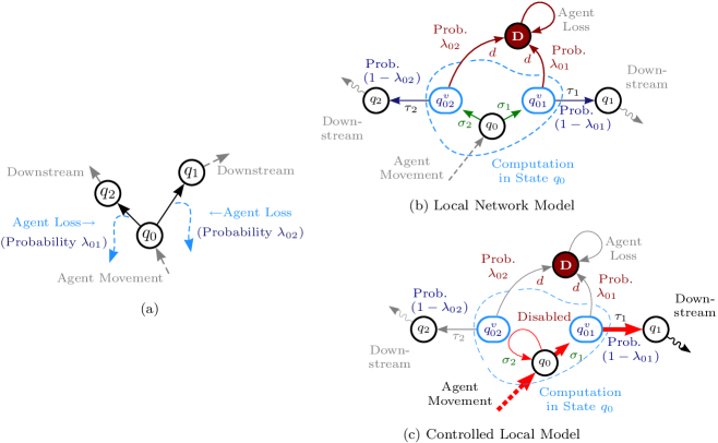
Fig. 1: Agent-centric local decision-making with non-zero failure probability

We consider ad-hoc mobile network of communicating agents endowed with limited computational resources. For simplicity of exposition, we develop the theoretical results under the assumption of a single target, or goal. This is not a serious restriction and can be easily relaxed. The location and identity of the target is not known a priori to the individual agents, only ones which are within the communication radius of the target can sense its presence. The communication radii are assumed to be constant throughout. Inter-agent communication links are assumed to be perfect, which again can be generalized easily, within our framework. We assume agents can efficiently gather the following information:

1. (Set of Neighboring agents:) Number and unique id. of agents to which it can successfully send data via a 1-hop direct line-of-sight link. The communication radius $R_{c}$ is assumed to be identical for each agent. The set of neighbors for each agent varies with time as the swarm evolves.

2. (Local Navigation Properties:) Navigation is assumed to occur by moving towards a chosen neighbor with constant velocity, the magnitude of which is assumed to be identical for each agent. In general, there a non-zero probability of agent failure in the course of execution this maneuver, which is assumed to be either known or learnable by the agents. However the explicit learning of these local costs is not addressed in this paper.

The local network model, along with the decision-making philosophy, is illustrated in Figure 1. We will talk about a frozen swarm, which denotes a particular spatial configuration of the agents assumed to be fixed in time. Unless explicitly mentioned, the agents are assumed to be updating their positions in continuous time (moving with constant velocity), while changing their headings in discrete time as dictated via on-board decision-making based on locally available information, with the objective of reaching the target with minimum end-to-end probability of agent failure. We further assume that the failure probabilities mentioned above are functions of the agent locations, and possibly vary in a smooth non-increasing manner with increasing inter-agent distances. However no time-dependence is assumed, $i.e.$ the failure probabilities remain constant for a frozen swarm, and change (due to the positional updates) for a mobile one. The agent velocities are assumed to be significantly slower compared to the time required for the convergence of the optimization algorithm for each frozen configuration. The implications of the last assumption will be discussed in the sequel. First we formalize a failure-prone ad-hoc network of frozen communicating agents as a probabilistic finite state automata.

Definition 8 (Neighbor Map For A Frozen Swarm).

If $Q$ is the set of all agents in the network, then the neighbor map $\mathcal{N}:Q\rightarrow 2^{Q}$ specifies, for each agent $q_{i}\in Q$, the set of agents $\mathcal{N}(q_{i})\subset Q$ (excluding $q_{i}$) to which $q_{i}$ can communicate via a single hop direct link.

Definition 9 (Failure Probability).

The failure probability $\lambda_{ij}\in[0,1]$ is defined to be the probability of unrecoverable loss of agent $q_{i}$ in the course of moving towards agent $q_{j}$.

Thus, $\lambda_{ij}$ reflects local or immediate navigation costs, and estimated risks and therefore varies with the positional coordinates of the agents $q_{i}$ and $q_{j}$. These quantities are not constrained to be symmetric in general, $i.e.$, $\lambda_{ij}\neq\lambda_{ji}$. We assume the agent-based estimation of these ratios to converge fast enough, in the scenario where such parameters are learned on-line. Since we are more concerned with decision optimization in this paper, we ignore the parameter estimation problem of learning the failure probabilities, which is at least intuitively justified by the existence of separated policies in large classes of similar problems.

We visualize the local network around a agent $q_{0}$ in a manner illustrated in Figure 1(a) (shown for two neighbors $q_{1}$ and $q_{2}$). In particular, agent $q_{0}$ attempting to move towards the current position of $q_{1}$ experiences a failure probability $\lambda_{01}$, while the moving towards $q_{2}$ has a failure probability $\lambda_{02}$. To correctly represent this information, we require the notion of virtual states ($q^{v}_{01},q^{v}_{02}$ in Figure 1(b)).

Remark 2 (Necessity Of Virtual States).

The virtual states are required to model the physical situation within the PFSA framework, in which transitions do not emerge from other transitions. As illustrated in Figure 1(a), the failure events do actually occur in the course of the attempted maneuver; hence necessitating the notion of the virtual states.

Definition 10 (Virtual State).

Given a agent $q_{i}$, and a neighbor $q_{j}\in\mathcal{N}(q_{i})$ with a specified failure probability $\lambda_{ij}$, any attempted move towards $q_{j}$ is assumed to be first routed to a virtual state $q^{v}_{ij}$, upon which there is either an automatic ($i.e.$ uncontrollable) forwarding to $q_{j}$ with probability $1-\lambda_{ij}$, or a failure with probability $\lambda_{ij}$. The set of all virtual states in a network of $Q$ agents is denoted by $Q^{v}$ in the sequel.

Hence, the total number of virtual states is given by:

$$\textrm{{Card}}(Q^{v})=\sum_{i:q_{i}\in Q}\mathcal{N}(q_{i})$$ (8)

And the cardinality of the set of virtual states satisfies:

$$0\leqq\textrm{{Card}}(Q^{v})\leqq\textrm{{Card}}(Q)^{2}-\textrm{{Card}}(Q)$$ (9)

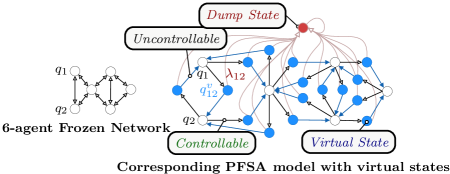
Fig. 2: 6-agent network & 23 state PFSA (16 virtual states, 6 agents, 1 dump state)

We assume that there is a static agent at the target or the goal, which we denote as $q_{\textrm{{Tgt}}}$. The local communication with this agent-at-target can be visualized as the process of sensing the target by the mobile agents. We are ready to model an ad-hoc communicating network of frozen agents as a PFSA, whose states correspond to either agents, the virtual states, or the state reflecting agent failures.

Definition 11 (PFSA Model of Frozen Network).

For a given set of agents $Q$, the function $\mathcal{N}:Q\rightarrow 2^{Q}$, the link specific failure probabilities $\lambda_{ij}$ for any agent $q_{i}$ and a neighbor $q_{j}\in\mathcal{N}(q_{i})$, and a specified target $q_{\textrm{{Tgt}}}\in Q$, the PFSA $\mathds{G}_{\textrm{{N}}}=(Q^{N},\Sigma,\delta,\widetilde{\Pi},\chi,\mathscr{C})$ is defined to be a model of the network, where (denoting $\textrm{{Card}}(\mathcal{N}(q_{i}))=m$):

$$\circ Q^{N}=Q\bigcup Q^{v}\bigcup\big{\{}q_{D}\big{\}}$$ States: (10a)

where $$Q^{v} q_{D}$$ is the set of virtual states, and is a dump state which models loss of agent due to failure.

$$\circ \Sigma=\bigcup_{i:q_{i}\in Q}\left(\bigcup_{j:q_{j}\in\mathcal{N}(q_{i})}\sigma_{ij}\right)\bigcup\big{\{}\sigma_{D}\big{\}}$$ Alphabet: (10b)

where $$\sigma_{ij} \sigma_{D}$$ denotes navigation (attempted or actual) denotes agent failure.

$$\circ \delta(q,\sigma)=\left\{\begin{array}[]{cl}q^{v}_{ij}&\textrm{if }q=q_{i},\sigma=\sigma_{ij}\\ q_{j}&\textrm{if }q=q^{v}_{ij},\sigma=\sigma_{ij}\\ q_{D}&\textrm{if }q=q^{v}_{ij},\sigma=\sigma_{D}\\ q_{D}&\textrm{if }q=q_{D},\sigma=\sigma_{D}\\ -&\textrm{undefined otherwise}\end{array}\right.$$ Transition Map: (10i)

$$\circ \widetilde{\Pi}(q,\sigma)=\left\{\begin{array}[]{cl}\frac{1}{m}&\textrm{if }q=q_{i},\sigma=\sigma_{ij}\\ 1-\lambda_{ij}&\textrm{if }q=q^{v}_{ij},\sigma=\sigma_{ij}\\ \lambda_{ij}&\textrm{if }q=q^{v}_{ij},\sigma=\sigma_{D}\\ 1&\textrm{if }q=q_{D},\sigma=\sigma_{D}\\ 0&\textrm{otherwise}\end{array}\right.$$ Probability Morph Matrix: (10p)

$$\circ \chi_{i}=\left\{\begin{array}[]{cl}1&\textrm{if }q_{i}=q_{\textrm{{Tgt}}}\\ 0&\textrm{otherwise}\end{array}\right.$$ Characteristic Weights: (10t)

$$\circ \forall q_{i}\in Q,q_{j}\in\mathcal{N}(q_{i}),q_{i}\xrightarrow{\sigma_{ij}}q^{v}_{ij}\in\mathscr{C}$$ Controllable Transitions: (10v)

We note that for a network of $Q$ agents, the PFSA model may have (almost always has, see Figure 2) a significantly larger number of states. Using Eq. (9):

$$\textrm{{Card}}(Q)+1\leqq\textrm{{Card}}(Q^{N})\leqq\textrm{{Card}}(Q)^{2}+1$$ (11)

This state-explosion will not be a problem for the distributed approach developed in the sequel, since we use the complete model $\mathds{G}_{\textrm{{N}}}$ only for the purpose of deriving theoretical guarantees. Note, that Definition 11 generates a PFSA model which can be optimized in a straightforward manner using the language-measure-theoretic technique described in Section 2 (See [CR07]) for details). This would yield the optimal routing policy in terms of the disabling decisions at each agent that minimize source-to-target failure probabilities (from every agent in the network). To see this explicitly, note that the measure-theoretic approach elementwise maximizes $\lim_{\theta\rightarrow 0^{+}}\theta\big{[}\mathbb{I}-(1-\theta)\Pi\big{]}^{-1}\chi=\mathscr{P}\chi$, where the $i^{th}$ row of $\mathscr{P}$ (denoted as $\wp^{i}$) is the stationary probability vector for the PFSA initialized at state $q_{i}$ (See Proposition 1). Since, the dump state has characteristic $-1$, the target has characteristic $1$, and all other agents have characteristic $0$, it follows that this optimization maximizes the quantity $\wp^{i}_{\textrm{{Tgt}}}-\wp^{i}_{\textrm{Dump}}$, for every source state or agent $q_{i}$ in the network. Note that $\wp^{i}_{\textrm{{Tgt}}},\wp^{i}_{\textrm{Dump}}$ are the stationary probabilities of reaching the target and incurring an agent loss to dump respectively, from a given source $q_{i}$. Thus, maximizing $\wp^{i}_{\textrm{{Tgt}}}-\wp^{i}_{\textrm{Dump}}$ for every $q_{i}\in Q$ guarantees that the computed routing policy is indeed optimal in the stated sense. However, the procedure in [CR07] requires centralized computations, which is precisely what we wish to avoid. The key technical contribution in this paper is to develop a distributed approach to language-measure-theoretic PFSA optimization. In effect, the theoretical development in the next section allows us to carry out the language-measure-theoretic optimization of a given PFSA, in situations where we do not have access to the complete $\Pi$ matrix, or the $\chi$ vector at any particular agent ($i.e.$ each agent has a limited local view of the network), and are restricted to communicate only with immediate neighbors. We are interested in not just computing the measure vector in a distributed manner, but optimizing the PFSA via selected disabling of controllable transitions (See Section 2). This is accomplished by Algorithm 3.

3.1 Control Approach For Mobile Agents

For the mobile network, $\mathds{G}_{\textrm{{N}}}(t)$ varies as a function of operation time $t$. For a particular instant $t=t_{0}$, the globally optimized model $\mathds{G}_{\textrm{{N}}}^{\star}(t_{0})$ yields the local decisions for the agent maneuvers. As stated before, this global optimization can be carried out in a distributed manner, and the agents update their headings towards the neighbor which has the highest measure among all neighbors, provided it is in fact higher than the self-measure. Transition towards any neighbor with a better or equal measure compared to self via randomized choice is also acceptable, but we use the former approach for the theoretical development in the sequel. The movement however modifies the PFSA model to $\mathds{G}_{\textrm{{N}}}(t+\Delta t)$, and a re-optimization is required. We assume, as stated before, that the agent velocities are slow enough so that they do not interfere with this computation. A crucial point is the time complexity of convergence of the distributed algorithm, which in our case, is small enough to allow this procedure to be carried out efficiently. Also, note that since the complete model is never assembled, the modifications to $\mathds{G}_{\textrm{{N}}}$ is also a local affair, $e.g.$ updating the set of neighbors or the failure probabilities, and such local effects are felt by the remote agent via percolated information involving an unavoidable delay, which goes to ensure that the effect of all local changes are not felt simultaneously across the network.

3.2 Possibility Of Different Local Models

The local model, as described above and illustrated in Figure 1, assumes that errors are non-recoverable; hence the possibility of transitioning to the dump state, from which no outward transition is defined. Alternatively, we could eliminate the dump state, and simply add the transition as a self-loop, or even redistribute the probability among the remaining transitions defined at a state. It is intuitively clear that the adopted model avoids errors most aggressively.

4 Decentralized PFSA Optimization For The Frozen Swarm

input : $\mathds{G}_{\textrm{{N}}}=(Q,\Sigma,\delta,\widetilde{\Pi},\chi,\mathscr{C})$, $\theta$

begin  Initialize $\forall q_{i}\in Q,\widehat{\nu}^{\textrm{}}_{\theta}|_{i}=0$

$/*\$ Begin Infinite Asynchronous Loop $\ */$ while true do  for each agent $q_{i}\in Q$ do  if $\mathcal{N}(q_{i})\neq\varnothing$ then 

$m=\textrm{{Card}}(\mathcal{N}(q_{i}))$

for each agent $q_{j}\in\mathcal{N}(q_{i})$ do  $/*\$ (a1) Inter-agent Communication $\ */$ Query $\widehat{\nu}^{\textrm{}}_{\theta}|_{j}$ & Failure Prob. $\lambda_{ij}$

$/*\$ (a2) Control Adaptation $\ */$ if $\widehat{\nu}^{\textrm{}}_{\theta}|_{j}<\widehat{\nu}^{\textrm{}}_{\theta}|_{i}$ then  $\Pi_{ii}=\Pi_{ii}+\Pi_{i(q^{V}_{ij})}$

$\Pi_{i(q^{V}_{ij})}=0$;  /* Disable */

else  if $\Pi_{i(q^{V}_{ij})}==0$ then  $\Pi_{i(q^{V}_{ij})}=\frac{1}{m}$

$\Pi_{ii}=\Pi_{ii}-\frac{1}{m}$ $/*\$ Enable $\ */$ endif endif $/*\$ (a3) Updating Virtual States $\ */$ $\widehat{\nu}^{\textrm{}}_{\theta}|_{(q_{ij}^{V})}=(1-\theta)(1-\lambda_{ij})\widehat{\nu}^{\textrm{}}_{\theta}|_{j}$ endfor endif $/*\$ (a4) Updating Agent $\ */$ $\widehat{\nu}^{\textrm{}}_{\theta}|_{i}=\displaystyle\mspace{-25.0mu}\sum_{j:q_{j}\in\mathcal{N}(q_{i})}\mspace{-20.0mu}(1-\theta)\Pi_{i(q^{V}_{ij})}\widehat{\nu}^{\textrm{}}_{\theta}|_{(q_{ij}^{V})}$                         $+(1-\theta)\Pi_{ii}\widehat{\nu}^{\textrm{}}_{\theta}|_{i}+\theta\chi|_{i}$ endfor

Algorithm 3 Distributed Update of Agent Measures In Frozen Swarm