Transverse electric scattering on inhomogeneous objects: spectrum of integral operator and preconditioning

Abstract

The domain integral equation method with its FFT-based matrix-vector products is a viable alternative to local methods in free-space scattering problems. However, it often suffers from the extremely slow convergence of iterative methods, especially in the transverse electric (TE) case with large or negative permittivity. We identify the nontrivial essential spectrum of the pertaining integral operator as partly responsible for this behavior, and the main reason why a normally efficient deflating preconditioner does not work. We solve this problem by applying an explicit multiplicative regularizing operator, which transforms the system to the form ‘identity plus compact’, yet allows the resulting matrix-vector products to be carried out at the FFT speed. Such a regularized system is then further preconditioned by deflating an apparently stable set of eigenvalues with largest magnitudes, which results in a robust acceleration of the restarted GMRES under constraint memory conditions.

1 Introduction

There is a steady interest in the numerical simulation of the electromagnetic field in inhomogeneous media. The methods can be roughly divided into two categories – local and global – in accordance with the governing equations. The local methods based on the differential Maxwell’s equations [9, 10, 14, 15] are generally more popular due to the sparse nature of their matrices and the ease of programming. Alongside the local methods, global methods based on an equivalent integral equation formulation are also often employed, especially in free-space scattering. If an object is large and homogeneous or has a perfectly conducting boundary then the problem is usually reduced to a boundary integral equation with the fields (currents) at the interfaces being the fundamental unknowns [13]. If an object is continuously inhomogeneous or is a composite consisting of many small different parts, the most appropriate global method is the domain integral equation (DIE), in two dimensions, or the volume integral equation, in three dimensions [16, 17, 18, 19, 21, 22, 25, 27, 28]. Although the global methods produce dense matrices, they are generally more stable with respect to discretization than the local ones, and the convolution-type integral operators sometimes allow to compute matrix-vector products at the FFT speed. These properties make the DIE method a viable alternative to local methods for certain free-space scattering problems.

The main difficulties with the DIE method are the non-normality of both the operator and the resulting system matrix, inherent to frequency-domain electromagnetic scattering, and the extremely slow convergence of the few iterative methods that can be applied with such matrices. Numerical experiments consistently show that the GMRES algorithm is the best choice [11], and it can be proven that the full (un-restarted) GMRES will evetually converge with any physically meaningfull scatterer and incident field [23]. Most of the practically interesting problems, however, involve the number of unknowns prohibitive for the full GMRES, and its restarted version is used. Unfortunately, sometimes, especially in TE scattering with large permittivities/dimensions, restarted GMRES as well Bi-CGSTAB converge very slowly or do not converge at all.

Several successful preconditioning strategies have been proposed for local methods, see e.g. [9, 10], and boundary integral formulations [1, 2, 6, 7, 26]. Whereas the domain integral equation method is lagging behind in this respect [5, 11, 12, 29], reporting convergence and acceleration thereof mainly for low-contrast and/or small objects. One of the difficulties in designing a suitable multiplicative preconditioner for this method is that it needs to be either sparse or have a block-Toeplitz form to be able to compete with local methods in terms of memory and speed. Recently a deflation-based preconditioner has been proposed in [24] for accelerating the DIE solver in the TM case. A thorough spectral analysis of the system matrix reported in [24] showed that the outlying eigenvalues (largest in magnitude) are responsible for a period of stagnation of the full GMRES, and that their deflation accelerates the iterative process. As we show here this strategy, however, does not work in the TE case. Moreover, using the deflation on top of a full GMRES puts an even higher strain on the memory.

To further extend the applicability of the DIE method towards objects with higher contrasts/sizes, in this paper we propose a two-stage preconditioner based on the regularization of the pertaining singular integral operator and subsequent deflation of the largest eigenvalues. To derive a regularizer we employ the symbol calculus, which also provides us with the essential spectrum of the original operator. Our regularizer may be viewed as a generalization of the Calderón identity recently employed for preconditioning of the boundary integral equation method [1, 2, 6]. As an illustration and a proof of the concept we compute the complete spectrum of the system matrix for a few typical objects of resonant size. We analyze the difference in spectra between the TE and TM polarizations and demonstrate that the discretized version of the regularizer indeed contracts a very dense group of eigenvalues making the regularized system amenable to deflation. Unlike the previously mentioned boundary integral equation approach [1] the DIE method permits a straightforward discretization of the continuous regularizer without any additional precautions. As our regularizer is a convolution-type integral operator, all matrix-vector products can be carried out with the FFT algorithm. The subsequent deflation of the largest eigenvalues can be achieved with the standard Matlab’s eigs routine. Most importantly, these largest eigenvalues and the assiociated eigenvectors turn out to be rather stable, so that one can considerably accelerate the eigs algorithm by setting a modest tolerance. We have performed a number of numerical experiments which have consistently demonstrated that given a fixed amount of computer memory it is better to spend some part of it on deflation than all of it on maximizing the dimension of the inner Krylov subspace of the restarted GMRES. Keeping the restart parameter of the GMRES in the order or larger than the dimension of the deflation subspace gives a speed-up which grows with the object size and permittivity.

Although the DIE method (both TM and TE versions of it) has been around in engineering community for many years [16, 17, 18, 19, 21, 22, 25, 27, 28], the full theoretical analysis of the two-dimensional case (in the strongly singular form) is still missing. The reason might be the presence of special functions in the kernel of the integral operator, which makes calculations more tedious than in the three-dimensional case [4, 23]. Therefore, before going into the numerical details, we devote some space here to the analysis of the two-dimensional singular integral operator. As a result we show an almost complete equivalence of the TE scattering to the more general three-dimensional scattering problem. Explicit numerical calculations of the matrix spectrum for resonant scatterers presented here are generally not possible with three-dimensional objects of that size. Whereas, the established spectral equivalence indicates that the proposed preconditioner will work with three-dimensional problems as well.

2 Domain integral equation

We consider the two-dimensional frequency-domain electromagnetic scattering problem on an inhomogeneous object of finite spatial support exhibiting contrast in both electric and magnetic properties. We assume that the object (a cylinder) as well the source of the incident field (a plane wave, current carrying line, etc.) are invariant in the $x_{3}$-direction of the spatial Cartesian system. The Maxwell equations describing the total electromagnetic field in the $(x_{1},x_{2})$-plane in the presence of an inhomogeneous magneto-dielectric scatterer can be written as

$$\begin{split}-\partial_{2}H_{3}(\mathbf{x},\omega)-i\omega\varepsilon(\mathbf{x},\omega)E_{1}(\mathbf{x},\omega)&=-J_{1}(\mathbf{x},\omega),\\ \partial_{1}H_{3}(\mathbf{x},\omega)-i\omega\varepsilon(\mathbf{x},\omega)E_{2}(\mathbf{x},\omega)&=-J_{2}(\mathbf{x},\omega),\\ -\partial_{2}E_{1}(\mathbf{x},\omega)+\partial_{1}E_{2}(\mathbf{x},\omega)-i\omega\mu(\mathbf{x},\omega)H_{3}(\mathbf{x},\omega)&=0,\end{split}$$ (1)

$$\begin{split}\partial_{2}H_{1}(\mathbf{x},\omega)-\partial_{1}H_{2}(\mathbf{x},\omega)-i\omega\varepsilon(\mathbf{x},\omega)E_{3}(\mathbf{x},\omega)&=-J_{3}(\mathbf{x},\omega),\\ \partial_{2}E_{3}(\mathbf{x},\omega)-i\omega\mu(\mathbf{x},\omega)H_{1}(\mathbf{x},\omega)&=0,\\ -\partial_{1}E_{3}(\mathbf{x},\omega)-i\omega\mu(\mathbf{x},\omega)H_{2}(\mathbf{x},\omega)&=0,\end{split}$$ (2)

where we introduce the two-dimensional position vector $\mathbf{x}=(x_{1},x_{2})$; $\mathbf{J}$ is the electric current density; $\varepsilon$ and $\mu$ are the possibly complex-valued dielectric permittivity and magnetic permeability; and $\omega$ is the angular frequency. It is easy to notice that the first three equations, (1), are decoupled from the last three, (2). Reflecting the fact that the electric field strength is transverse to the axis of invariance, equations (1) are said to describe the transverse electric or TE case (also somewhat confusingly called H-wave polarization). Analogously, the three equations (2) correspond to the transverse magnetic, or TM case (also known as E-wave polarization).

The integral formulation of the scattering problem is obtained by first introducing the so-called incident field $(\mathbf{E}^{\rm in}$, $\mathbf{H}^{\rm in})$, which has the same physical source as the total field, but satisfies some simpler version of the above equations. Usually, the incident field is considered in a homogeneous isotropic background medium with parameters $\varepsilon_{\rm b}(\omega)$ and $\mu_{\rm b}(\omega)$. Then, it is fairly easy to see that the scattered field, defined as the difference between the total and the incident fields

$$\mathbf{E}^{\rm sc}(\mathbf{x},\omega)=\mathbf{E}(\mathbf{x},\omega)-\mathbf{E}^{\rm in}(\mathbf{x},\omega),\;\;\;\mathbf{H}^{\rm sc}(\mathbf{x},\omega)=\mathbf{H}(\mathbf{x},\omega)-\mathbf{H}^{\rm in}(\mathbf{x},\omega),$$ (3)

also satisfies Maxwell’s equations in the same homogeneous medium, i.e.,

$$\begin{split}-\partial_{2}H^{\rm sc}_{3}(\mathbf{x})-i\omega\varepsilon_{\rm b}E^{\rm sc}_{1}(\mathbf{x})&=-J^{\rm ind}_{1}(\mathbf{x}),\\ \partial_{1}H^{\rm sc}_{3}(\mathbf{x})-i\omega\varepsilon_{\rm b}E^{\rm sc}_{2}(\mathbf{x})&=-J^{\rm ind}_{2}(\mathbf{x}),\\ -\partial_{2}E^{\rm sc}_{1}(\mathbf{x})+\partial_{1}E^{\rm sc}_{2}(\mathbf{x})-i\omega\mu_{\rm b}H^{\rm sc}_{3}(\mathbf{x})&=-K^{\rm ind}_{3}(\mathbf{x}),\end{split}$$ (4)

$$\begin{split}\partial_{2}H^{\rm sc}_{1}(\mathbf{x})-\partial_{1}H^{\rm sc}_{2}(\mathbf{x})-i\omega\varepsilon_{\rm b}E^{\rm sc}_{3}(\mathbf{x})&=-J^{\rm ind}_{3}(\mathbf{x}),\\ \partial_{2}E^{\rm sc}_{3}(\mathbf{x})-i\omega\mu_{\rm b}H^{\rm sc}_{1}(\mathbf{x})&=-K^{\rm ind}_{1}(\mathbf{x}),\\ -\partial_{1}E^{\rm sc}_{3}(\mathbf{x})-i\omega\mu_{\rm b}H^{\rm sc}_{2}(\mathbf{x})&=-K^{\rm ind}_{2}(\mathbf{x}),\end{split}$$ (5)

where the implicit dependence on $\omega$ has been omitted for simplicity. The physical sources of the scattered field are the induced current densities, also known as contrast currents:

$$\begin{split}J^{\rm ind}_{k}(\mathbf{x})&=-i\omega\left[\varepsilon(\mathbf{x})-\varepsilon_{\rm b}\right]E_{k}(\mathbf{x}),\;\;\;k=1,2,3;\\ K^{\rm ind}_{m}(\mathbf{x})&=-i\omega\left[\mu(\mathbf{x})-\mu_{\rm b}\right]H_{m}(\mathbf{x}),\;\;\;m=1,2,3.\end{split}$$ (6)

It is convenient to write the Maxwell equations in the following matrix form:

$$\begin{bmatrix}-i\omega\varepsilon_{\rm b}&0&-\partial_{2}\\ 0&-i\omega\varepsilon_{\rm b}&\partial_{1}\\ -\partial_{2}&\partial_{1}&-i\omega\mu_{\rm b}\end{bmatrix}\begin{bmatrix}E_{1}^{\rm sc}\\ E_{2}^{\rm sc}\\ H_{3}^{\rm sc}\end{bmatrix} =\begin{bmatrix}-J_{1}^{\rm ind}\\ -J_{2}^{\rm ind}\\ -K_{3}^{\rm ind}\end{bmatrix},$$ (7)

$$\begin{bmatrix}-i\omega\mu_{\rm b}&0&\partial_{2}\\ 0&-i\omega\mu_{\rm b}&-\partial_{1}\\ \partial_{2}&-\partial_{1}&-i\omega\varepsilon_{\rm b}\end{bmatrix}\begin{bmatrix}H_{1}^{\rm sc}\\ H_{2}^{\rm sc}\\ E_{3}^{\rm sc}\end{bmatrix} =\begin{bmatrix}-K_{1}^{\rm ind}\\ -K_{2}^{\rm ind}\\ -J_{3}^{\rm ind}\end{bmatrix}.$$ (8)

The solution of these equations can be obtained by first transforming (7)–(8) to the $\mathbf{k}$-domain with the help of the two-dimensional spatial Fourier transform, then solving the resulting algebraic systems, and finally transforming the result back to the $\mathbf{x}$-domain. The obtained solution expresses the scattered field in terms of the induced currents and, via (6), in terms of the unknown total field. Subsequently, using (3), one can replace the scattered field with the difference between the total and the incident fields, thus arriving at the following integro-differential equations with the total field as a fundamental unknown:

$$\begin{bmatrix}E_{1}^{\rm in}\\ E_{2}^{\rm in}\\ H_{3}^{\rm in}\end{bmatrix} =\begin{bmatrix}E_{1}\\ E_{2}\\ H_{3}\end{bmatrix}-\begin{bmatrix}k_{\rm b}^{2}+\partial_{1}^{2}&\partial_{1}\partial_{2}&-i\omega\mu_{\rm b}(-\partial_{2})\\ \partial_{2}\partial_{1}&k_{\rm b}^{2}+\partial_{2}^{2}&-i\omega\mu_{\rm b}\partial_{1}\\ -i\omega\varepsilon_{\rm b}(-\partial_{2})&-i\omega\varepsilon_{\rm b}\partial_{1}&k_{\rm b}^{2}\end{bmatrix}\begin{bmatrix}g*(\chi_{{\rm e}}E_{1})\\ g*(\chi_{{\rm e}}E_{2})\\ g*(\chi_{{\rm m}}H_{3})\end{bmatrix},$$ (9)

$$\begin{bmatrix}H_{1}^{\rm in}\\ H_{2}^{\rm in}\\ E_{3}^{\rm in}\end{bmatrix} =\begin{bmatrix}H_{1}\\ H_{2}\\ E_{3}\end{bmatrix}-\begin{bmatrix}k_{\rm b}^{2}+\partial_{1}^{2}&\partial_{1}\partial_{2}&-i\omega\varepsilon_{\rm b}\partial_{2}\\ \partial_{2}\partial_{1}&k_{\rm b}^{2}+\partial_{2}^{2}&-i\omega\varepsilon_{\rm b}(-\partial_{1})\\ -i\omega\mu_{\rm b}\partial_{2}&-i\omega\mu_{\rm b}(-\partial_{1})&k_{\rm b}^{2}\end{bmatrix}\begin{bmatrix}g*(\chi_{{\rm m}}H_{1})\\ g*(\chi_{{\rm m}}H_{2})\\ g*(\chi_{{\rm e}}E_{3})\end{bmatrix}.$$ (10)

Here we have introduced the wavenumber of the homogeneous background medium $k_{\rm b}^{2}=\omega^{2}\varepsilon_{\rm b}\mu_{\rm b}$ and the normalized electric and magnetic contrast functions:

$$\chi_{\rm{\rm e}}(\mathbf{x},\omega) =\frac{\varepsilon(\mathbf{x},\omega)}{\varepsilon_{\rm b}}-1,$$ (11)

$$\chi_{\rm{\rm m}}(\mathbf{x},\omega) =\frac{\mu(\mathbf{x},\omega)}{\mu_{\rm b}}-1.$$ (12)

The star $(*)$ denotes the two-dimensional convolution, e.g.,

$$g*(\chi_{{\rm e}}E_{1})=\int_{\mathbf{x}^{\prime}\in{\mathbb{R}}^{2}}\,g(\mathbf{x}-\mathbf{x}^{\prime})\chi_{{\rm e}}(\mathbf{x}^{\prime})E_{1}(\mathbf{x}^{\prime}){\rm d}\mathbf{x}^{\prime},$$ (13)

The scalar Green’s function of the two-dimensional Helmholtz equation is given by

$$g(\mathbf{x},\omega)=\frac{i}{4}H^{(1)}_{0}(k_{\rm b}|\mathbf{x}|),$$ (14)

where $H^{(1)}_{0}$ is the zero’s order Hankel function of the first kind.

3 Operator, symbol, spectrum, and regularizer

Although the integro-differential equations (9)–(10) can to a certain extent be analyzed directly on the pertaining Sobolev spaces, we prefer to transform them into singular integral equations and work on the Hilbert space $L^{(3)}_{2}(D)$ of vector-valued functions with spatial support on $D$.

As the two problems (9) and (10) are mathematically identical, up to some constants and non-essential sign changes in the differential matrix operator, we shall concentrate on just one of them, say the TE case (9). A standard singular integral equation is obtained from (9) by carrying out the spatial derivatives of the weakly singular integrals (13), and writing the result as

$$u^{\rm in}=Du+GXu+KXu,$$ (15)

where $D$ and $X$ are “diagonal” multiplication operators, $G$ is a principal-value singular integral operator, and $K$ is a compact integral operator. In our case, things become a little more complicated due to the matrix-valued kernel and the involvement of special functions, but eventually one can put equation (9) in the standard form as

$$\begin{split}\begin{bmatrix}E_{1}^{\rm in}\\ E_{2}^{\rm in}\\ H_{3}^{\rm in}\end{bmatrix}=\begin{bmatrix}S&0&0\\ 0&S&0\\ 0&0&I\end{bmatrix}\begin{bmatrix}E_{1}\\ E_{2}\\ H_{3}\end{bmatrix}&+p.\,v.\begin{bmatrix}G_{11}&G_{12}&0\\ G_{21}&G_{22}&0\\ 0&0&0\end{bmatrix}*\begin{bmatrix}X_{{\rm e}}E_{1}\\ X_{{\rm e}}E_{2}\\ X_{{\rm m}}H_{3}\end{bmatrix}\\ &+\begin{bmatrix}K_{11}&K_{12}&K_{13}\\ K_{21}&K_{22}&K_{23}\\ K_{31}&K_{32}&K_{33}\end{bmatrix}*\begin{bmatrix}X_{{\rm e}}E_{1}\\ X_{{\rm e}}E_{2}\\ X_{{\rm m}}H_{3}\end{bmatrix}.\end{split}$$ (16)

Here, the first matrix operator on the right contains the identity operator $I$, and two operators $S$, which denote pointwise multiplication with the following function:

$$s(\mathbf{x})=1+\frac{1}{2}\chi_{{\rm e}}(\mathbf{x}).$$ (17)

Operators $X_{\rm e/m}$ denote pointwise multiplication with the corresponding contrast functions $\chi_{\rm e/m}(\mathbf{x})$. The second term on the right is the principal value of a convolution-type integral operator (with circular exclusion area around the singularity, which tends to zero in the limit), where the nonzero elements of the matrix-valued kernel are

$$G_{nm}(\mathbf{x})=-\frac{1}{2\pi|\mathbf{x}|^{2}}\left[2\theta_{n}\theta_{m}-\delta_{nm}\right],\;\;\;n,m=1,2;$$ (18)

with $\theta_{n}=x_{n}/|\mathbf{x}|$ being a Cartesian component of a unit vector. The last term on the right in (16) is also a convolution with the matrix elements of the kernel given by

$$\begin{split}K_{nm}=&\left[\frac{1}{2\pi|\mathbf{x}|^{2}}-\frac{ik_{\rm b}}{4|\mathbf{x}|}H_{1}^{(1)}(k_{\rm b}|\mathbf{x}|)\right]\left[2\theta_{n}\theta_{m}-\delta_{nm}\right]\\ &+\frac{ik_{\rm b}^{2}}{4}H_{0}^{(1)}(k_{\rm b}|\mathbf{x}|)\left[\theta_{n}\theta_{m}-\delta_{nm}\right],\;\;\;n,m=1,2;\end{split}$$ (19)

$$\begin{split}K_{13}=-\frac{\omega\mu_{\rm b}k_{\rm b}\theta_{2}}{4}H_{1}^{(1)}(k_{\rm b}|\mathbf{x}|),\end{split}$$ (20)

$$\begin{split}K_{31}=-\frac{\omega\varepsilon_{\rm b}k_{\rm b}\theta_{2}}{4}H_{1}^{(1)}(k_{\rm b}|\mathbf{x}|),\end{split}$$ (21)

$$\begin{split}K_{23}=\frac{\omega\mu_{\rm b}k_{\rm b}\theta_{1}}{4}H_{1}^{(1)}(k_{\rm b}|\mathbf{x}|),\end{split}$$ (22)

$$\begin{split}K_{32}=\frac{\omega\varepsilon_{\rm b}k_{\rm b}\theta_{1}}{4}H_{1}^{(1)}(k_{\rm b}|\mathbf{x}|),\end{split}$$ (23)

$$\begin{split}K_{33}=-\frac{ik_{\rm b}^{2}}{4}H_{0}^{(1)}(k_{\rm b}|\mathbf{x}|).\end{split}$$ (24)

As can be deduced from asymptotic expansions of special functions, all $K_{nm}$ kernels are weakly singular, i.e., their singularity is less than that of the factor $|\mathbf{x}-\mathbf{x}^{\prime}|^{-2}$, and the corresponding integrals exist in the usual sense. It is also clear that the matrix integral operator $KX$ is compact on $L^{(3)}_{2}(D)$. The remaining strong singularity is explicitly contained within the $G_{nm}$ kernel. The latter kernel also features a very special tensor $2\theta_{n}\theta_{m}-\delta_{nm}$, which guarantees the existence of the integral in the sense of principal value. The standard assumption, sufficient to guarantee the boundedness of the matrix singular integral operator $G$ and the equivalence of the integral equation (15) to the original Maxwell’s equations, is that of Hölder continuity of the dielectric permittivity and of all components of the incident field vector for all $\mathbf{x}\in{\mathbb{R}}^{2}$. Although in practice the equation is posed and solved on $L^{(3)}_{2}(D)$ only, the existence theory was developed for domains without an edge [20], i.e., on $L^{(3)}_{2}({\mathbb{R}}^{2})$. Samokhin, however, has shown, [23], that as far as the question of existence is concerned all the operators can be extended to $L^{(3)}_{2}({\mathbb{R}}^{2})$ without loosing the important compactness of weakly singular integral operators.

At the core of the Mikhlin-Prössdorf approach, sucessfully applied in [4, 23] to the three-dimensional volume integral equation, is the symbol calculus. It allows to study the existence of a solution and shows a way to reduce the original singular integral operator to a manifestly Fredholm operator of the form ‘identity plus compact’. The symbol of an integral operator in the present two-dimensional case is a matrix-valued function $\Phi_{nm}(\mathbf{x},\mathbf{k})$, $n,m=1,2,3$, $\mathbf{x}\in{\mathbb{R}}^{2}$, and $\mathbf{k}\in{\mathbb{R}}^{2}$. Construction of the symbol follows a few simple rules explained in [20, 23, 4]: the symbol of the sum/product of operators is the sum/product of symbols; the symbol of a compact operator is zero; the symbol of a multiplication operator is the multiplier function itself; the symbol of the strongly singular integral operator is the principal value of the Fourier transform of its kernel (that is where the second argument $\mathbf{k}$ – the dual of $\mathbf{x}$ – comes from). It follows, in particular, that the symbol of the matrix operator is a matrix-valued function. Applying these rules to (16) we obtain

$${\mathbf{\Phi}}(\mathbf{x},\mathbf{k})=\begin{bmatrix}s(\mathbf{x})&0&0\\ 0&s(\mathbf{x})&0\\ 0&0&1\end{bmatrix}+\begin{bmatrix}\tilde{G}_{11}(\mathbf{k})&\tilde{G}_{12}(\mathbf{k})&0\\ \tilde{G}_{21}(\mathbf{k})&\tilde{G}_{22}(\mathbf{k})&0\\ 0&0&0\end{bmatrix}\begin{bmatrix}\chi_{\rm e}(\mathbf{x})&0&0\\ 0&\chi_{\rm e}(\mathbf{x})&0\\ 0&0&\chi_{\rm m}(\mathbf{x})\end{bmatrix}.$$ (25)

The Fourier transforms $\tilde{G}_{nm}(\mathbf{k})$ of the kernels $G_{nm}(\mathbf{x})$ are found as a series of two-dimensional ‘spherical’ functions of order $p$:

$$\tilde{G}_{nm}(\mathbf{k})=\sum\limits_{p=0}^{\infty}\gamma_{2,p}\left[a^{(1)}_{p}Y^{(1)}_{p,2}\left(\frac{\mathbf{k}}{|\mathbf{k}|}\right)+a^{(2)}_{p}Y^{(2)}_{p,2}\left(\frac{\mathbf{k}}{|\mathbf{k}|}\right)\right],$$ (26)

which, in general, results in a different expression for each combination of $n$ and $m$. The particular form of (26) reflects the fact that $\tilde{G}_{nm}$ is a function of the direction of $\mathbf{k}$ only and it does not depend on its magnitude (see [4, 20] for a formal proof of this fact). In two dimensions, with $\tilde{\phi}$ denoting the directional angle of the unit vector $\mathbf{k}/|\mathbf{k}|$ we have: $Y^{(1)}_{p,2}=\sin(p\tilde{\phi})$, $Y^{(2)}_{p,2}=\cos(p\tilde{\phi})$, and $\gamma_{2,p}=\pi i^{p}\Gamma(p/2)/\Gamma((p+2)/2)$. The expansion coefficients in (26) can be easily recovered by representing the original kernels $G_{nm}(\mathbf{x})$ in the following form:

$$G_{nm}\left(\mathbf{x}\right)=\frac{1}{|\mathbf{x}|^{2}}f_{nm}\left(\frac{\mathbf{x}}{|\mathbf{x}|}\right).$$ (27)

If we now express the characteristic $f_{nm}$ as

$$f_{nm}\left(\frac{\mathbf{x}}{|\mathbf{x}|}\right)=\sum\limits_{p=1}^{\infty}\left[a^{(1)}_{p}\sin(p\phi)+a^{(2)}_{p}\cos(p\phi)\right],$$ (28)

where $\phi$ is the directional angle of the unit vector $\mathbf{x}/|\mathbf{x}|$, then the expansion coefficients in (26) are those of (28). Again we note that for our matrix-valued kernel this has to be done for each combination of $n$ and $m$ separately. Eventually we arrive at

$$\begin{bmatrix}\tilde{G}_{11}(\mathbf{k})&\tilde{G}_{12}(\mathbf{k})&0\\ \tilde{G}_{21}(\mathbf{k})&\tilde{G}_{22}(\mathbf{k})&0\\ 0&0&0\end{bmatrix}=\begin{bmatrix}\cos^{2}(\tilde{\phi})-1/2&\sin(\tilde{\phi})\cos(\tilde{\phi})&0\\ \sin(\tilde{\phi})\cos(\tilde{\phi})&\sin^{2}(\tilde{\phi})-1/2&0\\ 0&0&0\end{bmatrix}.$$ (29)

Finally the symbol of the complete operator is

$${\mathbf{\Phi}}(\mathbf{x},\tilde{\phi})=\begin{bmatrix}1&0&0\\ 0&1&0\\ 0&0&1\end{bmatrix}+\chi_{\rm e}(\mathbf{x})\begin{bmatrix}\cos^{2}(\tilde{\phi})&\sin(\tilde{\phi})\cos(\tilde{\phi})&0\\ \sin(\tilde{\phi})\cos(\tilde{\phi})&\sin^{2}(\tilde{\phi})&0\\ 0&0&0\end{bmatrix}={\mathbb{I}}+\chi_{\rm e}(\mathbf{x}){\mathbb{Q}},$$ (30)

where matrix ${\mathbb{Q}}$ is a projector, i.e., ${\mathbb{Q}}^{2}={\mathbb{Q}}$.

Several important conclusions can be made already at this stage. First of all we notice an almost complete equivalence of the symbol in the two-dimensional TE case with the previously obtained symbol of the three-dimensional scattering operator [4, 23]. The necessary and sufficient condition for the existence of a solution is now readily obtained as the condition on the invertibility of ${\mathbf{\Phi}}$, which is

$$\varepsilon(\mathbf{x},\omega)\neq 0,\;\;\;\mathbf{x}\in{\mathbb{R}}^{2}.$$ (31)

In the TM case (10) the symbol can be derived along the same lines and turns out to be ${\mathbb{I}}+\chi_{\rm m}(\mathbf{x}){\mathbb{Q}}$, with the existence condition being $\mu(\mathbf{x},\omega)\neq 0$, $\mathbf{x}\in{\mathbb{R}}^{2}$. It is interesting to note the difference in these existence conditions with respect to the three-dimensional case, where both $\varepsilon(\mathbf{x})$ and $\mu(\mathbf{x})$ are required to be nonzero at the same time.

The explicit inverse of the symbol matrix is found to be

$${\mathbf{\Phi}}^{-1}(\mathbf{x},\tilde{\phi})={\mathbb{I}}+\chi^{\prime}_{\rm e}(\mathbf{x}){\mathbb{Q}},$$ (32)

where $\chi^{\prime}_{\rm e}(\mathbf{x},\omega)=\varepsilon_{\rm b}/\varepsilon(\mathbf{x},\omega)-1$. The inverse of the symbol is the symbol of the regularizer – an operator, which reduces the original singular integral operator to the form ‘identity plus compact’. Since ${\mathbf{\Phi}}^{-1}$ has the same form as ${\mathbf{\Phi}}$, we conclude that our original operator with its electric contrast function changed into $\chi^{\prime}_{\rm e}$ may be employed as a regularizer. Thus, if $A(\chi_{\rm e})$ is the original operator from (15)–(16), and $A(\chi^{\prime}_{\rm e})$ denotes the same operator with the contrast function replaced by $\chi^{\prime}_{\rm e}$, then we have

$$A(\chi^{\prime}_{\rm e})A(\chi_{\rm e})=I+K,$$ (33)

where $K$ is a generic compact operator. This looks strikingly similar to the Calderón identity [1, 2, 6], and can be viewed as an extension of the latter to the case of an inhomogeneous penetrable scatterer.

Regularizer eliminates the essential spectrum of $A(\chi_{\rm e})$. Indeed, even if $A(\chi_{\rm e})$ has a nontrivial essential spectrum, densely spread over a part of the complex plane, the spectrum of $I+K$ consists of isolated points only. As can be deduced from the symbol (30), the essential spectrum of the operator $A(\chi_{\rm e})$ in the TE case is given by

$$\lambda_{\rm ess}=\frac{\varepsilon(\mathbf{x})}{\varepsilon_{\rm b}},\;\;\;\mathbf{x}\in{\mathbb{R}}^{2},$$ (34)

and by $\lambda_{\rm ess}=\mu(\mathbf{x})/\mu_{\rm b}$, $\mathbf{x}\in{\mathbb{R}}^{2}$ in the TM case. From the condition of the uniqueness of the solution we also obtain a traditional [18] wedge-shaped bound on the possible discrete eigenvalues:

$$\begin{split}&{\rm Im\,}\varepsilon(\mathbf{x})-\left[{\rm Im\,}\varepsilon(\mathbf{x})+{\rm Im\,}\varepsilon_{\rm b}\right]{\rm Re\,}\lambda\\ &+\left[{\rm Re\,}\varepsilon(\mathbf{x})-{\rm Re\,}\varepsilon_{\rm b}\right]{\rm Im\,}\lambda+{\rm Im\,}\varepsilon_{\rm b}|\lambda|^{2}\leq 0,\quad\mathbf{x}\in D.\end{split}$$ (35)

4 GMRES convergence and matrix eigenvalues

Let us introduce a uniform two-dimensional $N$-node grid over a rectangular computational domain $D$. For simplicity let the grid step $h$ be the same in both directions. Typically the grid step is chosen in accordance with the following empirical rule: find out the highest local value of the refractive index $n={\rm max}\{\sqrt{\varepsilon^{\prime}(\mathbf{x})\mu^{\prime}(\mathbf{x})]/\varepsilon_{\rm b}\mu_{\rm b}}\}$, $\mathbf{x}\in D$, where prime denotes the real part; choose an integer $k$ – the number of points per smallest wavelength; and, finally, compute the grid step as $h=\lambda_{\rm b}/(kn)$, where $\lambda_{\rm b}$ is the wavelength in the background medium. We set our discretization here at the traditional level of $k=15$ points, which, as we verified, gives a small global error (in the order of $10^{-5}$) with respect to the analytical solution for a homogeneous circular cylinder. For rectangular grid-conforming boundaries the error with this discretization rule could be even smaller, since most of the error for a circular cylinder comes from a poor geometrical representation of the boundary and/or bad approximation of the area of the circular cross-section.

Applying a simple collocation technique with the mid-point rule we end up with an algebraic system of the order $3N\times 3N$:

$$Au=b,$$ (36)

with the following structure:

$$\begin{bmatrix}A_{11}&A_{12}&A_{13}\\ A_{21}&A_{22}&A_{23}\\ A_{31}&A_{32}&A_{33}\end{bmatrix}\begin{bmatrix}u_{1}\\ u_{2}\\ u_{3}\end{bmatrix}=\begin{bmatrix}b_{1}\\ b_{2}\\ b_{3}\end{bmatrix},$$ (37)

where the matrix elements are

$$\begin{split}[A_{\ell\ell}]_{nm}=&-k_{\rm b}^{2}h^{2}\chi_{\rm e}(\mathbf{x}_{m})\bigg{\{}\left[\frac{i}{2k_{\rm b}r_{nm}}H_{1}^{(1)}(k_{\rm b}r_{nm})-\frac{i}{4}H_{0}^{(1)}(k_{\rm b}r_{nm})\right]\theta_{\ell,nm}\theta_{\ell,nm}\\ &+\left[\frac{i}{4}H_{0}^{(1)}(k_{\rm b}r_{nm})-\frac{i}{4k_{\rm b}r_{nm}}H_{1}^{(1)}(k_{\rm b}r_{nm})\right]\delta_{\ell\ell}\bigg{\}},\quad\ell=1,2,\quad m\neq n\end{split}$$ (38)

$$\begin{split}[A_{\ell\ell}]_{nn}=1+\left[1-\frac{i\pi k_{\rm b}h}{4\sqrt{\pi}}H_{1}^{(1)}(k_{\rm b}h/\sqrt{\pi})\right]\chi_{\rm e}(\mathbf{x}_{n}),\quad\ell=1,2\end{split}$$ (39)

$$\begin{split}[A_{\ell q}]_{nm}=&-k_{\rm b}^{2}h^{2}\chi_{\rm e}(\mathbf{x}_{m})\left[\frac{i}{2k_{\rm b}r_{nm}}H_{1}^{(1)}(k_{\rm b}r_{nm})-\frac{i}{4}H_{0}^{(1)}(k_{\rm b}r_{nm})\right]\\ &\times\theta_{\ell,nm}\theta_{q,nm}(1-\delta_{nm}),\quad\ell,q=1,2,\quad\ell\neq q\end{split}$$ (40)

$$\begin{split}[A_{13}]_{nm}=i\omega\mu_{\rm b}h^{2}\chi_{\rm m}(\mathbf{x}_{m})\frac{ik_{\rm b}}{4}H_{1}^{(1)}(k_{\rm b}r_{nm})\theta_{2,nm}(1-\delta_{nm})\end{split}$$ (41)

$$\begin{split}[A_{32}]_{nm}=-i\omega\varepsilon_{\rm b}h^{2}\chi_{\rm e}(\mathbf{x}_{m})\frac{ik_{\rm b}}{4}H_{1}^{(1)}(k_{\rm b}r_{nm})\theta_{1,nm}(1-\delta_{nm})\end{split}$$ (42)

$$\begin{split}[A_{31}]_{nm}=-[A_{13}]_{nm}\end{split}$$ (43)

$$\begin{split}[A_{23}]_{nm}=-[A_{32}]_{nm}\end{split}$$ (44)

$$\begin{split}[A_{33}]_{nm}=-k_{\rm b}^{2}h^{2}\chi_{\rm m}(\mathbf{x}_{m})\frac{i}{4}H_{0}^{(1)}(k_{\rm b}r_{nm}),\quad m\neq n\end{split}$$ (45)

$$\begin{split}[A_{33}]_{nn}=1+\left[1-\frac{i\pi k_{\rm b}h}{2\sqrt{\pi}}H_{1}^{(1)}(k_{\rm b}h/\sqrt{\pi})\right]\chi_{\rm m}(\mathbf{x}_{n})\end{split}$$ (46)

In these formulas: $r_{nm}=|\mathbf{x}_{n}-\mathbf{x}_{m}|$, $\theta_{\ell,nm}=(x_{\ell,n}-x_{\ell,m})/r_{nm}$, $\ell=1,2$, $n,m=1,\ldots,N$. Here $x_{\ell,n}$ denotes the Cartesian component of the two-dimensional position vector $\mathbf{x}_{n}$ pointing at the $n$th node of the grid. The unkhown vector $u=[u_{1},u_{2},u_{3}]^{T}$ contains the grid values of the TE total field $[E_{1}(\mathbf{x}_{m}),E_{2}(\mathbf{x}_{m}),H_{3}(\mathbf{x}_{m})]^{T}$, $m=1,\dots,N$. The right-hand side vector $b=[b_{1},b_{2},b_{3}]^{T}$ contains the grid values of the incident field. For example, the TE plane wave impinging to the object at an angle $\psi$ with respect to $x_{1}$-axis is represented by: $[b_{1}]_{n}=\exp[ik_{\rm b}(x_{1,n}\cos\psi+x_{2,n}\sin\psi)]$, $[b_{2}]_{n}=-[b_{1}]_{n}k_{\rm b}\sin\psi/(\omega\varepsilon_{\rm b})$, and $[b_{3}]_{n}=[b_{1}]_{n}k_{\rm b}\cos\psi/(\omega\varepsilon_{\rm b})$, $n=1,\dots,N$.

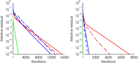
Fig. 1: Convergence of restarted GMRES applied to the original system with (dashed) and without (solid) deflation of the largest eigenvalues for three physically distinct scatterers. Deflation accelerates GMRES in the TM case (right), but does not work in the TE case (left). lossless object – red lines, object with small losses and negative real part of permittivity – green lines, and inhomogeneous object – blue lines.

Both the system matrix and the original integral operator are neither symmetric nor normal. Therefore, the range of iterative methods applicable to the problem is extremely limited, with (restarted) GMRES typically showing the best performance. Figure 1 shows the GMRES convergence histories on the original system $Au=b$ for three physically distinct scatterers (all with $\chi_{\rm m}=0$) and two different polarizations, corresponding to the TE and TM cases. The three scatterers are: a lossless object with large positive real permittivity, $\varepsilon/\varepsilon_{\rm b}=16$, an object with small losses and a large negative real part of the permittivity, $\varepsilon/\varepsilon_{\rm b}=-16+i1.5$, and an inhomogeneous object consisting of two concentric layers with the inner part having large losses, $\varepsilon/\varepsilon_{\rm b}=2.5+i20$, and the outer layer having a large positive real permittivity, $\varepsilon/\varepsilon_{\rm b}=16$. All objects are cylinders with square cross-sections with the side length $a=\lambda_{\rm b}$. The inner core of the inhomogeneous object has also a square cross-section with the side length $a/2$. The restart parameter of the GMRES algorithm is equal to $40$ (we shall study the influence of this parameter in more detail later). In Figure 1 (left) we illuminate the scatterers with a plane wave whose electric field vector is orthogonal to the axis of the cylinder (TE), whereas in Figure 1(right) the electric field vector of the incident plane wave is parallel to the axis of the cylinder (TM). Since all three objects do not exhibit any magnetic contrast with respect to the background medium, the integral operators are different for these TE and TM cases – see (9), (10). The latter contains now only the weakly singular part and is, therefore, of the form ‘identity plus compact’.

Next to the convergence plots of the original system in Figure 1 we present the convergence histories of the restarted GMRES with a deflation-based right preconditioner (dashed lines). As was suggested in [24], deflating the largest eigenvalues of $A$ in the TM case may significantly accelerate the convergence of the full (un-restarted) GMRES. The preconditioner deflating $r$ largest eigenvalues of $A$ is constructed by first running the eigs algorithm to retrieve these $r$ eigenvalues and the corresponding eigenvectors. With the help of the modified Gramm-Schmidt algorithm we further build an orthonormal basis for the retrieved set of eigenvectors. Let this basis be stored in a $3N\times r$ matrix $V$. Then, the right preconditioner [8] has the form

$$P^{-1}=I_{3N}+V\left[T^{-1}-I_{r}\right]V^{\ast},$$ (47)

with

$$T=V^{\ast}AV.$$ (48)

As was observed in [24] for the TM case, although the system matrix is not normal, the matrix $V$ has full column rank, and the matrix $T$ has a decent condition number. We confirm this behavior in the present TE case. The term ‘deflation’ refers to the fact that the spectrum of $AP^{-1}$ looks like the spectrum of $A$ with $r$ largest eigenvalues moved to the point $1+i0$ of the complex plane, and the corresponding eigen-subspace has been projected out. Here, even with the restarted GMRES, we see some improvement in the TM case Figure 1(right). The TE case, however, is not affected by deflation (it may even become worse).

Table 1 and Table 2 summarize the numerical results corresponding to the test objects in the TM and TE cases.

Table 1: Restarted GMRES with fair memory usage for three different test scatterers, TM case. Original and deflated systems.

		$r$, deflated		CPU time,	Iterations,	Speed-
System	$\varepsilon/\varepsilon_{\rm b}$	eigenvalues	restart	seconds	tol. $10^{-8}$	up
$A$	16	0	40	168	7311	1.0
$AP^{-1}$	16	28	12	78	4230	2.2
$A$	$-16+i1.5$	0	40	0.7	27	1.0
$AP^{-1}$	$-16+i1.5$	28	12	0.5	14	1.4
$A$	$16$ and $2.5+i20$	0	40	23	1000	1.0
$AP^{-1}$	$16$ and $2.5+i20$	28	12	14	749	1.6

The $3N\times r$ matrix $V$ needs to be stored in the memory. For the sake of fair comparison, we divide our memory between the inner Krylov subspace of the restarted GMRES and $V$, i.e., if we set ${\tt restart}=k$, $k>r$ with the original matrix $A$, then we use ${\tt restart}=k-r$ with the preconditioned matrix $AP^{-1}$.

(a) TE case.

(b) TM case.

Fig. 2: Eigenvalues of the system matrix $A$ for three physically distinct scatterers in the TE (top) and TM (bottom) cases. Horizontal axis – real part, vertical axis – imaginary part. Also shown (squares, triangles and circles) the values of the relative permittivity, including the background medium, in each scattering configuration.

One can understand the peculiar lack of progress in the TE case by considering Figure 2, which shows the spectra of the system matrix for the TE and TM cases corresponding to the numerical experiments of Figure 1. As can be seen, the difference between the spectra is in the presence of dence line segments $[1,\varepsilon(\mathbf{x})/\varepsilon_{\rm b}]$, $\mathbf{x}\in{\mathbb{R}}^{2}$ and some extra isolated eigenvalues inside a distribution remotely resembling a shifted circumference (the latter is much more pronounced with homogeneous objects at higher frequencies, see [24]). The dense line segments in the TE spectrum contain a very large number of closely spaced eigenvalues, and the deflation process simply stagnates when it reaches the outer ends of these lines, corresponding to $\varepsilon(\mathbf{x})/\varepsilon_{\rm b}$, $\mathbf{x}\in D$. Indeed, in the TE case we have seen no change in the convergence with $AP^{-1}$ when we tried to deflate any eigenvalues beyond those that were present outside a circle with the center at zero and the radius reaching the largest value of $|\varepsilon(\mathbf{x})/\varepsilon_{\rm b}|$, $\mathbf{x}\in{\mathbb{R}}^{2}$ for each particular scattering configuration. At the same time in the TM case we observed consistent improvement in convergence when deflating all eigenvalues outside the unit circle, see Table 1.

5 Preconditioning

In the three-dimensional case it was conjectured [4] that the dense line segments, which we now observe in the TE spectrum as well, are the discrete image of the essential spectrum, $\lambda_{\rm ess}=\varepsilon(\mathbf{x})/\varepsilon_{\rm b}$, of the corresponding singular integral operator. The absence of these lines in the TM spectrum is just another indirect confirmation. Yet, we do not have a formal proof, since there is no such thing as essential spectrum with matrices, and its role and transformation in the process of discretization is unclear. Anyway, the process of deflation is obviously hindered by those dense line segments and, assuming that they are due to the essential spectrum, we already know how to ‘deflate’ them. On the continuous level this can be achieved by regularization. We shall, therefore, apply the discretized regularizer $A_{\rm R}$, i.e., a discrete version of the operator $A(\chi^{\prime}_{\rm e})$, so that the problem becomes $A_{\rm R}Au=A_{\rm R}b$. Notice that no additional storage is required, since the original Green’s tensor can be re-used. Matrix-vector products, however, do become twice more expensive to compute.

To see how this procedure affects the matrix spectrum we compute the eigenvalues of $A_{\rm R}A$ corresponding to the matrices analyzed in Figure 2 (top). The results are presented in Figure 3, where we see that the line segments have been substantially reduced.

Fig. 3: Eigenvalues of the regularized matrix $A_{\rm R}A$, corresponding to the spectra of $A$ in the TE case, see Figure 2 (top). Red circles show the estimated outer bounds of the dense cluster – deflation bounds.

For a homogeneous object we can see what is going on also on the matrix level. The general form of our system matrix is $A=I-GX$, where $I$ is a $3N\times 3N$ identity matrix, $X$ is the diagonal matrix, containing the grid values of the contrast function, and $G$ is a dense matrix produced by the integral operator with the Green’s tensor kernel. When the contrast is homogeneous and equal to a scalar complex value $\chi=\varepsilon/\varepsilon_{\rm b}-1$ inside the scatterer, we can write our matrix as $A=I-\chi G$. Now, let $\psi_{n}$ be an eigenvector of $G$, i.e. $G\psi_{n}=\beta_{n}\psi_{n}$. Then, the eigenvalues of $A$ are:

$$\lambda_{n}=1-\beta_{n}\left(\frac{\varepsilon}{\varepsilon_{\rm b}}-1\right),$$ (49)

and the eigenvalues of $A_{\rm R}A$ are

$$\lambda^{\prime}_{n}=\left[1-\beta_{n}\left(\frac{\varepsilon_{\rm b}}{\varepsilon}-1\right)\right]\lambda_{n}.$$ (50)

Eliminating $\beta_{n}$ we get

$$\lambda^{\prime}_{n}=\left[1+\frac{\varepsilon_{\rm b}}{\varepsilon}(1-\lambda_{n})\right]\lambda_{n}.$$ (51)

We have verified numerically that this transformation holds for the first two plots of Figure 2 (top) and Figure 3. Curiously, the seemingly quadratic amplification of the large eigenvalues in (51) is moderated by the inverse of the relative permittivity. That is why the regularized spectra are not as extended as one would fear. Unfortunately, such a simple proof is not possible with an inhomogeneous object, yet the effect of the regularization on the matrix spectrum in Figure 2 (top, right) and Figure 3 (right) is obviously similar to the homogeneous cases.

Table 2 shows that such a regularized system is already better than the original one in terms of convergence. The relative speed-up, however, is limited to approximately $2.5$ times due to the extra work involved in computing the matrix-vector products with $A_{\rm R}A$. Moreover, no convergence improvement is observed with the negative permittivity object.

To further accelerate the convergence and make the method work with the negative permittivity objects as well (they are important in surface plasmon-polariton studies) we can now apply the deflation technique. For that we need to decide on the number of eigenvalues to be deflated. Obviously, it does not make sense to deflate beyond the first (from outside) dense cluster – deflation will only cost more time and memory, while the improvement will stagnate. After the regularization, the outer boundaries of the dense line segments have been all shifted inwards. However, due to nonlinear nature of the mapping (51) it is hard to tell exactly what an image of an arbitrary line segment would look like. Only for a lossless homogeneous scatterer are we able to predict that a real line segment $[1,\varepsilon/\varepsilon_{\rm b}]$ will be mapped onto the real line segment $[1,1+(1-\varepsilon/\varepsilon_{\rm b})^{2}/(4\varepsilon/\varepsilon_{\rm b})]$, which contracts the original segment by approximately four times. For a general line segment radially emerging from the point $1+i0$ we have made a small numerical routine, which produces a discretized image according to (51) and finds the point with the largest absolute value – the radius of the circle beyond which all eigenvalues should be deflated. We have observed, by analyzing the spectra for various inhomogeneous objects, that the general regularization seems to transform each line segment according to (51). Therefore, in an inhomogeneous case, we can simply apply the aforementioned numerical mapping to each of the segments $[1,\varepsilon(\mathbf{x})/\varepsilon_{b}]$, $\mathbf{x}\in D$, and choose the point with the maximum absolute value as the deflation radius. The deflation bounds obtained in this way are shown in Figure 3 as solid red circles.

The number of eigenvalues outside the deflation bound depends on the physics of the problem. For example, we know that at low frequencies (large wavelengths) all discrete eigenvalues are located within the convex hull of the essential spectrum [3], and that at higher frequencies they tend to spread out. We have investigated this phenomenon in more detail and have found a pattern, similar to the one reported in [24]. As one can see from Figure 4 (left), the ratio of the number $r$ of eigenvalues outside the

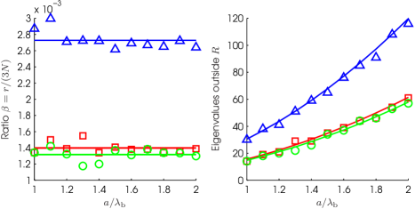
Fig. 4: Dependence of the number of eigenvalues to be deflated on the wavelength for three test scatterers (same medium parameters as in previous figures). Left: ratio $\beta$ of the number $r$ of eigenvalues outside the deflation bound (circles with radius $R$, see Figure 3) to the total number $3N(\lambda_{\rm b})$ of eigenvalues for a classical discretization rule (fixed number of points per smallest medium wavelength). Right: actual number $r$ of eigenvalues to be deflated (with magnitude greater than the deflation bound $R$) and our analytical prediction based on an average $\beta$ coefficient estimated from the left plot.

deflation bound to the total number of eigenvalues $3N$ is roughly constant (for objects larger than $\lambda_{\rm b}$), if at each wavelength we adjust the spatial discretization according to the classical rule (say, $15$ points per smallest medium wavelength). Hence, with fixed medium parameters and a square computational domain with side $a$, the total number of unknowns and therefore eigenvalues grows as $3N=3[\alpha^{2}(a/\lambda_{\rm b})^{2}+2\alpha(a/\lambda_{\rm b})+1]$ with $\alpha=15\max\{\sqrt{(\varepsilon^{\prime}/\varepsilon_{\rm b})}\}$. Thus, knowing $\beta=r/(3N)$ for some wavelength, we can estimate $r=3N\beta$ at any other wavelength. This empirical law comes very handy since solving a relatively low-frequency spectral problem can be really easy due to small system matrix dimensions. Otherwise, if there is no shortage of memory for the chosen wavelength, one can simply run the eigs routine increasing the number of recovered largest eigenvalues until the deflation bound obtained above is reached.

Having a good estimate of the deflation parameter $r$ we have applied the right preconditioner given by (47) to the regularized system for the same three objects as in all previous examples. The largest eigenvalues/eigenvectors of the regularized system turn out to be very stable, so that one can safely apply the eigs routine with its tolerance set as high as $10^{-2}$. Though, we have not seen any substantial acceleration beyond the $10^{-4}$ tolerance, which, in its turn, gave us a significant speed-up in the off-line work compared to the default machine precision tolerance. In all our experiments, the off-line time remained a small fraction of the total CPU time (for concrete numbers we refer to the example at the end of this Section).

The convergence histories for a restarted GMRES with this preconditioner are presented in Figure 5.

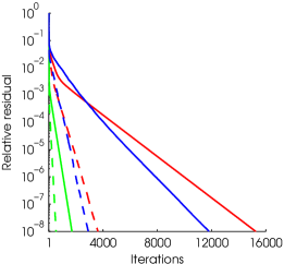
Fig. 5: Convergence of restarted GMRES with the original $Au=b$ (solid) and preconditioned $A_{\rm R}AP^{-1}v=A_{\rm R}b$ (dashed) systems for the three physically distinct scatterers in the TE case. Red lines; $\varepsilon/\varepsilon_{\rm b}=16$; Green lines: $\varepsilon/\varepsilon_{\rm b}=-16+i1.5$; Blue lines: inhomogeneous object $\varepsilon/\varepsilon_{\rm b}=(16,2.5+i20)$.

Table 2: Restarted GMRES with fair memory usage for three different test scatterers, TE case. Original, deflated, regularized, and regularized-plus-delfated systems.

		$r$, deflated		CPU time,	Iterations,	Speed-
System	$\varepsilon/\varepsilon_{\rm b}$	eigenvalues	restart	seconds	tol. $10^{-8}$	up
$A$	16	0	40	350	15258	1.0
$AP^{-1}$	16	6	34	306	14002	1.1
$A_{\rm R}A$	16	0	40	142	4030	2.5
$A_{\rm R}AP^{-1}$	16	14	26	117	3626	3
$A$	$-16+i1.5$	0	40	39	1708	1.0
$AP^{-1}$	$-16+i1.5$	7	33	36	1659	1.1
$A_{\rm R}A$	$-16+i1.5$	0	40	36	1021	1.1
$A_{\rm R}AP^{-1}$	$-16+i1.5$	30	10	16	534	2.4
$A$	$16$ and $2.5+i20$	0	40	275	11823	1.0
$AP^{-1}$	$16$ and $2.5+i20$	3	37	310	13156	0.9
$A_{\rm R}A$	$16$ and $2.5+i20$	0	40	107	3032	2.6
$A_{\rm R}AP^{-1}$	$16$ and $2.5+i20$	14	26	94	2911	3

This figure, and the iteration counts in general, are slightly misleading when one deals with an iterative algorithm like restarted GMRES. For example, we see in Table 2 that, apart from the negative permittivity case, the iteration counts after deflation are only slightly better than what we have already achieved with the regularized system. Hence, one could conclude that the deflation is not worth the effort. However, the GMRES algorithm does not scale lineraly in time as a function of the restart parameter, i.e., while it may converge in less iterations for larger values of restart, the CPU time may not decrease as much. This has partly to do with the re-orthogonalization process, which takes more time for larger inner Krylov subspaces, and partly with the very bad spectral properties of our system matrix.

Thus, to decide upon the benefits of deflation we compare execution times for various values of restart parameter. In addition, we need to consider another important constraint – the available memory. Since a fair comparison can only be achieved if we give the same amount of memory to both the original and the preconditioned systems, we give all the available memory to the GMRES algorithm in the former case, and split it between the restart and the deflation subspace of size $r$ in the latter. Finally, we want to know if the efficiency of the proposed preconditioner depends on the physics of the problem, i.e., does it work better or worth for larger objects and contrasts? Of course, the system becomes larger and more difficult to solve for larger objects, and we have to be prepared to increase the value of restart for larger objects and contrasts to achieve any convergence at all. Hence, assuming that we have enough memory at least for deflation, we shall distinguish between the following three situations: limited memory, ${\tt restart}(A_{\rm R}AP^{-1})<r$; moderate memory, ${\tt restart}(A_{\rm R}AP^{-1})\sim r$; large memory, ${\tt restart}(A_{\rm R}AP^{-1})>r$.

We observe from the plots of Figure 6 that with limited memory, where we choose ${\tt restart}(A_{\rm R}AP^{-1})=r/2$ and ${\tt restart}(A)=r$, the original system initially outperforms the preconditioned one. As the object size grows, so does the size $r$ of the deflation subspace. Since in that case the ${\tt restart}(A_{\rm R}AP^{-1})$ parameter grows as well, at some point (for $a/\lambda=1.9$ with this particular object) it reaches a value at which the preconditioned system breaks even and begins to outperform the original one for larger objects (maximum achieved speed-up is $2.4$ times at $a/\lambda_{\rm b}=2.2$). With moderate memory, ${\tt restart}(A_{\rm R}AP^{-1})=2r$, ${\tt restart}(A)=3r$, the preconditined system always performs better than the original one. Moreover, the relative speed-up Figure 6 (right) generally increases with the object size (maximum achieved speed-up is $5.1$ times at $a/\lambda_{\rm b}=2$, minimum – $2.1$ times at $a/\lambda_{\rm b}=1$). With large memory, i.e., for ${\tt restart}(A_{\rm R}AP^{-1})=10r$ and ${\tt restart}(A)=11r$, the speed-up may be as high as $46.6$ times ($a/\lambda_{\rm b}=2.2$) (minimum speed-up of $8.7$ times at $a/\lambda_{\rm b}=1$), and it also grows (on average) with the object size.

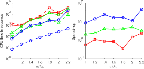
Fig. 6: CPU time (left) and the achieved speed-up (right) as a function of wavelength (object size) for ${\tt restart}=r/2$ (red, squares), ${\tt restart}=2r$ (green, triangles), and ${\tt restart}=10r$ (blue, circles). The permittivty of the scatterer is $\varepsilon/\varepsilon_{\rm b}=16$. Solid lines – original system $Au=b$; dashed lines – preconditioned system $A_{\rm R}AP^{-1}v=A_{\rm R}b$.

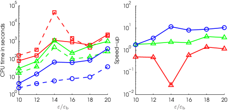
Fig. 7: CPU time (left) and the achieved speed-up (right) as a function of permittivity for ${\tt restart}=r/2$ (red, squares), ${\tt restart}=2r$ (green, triangles), and ${\tt restart}=10r$ (blue, circles). The scatterer is lossless with side length fixed at $a/\lambda_{\rm b}=1$. Solid lines – original system $Au=b$; dashed lines – preconditioned system $A_{\rm R}AP^{-1}v=A_{\rm R}b$.

With objects of finite extent changing the wavelength of the incident field is not the same as changing the object permittivity. Hence, we repeat the same numerical experiments as in Figure 7, but now for an object of fixed size, $a/\lambda_{\rm b}=1$, and varying permittivity. The deflation parameter $r$ is estimated using the same algorithm as above and turns out to grow only slightly as a function of permittivity, climbing from $13$ to $17$ for the permittivity changing between $10$ and $20$. At the same time the total number of unknowns as well as eigenvalues grows very fast. Therefore, deflation did not accelerate the iterative process here as much as when we changed the wavelength, and most of the speed-up must be due to the regularization. For this relatively small scatterer we see some improvement in convergence only with relatively large amounts of memory devoted to the restart parameter, i.e., ${\tt restart}(A_{\rm R}AP^{-1})\geq 2r$. Moreover, preconditioned GMRES with ${\tt restart}(A_{\rm R}AP^{-1})=r/2$ did not converge for $\varepsilon/\varepsilon_{\rm b}=14$ at all (we set this point arbitrarilly high in the plot). On the other hand, the maximum speed-up for ${\tt restart}=2r$ was $4.1$ times (ninimum $1.8$ times), while for ${\tt restart}=10r$ the maximum speed-up was $11.4$ times (minimum $1.6$ times). From the previous experiments we may expect that the speed-up will be larger with larger objects.

As an example of a systematic application of the present preconditioner, we consider the problem, for which the DIE method is most suited, i.e., scattering on an object with continuously varying permittivity. The steps we suggest to follow are:

1. Determine the total available memory: $M$ bytes

2. Fix the discretization rule at $k$ points per smallest medium wavelength.

3. Estimate $\beta$ from low-frequency matrix spectra.

4. Determine the maximal number of grid points $N_{\rm max}$:

   • If $a$ – size of the computational domain $D$, and $N$ – number of grid points, then $N=\alpha^{2}(a/\lambda_{\rm b})^{2}+2\alpha(a/\lambda_{\rm b})+1$, where
     $\alpha=k\max\{\sqrt{(\varepsilon^{\prime}(\mathbf{x})/\varepsilon_{\rm b})}\}$, $\mathbf{x}\in D$.

   • Memory needed for the system, right-hand side, and the unknown vector: $M_{A}=720N$ bytes (one complex number – 16 bytes).

   • Memory required for deflation and GMRES:
     $M_{\rm Prec}=16r^{2}+48Nr+48N{\tt restart}$ bytes, where $r=3N\beta$ and
     ${\tt restart}=xr$, i.e., $M_{\rm Prec}=144(\beta^{2}+\beta+x\beta)N^{2}$ bytes.

   • The largest affordable grid follows from $M_{A}+M_{\rm Prec}\approx M$:
     $N_{\rm max}\approx[\sqrt{900+M(\beta^{2}+\beta+x\beta)}-30]/[12(\beta^{2}+\beta+x\beta)]$.

5. Determine the maximum affordable object size (smallest wavelength) via $[a/\lambda_{\rm b}]_{\rm max}=(\sqrt{N_{\rm max}}-1)/\alpha$.

The scatterer is depicted in Figure 8 (left). The relative permittivity function profile is given by

$$\varepsilon(\mathbf{x})/\varepsilon_{\rm b}=10+5\sin(4\pi x_{1}/a)\sin(4\pi x_{2}/a),$$ (52)

where the origin of the coordinate system is in the middle of the computational domain. We calculated $\beta$ for this scatterer to be approximately $0.0011$. Having $M=4$ GB of memory available and choosing $k=15$ and ${\tt restart}(A_{\rm R}AP^{-1})=8r$, from the above algorithm we determine the largest affordable size with this permittivity as $[a/\lambda_{\rm b}]_{\rm max}=4$. Hence, the total number of unknowns is $3N=162867$ and the deflation parameter is $r=180$. The GMRES was restarted at ${\tt restart}(A_{\rm R}AP^{-1})=1440$ and ${\tt restart}(A)=1620$. The results of this test are as follows: original system – $162692$ seconds of CPU time, preconditioned system – $11620$ seconds. The speed-up in pure ‘on-line’ calculations is $14$ times, as we would expect from our previous experiments with the homogeneous test object. The off-line work with the tolerance of eigs set to $10^{-4}$ took only $775$ seconds, so that even with this time included we get a $13.1$ times speed-up. The computed electric field is shown in Figure 8 (right).

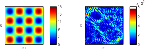
Fig. 8: Scattering of a TE plane wave on an inhomogeneous object with continuously varying permittivity. Left – permittivity profile (side length $a/\lambda_{\rm b}=4$). Right – computed electric field intensity $|E_{1}|^{2}+|E_{2}|^{2}$. Preconditioning gives $14$ times speed-up for this problem.

The CPU timing is provided here merely for illustration and should not be used for direct comparison against the local methods, which was not the purpose of this paper either. For the particular problems considered above one could, for instance, substantially accelerate the calculations and free some valuable memory by computing the electric field only. On the other hand, the presented CPU timing data give us a good relative estimate of what to expect with objects having both electric and magnetic contrasts so that both electric and magnetic fields must indeed be computed at the same time.

Finally we should mention that, while we have been focusing here on the restarted GMRES, obviously, any other memory-efficient solver, which works with the original system $Au=b$, could also be applied to the preconditioned system $A_{\rm R}AP^{-1}v=A_{\rm R}b$. We have considered, for instance, Bi-CGSTAB, restarted GCR, and IDR. Sometimes we could achieve faster convergence by tuning the restart method of GCR, although, this did not happen with all types of scatterers (only with a homogeneous lossless one). Moreover, with some scatterers (inhomogeneous with losses) GCR and other algorithms would simply stagnate. Thus, for the moment, the restarted GMRES remains the most robust solver for the present problem, whereas other algorithms require more tuning and a more systematic study.

6 Conclusions

The analysis of the domain integral operator of the transverse electric scattering presented here helps to understand the reasons behind the extremely slow convergence of iterative methods often observed with this method. Unlike the TM case, which is equivalent to the Helmholtz equation and can be easily accelerated by deflating the largest eigenvalues, the TE case showed no improvement with this type of preconditioner. Direct numerical comparison of the TE and TM matrix spectra indicates that the nontrivial essential spectrum of the TE operator results in extended and very dense eigenvalue clusters, that cause stagnation of the deflation process with high-contrast objects. We have derived an analytical multiplicative regularizer and demonstrated on various test scatterers that its discretized version robustly reduces the extent of the troublesome dense clusters. One can view the obtained regularizer as a generalization of the Calderón identity, previously applied in the preconditioning of boundary integral equations. Notably, the discretized regularizer does not require any extra computer memory and its action on a vector can be computed at FFT speed. Applying deflation of the largest-magnitude eigenvalues on the regularized system we could achieve up to $46.6$ times acceleration of the restarted GMRES with relatively large memory, and up to $5.1$ times with modest memory. The off-line work typically takes only a small fraction of the total time, since one can apply a very rough tolerance in the eigs algorithm when recovering the largest-magnitude eigenvalues/eigenvectors. Somewhat surprisingly, this preconditioner showed a tendency to become more efficient (on average) with the increase in the object size and permittivity.

References

- [1] F. P. Andriulli, K. Cools, H. Bağci, F. Olyslager, A. Buffa, S. Christiansen, and E. Michielssen, A multiplicative Calderón preconditioner for the electric field integral equation, IEEE Transactions on Antennas and Propagation, 56 (2008), pp. 2398–2412.
- [2] H. Bağci, F. P. Andriulli, K. Cools, H. Bağci, F. Olyslager, and E. Michielssen, A Calderón multiplicative preconditioner for coupled surface-volume electric field integral equations, IEEE Transactions on Antennas and Propagation, 58 (2010), pp. 2680–2690.
- [3] N. V. Budko, A.B. Samokhin, and A.A. Samokhin, A generalized overrelaxation method for solving singular volume integral equations in low-frequency scattering problems, Differential Equations, 41 (2005), pp. 1262–1266.
- [4] N. V. Budko and A. B. Samokhin, Spectrum of the volume integral operator of electromagnetic scattering, SIAM J. Sci. Comp., 28 (2006), pp. 628–700.
- [5] M. Card, M. Bleszynskiz, and J. L. Volakis, A near-field preconditioner and its performance in conjunction with the BiCGstab(l) solver, IEEE Antennas and Propagation Magazine, 46 (2004), pp. 23–30.
- [6] S. H. Christiansen and J.-C. Nedelec, A preconditioner for the electric field integral equation based on Calderón formulas, SIAM J. Numer. Anal., 40 (2003), pp. 1100–1135.
- [7] R. Coifman, V. Rokhlin, and S. Wandzura, The fast multipole method for the wave equation: A pedestrian prescription, IEEE Antennas and Propagation Magazine, 35 (1993), pp. 7–12.
- [8] J. Erhel, K. Burrage, and B. Pohl, Restarted GMRES preconditioned by deflation, J. Com. App. Math., 69 (1996), pp. 303–318.
- [9] Y. A. Erlangga, Advances in iterative methods and preconditioners for the Helmholtz equation, Arch. Comput. Methods Eng., 15 (2008), pp. 37–66.
- [10] Y. A. Erlangga, C. W. Oosterlee, and C. Vuik, A novel multigrid based preconditioner for heterogeneous Helmholtz problems, SIAM J. Sci. Comp., 27 (2006), pp. 1471–1492.
- [11] Z. H. Fan, D. X. Wang, R. S. Chen, and E. K. N. Yung, The application of iterative solvers in discrete dipole approximation method for computing electromagnetic scattering, Microwave Opt. Tech. Lett., 48 (2006), pp. 1741–1746.
- [12] P. J. Flatau, Improvements in the discrete-dipole approximation method of computing scattering and absorption, Optics Letters, 22 (1997), pp. 1205–1207.
- [13] R. F. Harrington, Field Computation by Moment Method, IEEE press, Piscataway, NJ, 1993.
- [14] F. Ihlenburg and I. Babuska, Dispersion analysis and error estimation of Galerkin finite element methods for the helmholtz equation, Int. J. Numer. Methods Eng., 38 (1995), pp. 3745–3774.
- [15] , Finite element solution of the Helmholtz equation with high wave number. Part I: the h-version of the FEM, Comput. Math. Appl., 30 (1995), pp. 9–37.
- [16] A. S. Ilinski, A. B. Samokhin, and U. U. Kapustin, Mathematical modelling of 2D electromagnetic scattering, Computers and Mathematics with Applications, 40 (2000), pp. 1363–1373.
- [17] N. Joachimowicz and C. Pichot, Comparison of three integral formulations for the 2-D TE scattering problem, IEEE Transactions on Microwave Theory and Techniques, 38 (1990), pp. 178–185.
- [18] R. E. Kleinman, G. F. Roach, and P. M. van den Berg, Convergent Born series for large refractive indices, Journal of the Optical Society of America, 7 (1990), pp. 890–897.
- [19] D. E. Livesay and K.-M. Chen, Electromagnetic fields induced inside arbitrarilly shaped biological bodies, IEEE Transactions on Microwave Theory and Techniques, 22 (1974), pp. 1273–1280.
- [20] S. G. Mikhlin and S. Prössdorf, Singular Integral Operators, Springer-Verlag, Berlin, 1986.
- [21] A. F. Peterson and P. W. Klock, An improved MFIE formulation for TE-wave scattering from lossy, inhomogeneous dielectric cylinders, IEEE Transactions on Antennas and Propagation, 36 (1988), pp. 45–49.
- [22] J. H. Richmond, TE-wave scattering by a dielectric cylinder of arbitrary cross-section shape, IEEE Transactions on Antennas and Propagation, 14 (1966), pp. 460–464.
- [23] A. B. Samokhin, Integral Equations and Iteration Methods in Electromagnetic Scattering, VSP, Utrecht, The Netherlands, 2001.
- [24] J. Sifuentes, Preconditioning the integral formulation of the Helmholtz equation via deflation, master’s thesis, Applied Mathematics, Rice University, Houston, Texas, 2006. Online at: http://scholarship.rice.edu/handle/1911/17917.
- [25] T. Søndergaard, Modeling of plasmonic nanostructures: Green’s function integral equation methods, Phys. Stat. Sol., 244 (2007), pp. 3448–3462.
- [26] J. M. Song, C.-C. Lu, and W. C. Chew, Multilevel fast multipole algorithm for electromagnetic scattering by large complex objects, IEEE Transactions on Antennas and Propagation, 45 (1997), pp. 1488–1493.
- [27] C.-C. Su, A simple evaluation of some principal value integrals for dyadic Green’s function using symmetry property, IEEE Transactions on Antennas and Propagation, 35 (1987), pp. 1306–1307.
- [28] J. L. Volakis, Alternative field representations and integral equations for modeling inhomogeneous dielectrics, IEEE Transactions on Microwave Theory and Techniques, 40 (1992), pp. 604–608.
- [29] M. A. Yurkin and A.G. Hoekstra, The discrete dipole approximation: An overview and recent developments, Journal of Quantitative Spectroscopy and Radiative Transfer, 106 (2007), pp. 558–589.