¹ Department of Physics and Astronomy, Potsdam University, Karl-Liebknecht-Str. 24/25, D-14476, Potsdam-Golm, Germany
² Ambrosys GmbH, Geschwister-Scholl-Str. 63a, 14471 Potsdam, Germany
³ UP Transfer GmbH, Am Neuen Palais 10, 14469 Potsdam, Germany
^∗ Corresponding author, karsten.ahnert@ambrosys.de, Tel: +49 331 9775986
Major Subject: Physical sciences
Minor Subject: Applied Physical Sciences
Date:

Abstract

Wave energy harvesting could be a substantial renewable energy source without impact on the global climate and ecology, yet practical attempts have struggled with problems of wear and catastrophic failure. An innovative technology for ocean wave energy harvesting was recently proposed, based on the use of soft capacitors. This study presents a realistic theoretical and numerical model for the quantitative characterization of this harvesting method. Parameter regions with optimal behavior are found, and novel material descriptors are determined which simplify analysis dramatically. The characteristics of currently available material are evaluated, and found to merit a very conservative estimate of 10 years for raw material cost recovery.

I Introduction

The problem of adequately supplying the world with clean, renewable energy is among the most urgent today. It is crucial to evaluate alternatives to conventional techniques. One possibility is energy harvesting from ocean waves, which has been proposed as a means of offsetting a large portion of the world’s electrical energy demands Cruz-08 . However, the practical implementation of wave energy harvesting has met with obstacles, and the development of new methods is necessary Dalton2010 . Oceanic waves have large amplitude fluctuations that cause devices to fail due to excessive wear or during storms. A strategy to overcome these catastrophic events could be to base the harvesting mechanisms on soft materials.

Soft, stretchable rubber capacitors are possible candidates for energy harvesting  Pelrine2001 ; Jean-Mistral2008 ; Graf2010a ; Brochu2010 , that have already been tested in a realistic ocean setting Chiba2007 ; Chiba2008 . They were originally introduced as actuators Pelrine2000b ; Carpi2008 ; Brochu2010a ; Carpi24122010 , capable of high actuation strains of more than 100% and stresses of more than 1 MPa. With a soft capacitor, mechanical energy can be used to pump charges from a low electrical potential $U$ to a higher, such that the electrical energy difference can be harvested Pelrine2001 . This is made possible by the large changes of capacitance under mechanical deformation. Although the method is simple and proven Pelrine2001 ; Chiba2007 ; Chiba2008 ; Jean-Mistral2008 ; Graf2010a ; Brochu2010 , it is still not clear to which extent the approach is practically useful, which is the concern of this paper. Of the many electro-active polymers, it appears that soft capacitors could have the highest energy densities Jean-Mistral2010 .

For the purpose of a broad and realistic investigation, a minimal yet realistic model is proposed that takes into account the mechanical and dielectric properties of the soft capacitor material, including losses and limiting criteria. The model also includes cyclic mechanical driving, and an electrical control mechanism consisting of a switchable electrical circuit. The quality of the energy harvesting is characterized by efficiency and gain measures, which were evaluated for simulations on a very large set of varied system and material parameters.

The so far only commercially available soft capacitor material, DEAP (Danfoss PolyPower A/S), is used here as benchmark Benslimane2002 ; DanfossPolyPower ; Benslimane2010 . DEAP consists of a sheet of silicone elastomer with smart compliant metal electrodes and is a realistic candidate with adequate properties for energy harvesting Graf2010 . The high voltage required for operation of soft capacitor actuators has led to research efforts aiming at lowering the voltages by modifying their mechanical or dielectric properties. Preferably, they should have low mechanical stiffness and high dielectric constant, $\varepsilon_{r}$ Carpi2008a ; Molberg2010 ; Gallone2010 ; Stoyanov2010 ; StoyanovC0SM00715C . In general, the dielectric constant can be adjusted from 2 to more than 1000, however, at higher values such strategies usually cause excessive conductivity and premature electrical breakdown.

II The Model

The model describes the dynamics of the deformations of and the voltage across the soft capacitor. It includes mechanical and dielectric properties. Losses appear mainly electrically in the electrodes and in the charging and discharging circuits. The external force is sinusoidal and linearly coupled to the length of the soft capacitor; we regard these as minimum requirements for the description of coupling to near-coast oceanic surface waves. Technically, elaborate wave-capacitor coupling mechanisms are possible, yet here the focus is placed on the general principle. Mechanical conversion efficiency and electrical energy gain factors are calculated from time-integrated losses, mechanical input and electrical output.

The deformation of the polymer film is described in terms of the deformation ratios $\lambda_{i}=L_{i}/L_{i}^{\prime}$ (with $i=1,2,3$ for the $x,y,z$-axes), where $L_{i}$ and $L_{i}^{\prime}$ are the final and the initial dimensions, respectively. The electrical field is applied in $z$-direction and the mechanical driving force $f_{1}$ acts in $x$-direction. For elastomers, which are amorphous and non-crystalline, wolume conservation can be assumed, $\lambda_{1}\lambda_{2}\lambda_{3}=1$. Also, the pure shear condition is assumed, $\lambda_{2}=\text{constant}$.

The time-dependent mechanical response is chosen as a Kelvin-like fluid Brinson-Polymer-Book ,

$$T_{ii}=p+\frac{f_{i}}{A_{i}}-\gamma\dot{\lambda}_{i}\,\text{,}$$ (1)

which balances the internal material stress $T_{ii}$, the hydrostatic pressure $p$, the external forces $f_{i}$, and the viscous damping characterized by $\gamma$. Eliminating the pressure from both equations, utilizing the volume constraint ($\lambda_{3}=\lambda_{1}^{-1}$), and splitting the material stress into a mechanical and an electrical part Kofod2005 yields

$$-\gamma\dot{\lambda}_{1}=\left[\frac{\lambda_{1}^{2}}{\lambda_{1}^{2}+1}\right]\left(\sigma_{\rm Mech}+\sigma_{\rm Elec}-\frac{\lambda_{1}f_{1}}{L_{2}^{\prime}L_{3}^{\prime}}\right)\,\text{.}$$ (2)

For $\sigma_{\rm Mech}$, the Yeoh model Yeoh-93 is chosen, with parameters $C_{10}$, $C_{20}$, $C_{30}$:

$$\sigma_{\rm Mech}=2\left(\lambda_{1}^{2}-\lambda_{1}^{-2}\right)\left(C_{10}+2C_{20}\Lambda+3C_{30}\Lambda^{2}\right)\;,$$ (3)

where $\Lambda=\lambda_{1}^{2}+\lambda_{1}^{-2}-2$. The Young’s modulus of the Yeoh material under pure shear conditions is $Y=8C_{10}$.

The electrical part of the internal stress $\sigma_{\rm Elec}$, also known as Maxwell stress is $\sigma_{\rm Elec}=-\varepsilon_{r}\varepsilon_{0}E^{2}$, where $E=U/L_{3}$ is the electrical field between the electrodes Pelrine2000b ; Kofod2005 ; Suo2008 . It describes the stress due to the voltage difference $U$ between the capacitor electrodes. The permittivity of an elastomer does not change at the relatively low levels of electrical field encountered here, and it also does not change when it is deformed, as has been repeatedly verified experimentally by researchers Lillo2011 ; Kofod2005 .

The dynamics of the voltage between the electrodes can be derived from $Q=CU$, where $Q$ is its charge and $C$ the capacitance. Building the time derivative and rearranging this equation yields

$$\dot{U}=-\frac{\sigma_{\rm DC}}{\varepsilon_{0}\varepsilon_{r}}U+\frac{I_{\rm C}}{C^{\prime}\lambda_{1}^{2}}-2U\frac{\dot{\lambda}_{1}}{\lambda_{1}}\,\text{.}$$ (4)

The first term corresponds to leakage current due to the finite polymer conductivity $\sigma_{\rm DC}$, the second accounts for the electrical control circuit, and the third for mechanical deformation. $C^{\prime}=\varepsilon_{r}\varepsilon_{0}L_{1}^{\prime}L_{2}^{\prime}/L_{3}\prime$ is the capacitance of the unperturbed capacitor, and $C=C^{\prime}\lambda_{1}^{2}$ that of the deformed.

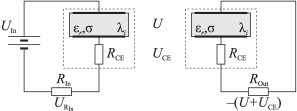
Figure 1: The electrical circuits. Left: charging process, right: discharging process.

Eqs. (2) and (4) define a system of two coupled ordinary differential equations (ODEs) for the stretch $\lambda$ and the voltage $U$. The only unknowns are the external driving force $f_{1}$ and the electrical current from the charging and discharging circuit. The force is chosen by a simple periodic driving $f_{1}=f_{0}+f_{\rm A}\sin(\omega t+\varphi)$, where the actual geometry of the pick-up mechanism can help in adjusting bias force $f_{0}$ and amplitude $f_{\rm A}$. The angular frequency $\omega=2\pi/t_{\rm C}$ is determined by the period of the oscillating force, $t_{\rm C}$.

A very simple charge and discharge control mechanism is chosen here. It is described by three points in time. The voltage is ramped on the soft capacitor at $t_{0}=0$, stopped at $t_{1}$, while discharging starts at $t_{2}$. The discharging process ends at $t_{C}$. A phase difference, $\varphi$, adjusts the onset of the control relative to the driving force.

The capacitor is charged during $(t_{0},t_{1})$ in an electrical circuit shown in Fig. 1. Kirchhoff’s laws state that $U_{\rm In}+U+U_{{\rm CE}}+U_{\rm R_{In}}=0$ and that $I_{\rm C}=\text{const}$. $U_{\rm In}$ is the driving voltage of the external voltage supply, $U_{{\rm CE}}$, and $U_{\rm R_{In}}$ are the voltage drops over the capacitor electrodes and the charging resistor, with resistance $R_{\rm CE}$ and $R_{\rm In}$. This yields the current

$$I_{\rm C}=-\frac{U_{\rm In}+U}{R_{\rm CE}+R_{\rm In}}\,\text{.}$$ (5)

which follows the voltage ramp $U_{\rm In}(t)=\frac{t}{t_{1}}U_{\rm In,max}$, where $U_{\rm In,max}$ is the maximal charging voltage.

In the interval $(t_{1},t_{2})$ the circuit is detached. Mechanical deformation and variation in voltage takes place due to the external variation in force. The response is influenced by viscoelastic damping, while current leakage leads to partial charge loss.

During $(t_{2},t_{C})$ the discharging electrical circuit is attached, cf. Fig. 1. Now, no external voltage is applied and the discharging resistor $R_{\rm Out}$ is used:

$$I_{\rm C}=-\frac{U}{R_{\rm CE}+R_{\rm Out}}\,\text{.}$$ (6)

After discharging the cycle starts over.

In the ODEs (2) and (4) four relaxation processes with different time scales are given: one mechanical, $\tau_{M}$, two electrical, $\tau_{C}$ and $\tau_{D}$, and $\tau_{\rm PC}$ describing the loss of charge through the polymer material. In addition, there is the period of the driving, $t_{C}$. The mechanical relaxation of the polymer to an equilibrium state $\lambda_{1}^{\star}$ is described by $\tau_{M}^{-1}=\mbox{d}F(\lambda_{1})/\mbox{d}\lambda_{1}|_{\lambda_{1}^{\star}}$. $F(\lambda)$ is given by (2) via $\dot{\lambda}_{1}=F(\lambda_{1})$. For the Yeoh model this time scale is approximately $\tau_{M}=0.55\,\mathrm{s}$. The electrical relaxation time scales during charging and discharging are $\tau_{C}=(R_{\rm CE}+R_{\rm In})C$ and $\tau_{D}=(R_{\rm CE}+R_{\rm Out})C$. They are typically in the order of $10^{-5}\,\mathrm{s}$. The largest time scale, which we term the Maxwell time, describes the loss of charge through the polymer material $\tau_{\rm PC}=\frac{\varepsilon_{0}\varepsilon_{r}}{\sigma_{\rm DC}}$.

Material failure sets limits which are monitored during simulations and which have been taken into account: i) $\lambda_{1}<5$ avoids rupture, ii) $T_{11}>0$ ensures a taut material, iii) $E=\frac{U}{L_{3}}<20\,\mathrm{\frac{V}{m}}$ avoids intrinsic electrical breakdown, and iv) $\frac{\varepsilon_{0}\varepsilon_{r}V^{2}}{(L_{3}^{\prime})^{2}}\lambda_{1}^{4}<H(\lambda_{1})$ avoids the the electromechanical instability, analogous to pull-in failure Zhao2007 ; H-Formula .

Table 1: Default parameters for energy harvesting simulations.

Material and capacitor parameters
$L_{1}^{\prime}$, $L_{2}^{\prime}$, $L_{3}^{\prime}$	$0.1\,\mathrm{m}$, $0.2\,\mathrm{m}$, $5\cdot 10^{-5}\,\mathrm{m}$
$C_{10}$, $C_{20}$, $C_{30}$	$139840\,\mathrm{Pa}$, $-6570\,\mathrm{Pa}$, $1057\,\mathrm{Pa}$
$\varepsilon_{r}$	$3.1\,\mathrm{}$
$\sigma_{\rm DC}$	$10^{-13}\,\mathrm{\frac{A}{Vm}}$
$R_{\rm CE}$	$1000\,\mathrm{\Omega}$
$\gamma$	$10^{6}\,\mathrm{s/Pa}$
Driving parameters
$f_{A}=1\,\mathrm{N}$, $f_{0}=2\,\mathrm{N}$, $t_{C}=10\,\mathrm{s}$
Circuit parameters
$U_{\rm In,Max}$	$651\,\mathrm{V}$
$R_{\rm In}$, $R_{\rm Out}$	$10^{6}\,\mathrm{\Omega}$, $3.83\cdot 10^{7}\,\mathrm{\Omega}$
$t_{1}$, $t_{2}$, $t_{C}=2\pi/\omega$
Limiting parameters
$\lambda_{\rm Max}$	$5$
$E_{\rm Max}$	$20\,\mathrm{Vm^{-1}}$

The mechanical work is generally defined as $W=L_{1}^{\prime}\int f(\lambda_{1},t)\dot{\lambda}_{1}\mbox{d}t$, where $f(\lambda,t)$ is an arbitrary force acting on the film. Using this equation and writing all terms in Eq. (2) as forces allows the calculation of the work, for example $W_{\rm Mech}=L_{1}^{\prime}\int A_{1}\sigma_{\rm Mech}\dot{\lambda}_{1}\mbox{d}t$. Energy is conserved over one cycle, hence $W_{\rm Visco}+W_{\rm Driving}=W_{\rm Mech}+W_{\rm Maxwell}$. The electrical work is similarly $W=\int UI\mbox{d}t$; again, several contributions should be evaluated. Energy conservation leads to $W_{\rm Capacitor}+W_{\rm U,In}+W_{\rm R,In}+W_{\rm R,CE}=0$ for the charging, and to $W_{\rm Capacitor}+W_{\rm R,Out}+W_{\rm R,CE}=0$ for the discharging. It is emphasized that the definition of the voltage allows for negative or positive values for the work done.

The quality of the harvesting process is evaluated by the harvesting efficiency $\eta$ and the gain $G$. The efficiency $\eta$ is the ratio of electrical output energy to the total mechanical and electrical input energies (note that $W_{\rm In,Elec}<0$ by convention):

$$\eta=\frac{W_{\rm R,Out}}{W_{\rm Driving}-W_{\rm U,In}}\,\text{.}$$ (7)

The gain $G$ is the net relative electrical energy gained compared to electrical energy invested:

$$G=-\frac{W_{\rm R,Out}}{W_{\rm U,In}}-1\,\text{.}$$ (8)

$G$ is positive (negative) if electrical energy is gained (lost). Losses occur due viscoelasticity, leakage currents and finite resistance of capacitor electrodes and charging circuits. Both measures are essential to feasibility evaluation of energy conversion in practice.

Eqs. (2) and (4) can only be solved numerically. The ratio of smallest to largest time scales is on the order of $10^{6}$, making the system stiff and solvable by methods such as the Radau, Rosenbrock, or Runge-Kutta solvers Hairer-Solving-ODE-II ; Numerical-Recipes . Here, the Runge-Kutta 4th order method is used, with an integration time step smaller than the smallest time scale of the system.

III Simulation, optimization and results

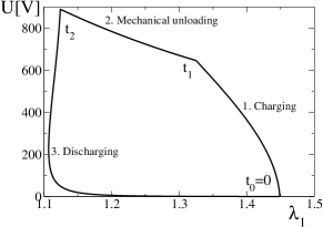
Figure 2: An example of a cycle with the default values listed in Table 1. The phase of the driving force is $\varphi=1.75929$ and the switching times are $t_{1}=1.8\,\mathrm{s}$ and $t_{2}=4.32\,\mathrm{s}$.

Now follows a presentation of results obtained for the variation of the parameters of the harvesting cycle, the electrical circuit, and the materials. Some such parameters could be varied easily in an operating wave power plant, while others would be fixed by technical and design choices.

The voltage-stretch curve for a simulation using the parameters listed in Table 1 are shown in Fig. 2. This particular example corresponds to fully optimized parameters for the DEAP material, which were found through procedures described in the sections below. The mechanical and dielectric parameters are taken from measurements performed on the DEAP soft capacitor material, and are consistent with the corresponding data sheets DanfossPolyPower . The phase of the driving is $\varphi=1.75929$, the switching times are $t_{1}=1.8\,\mathrm{s}$ and $t_{2}=4.32\,\mathrm{s}$. The efficiency in this particular example is $\eta=0.42$ while the gain is $G=0.47$. The total harvested energy is $W_{\rm R,Out}=5.5\,\mathrm{mJ}$. Compared to the mass of the material (the volume is $L_{1}^{\prime}L_{2}^{\prime}L_{3}^{\prime}=10^{-6}\,\mathrm{m^{3}}$, while the density is $1100\,\mathrm{kg\,m^{-3}}$), the specific harvested energy for one cycle becomes $5\,\mathrm{Jkg^{-1}}$. Of course, this is small compared to energy density of $1500\,\mathrm{Jkg^{-1}}$ (from Pelrine2001 ), which applies to the special case of prestretched polyacrylate glue. However, the result obtained here is more realistic; it is found by considering a full cycle, maximizing $\eta$ and with a limitation of the electrical field to a reasonable level of $20\,\mathrm{Vm^{-1}}$.

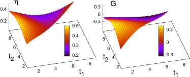
Figure 3: The harvesting efficiency $\eta$ and the gain $G$ in dependence of the switching times $t_{1}$ and $t_{2}$. The surfaces are triangular because $t_{1}<t_{2}$. The phase is fixed $\varphi=1.75929$.

III.1 Cycle parameter optimization

The harvesting cycle allows a variation of the switching times $t_{1}$, $t_{2}$ and the phase $\varphi$. Their impact on the optimal efficiency $\eta$ and gain $G$ is shown in Fig. 3 for the DEAP material (see Tab. 1); the phase is fixed in this plot to $\varphi=1.76$. As expected, efficiency and gain depend strongly on the cycle parameters. Note also that regions of maximum gain and maximum efficiency do not overlap perfectly. Hence, an optimization strategy for efficiency could result in zero energy gain and vice versa.

In the following, both efficiency and gain are optimized in dependence of the circuit and material parameters. For each parameter set, $t_{1}$, $t_{2}$ and $\varphi$ are varied to maximize the efficiency and the gain, either by a Monte Carlo method using random sampling or the simplex method Numerical-Recipes .

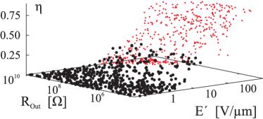
Figure 4: The efficiency in dependence of $E^{\prime}=U_{\rm In,Max}/L_{3}^{\prime}$ and $R_{\rm out}$. The values of $t_{1}$, $t_{2}$ and $\varphi$ have been optimized with help of the simplex method. Cycles violating the breakdown criteria have are plotted in red.

III.2 Electrical circuit optimization

In a power plant setting, the parameters $U_{\rm In,Max}$ and $R_{\rm Out}$ are adjustable. So is $R_{\rm In}$, though this would typically increase loss, and thus is not studied further here. Fig. 4 illustrates the result of this optimization. It was obtained by first choosing random values for $E^{\prime}=U_{\rm In,Max}/L_{3}^{\prime}$ and $R_{\rm Out}$ in the ranges shown, then optimizing the efficiency by adjusting $t_{1}$, $t_{2}$, $\varphi$ via the simplex method. If the breakdown criteria are violated, the particular data point is plotted in red. The material properties are again taken from Tab. 1. Clearly, the efficiency increases if the driving voltage increases. It is bounded by the breakdown criteria, and it is relatively unaffected by the output resistance in the investigated range. The maximum observed harvesting efficiency was about 0.42.

Figure 5: Evaluation of the effect of material properties. The upper and lower rows show optimized efficiency $\eta$ and gain $G$, respectively, in dependency of relative permittivity $\varepsilon_{r}$ and polymer conductivity $\sigma_{\rm DC}$. The graphs in the left column was for polymer modulus $Y=1.2\,\mathrm{MPa}$, in the right for $Y=5\,\mathrm{MPa}$.

III.3 Dielectric material parameter optimization

Fig. 5 shows the numerically optimized efficiency for varying polymer conductivity $\sigma_{\rm DC}$ and permittivity $\varepsilon_{\rm rel}$ for two different values of the stiffness of the polymer. The stiffness is varied by scaling of $C_{10}$, $C_{20}$, and $C_{30}$. For each individual parameter set ($\varepsilon_{r}$, $\sigma_{\rm DC}$) 1000 randomized sets of values of $U_{\rm In}$, $R_{\rm Out}$, $t_{1}$, $t_{2}$ and $\varphi$ were generated; other parameter are held fixed, cf. Table 1. Out of these data sets, the one with the highest value of $\eta$ (or $G$) not violating the limit criteria was determined and plotted (therefore, the observed $\eta$ and $G$ do not correspond to identical $U_{\rm In}$, $R_{\rm Out}$, $t_{1}$, $t_{2}$ and $\varphi$ values).

The results in Fig. 5 confirm intuition: First, $\eta$ generally decreases with $\sigma_{\rm DC}$ and increases with $\varepsilon_{r}$. As has been suspected, but not clearly demonstrated before, it is found here that the stiffer material can achieve a higher efficiency, for identical $\sigma_{\rm DC}$ and $\varepsilon_{r}$. Gain $G$ and efficiency $\eta$ behave similarly, but now the stiffer material has the lower response, because they undergo smaller strains and thus smaller relative change in the capacitance. The drop in gain appears less pronounced than the increase in efficiency, which indicates that stiffer elastomers are advantageous for energy harvesting.

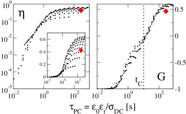
Figure 6: The efficiency $\eta$ and the gain $G$ in dependence of the Maxwell time $\tau_{\rm PC}$. The data are identical to Fig. 5 with $Y=1.2\,\mathrm{MPa}$. The inset shows a semilogarithmic plot for $\eta$. The big red diamonds show the results for the DEAP material.

Fig. 5 shows also that both $\eta$ and $G$ depend roughly on $\varepsilon_{r}\times\sigma_{\rm DC}^{-1}$. We note that this is nearly the expression for the time constant of the charge decay in the capacitor, $\tau_{\rm PC}=\varepsilon_{r}\varepsilon_{0}/\sigma_{\rm DC}$, also known as the Maxwell relaxation time. To elucidate this observation, $\eta$ and $G$ are plotted against $\tau_{\rm PC}$, see Fig. 6. All efficiency values appear to fall below a particular threshold; below $\tau_{\rm PC}=t_{C}$, the efficiency varies with $\tau_{\rm PC}$, above it is nearly constant and are distributed between $0.2$ and $0.6$.

Also gain is seen to depend directly upon $\tau_{\rm PC}$. It collapses on a straight line in the semilogarithmic plot. Interestingly, it is only positive for $\tau_{\rm PC}>t_{C}$, clearly showing that the Maxwell relaxation time must be shorter than the period of the mechanical driving. Comparing to the efficiency plot, high gain does not necessarily lead to high efficiency as was seen previously, see Fig. 3. In summary, the highest efficiencies and gains are slightly above 0.6 and encouragingly, the DEAP material shows both good efficiency and gain.

These plots clearly show the importance of the proper choice of the time scales of the loss mechanisms, and that they must be chosen in accordance with the relevant driving time scale. Furthermore, $\tau_{\rm PC}$ can be identified as the dominant material parameter for energy harvesting.

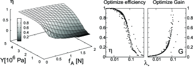
Figure 7: Left panel: the efficiency $\eta$ in dependence of the amplitude of the driving force $f_{A}$ and the stiffness $Y=8C_{10}$ of the material. Right panel: The efficiency and the gain in dependency of the $\lambda_{*}=\sigma_{\rm Amp}/Y$. The electrical material parameter are taken from 1.

III.4 Mechanical material parameter optimization

The impact of the mechanical properties of the elastomer was evaluated by varying the stress-strain properties, simply by multiplication of $C_{10}$, $C_{20}$, and $C_{30}$ with the same factor. Then, the strength of the driving force was varied and either the efficiency $\eta$ or the gain $G$ was optimized, as described above. As is clearly seen from Fig. 7 (left), the efficiency increases with higher stiffness, while it decreases for higher driving forces.

This data is efficiently analyzed when introducing a new variable, the virtual stretch $\lambda_{*}=\sigma_{\rm Amp}/Y=f_{A}/(L_{2}^{\prime}L_{3}^{\prime}/Y)$, which is a relative measure of the level of stretch during the cycle (see Fig. 7). Remarkably, this plot shows that small stretches (originating from high stiffnesses or small driving forces) result in high efficiency. The gain behaves opposite, therefore energy harvesting can only be practicable in a narrow range of $\lambda_{*}$.

IV Conclusion

In this article, energy harvesting using electro active polymers has been studied by means of numerical simulations and analytical considerations. In detail, a realistic model describing the dynamics of the polymer as a relaxation process has been presented, as well as electrical control circuits and various limiting criteria. This system is driven by a periodic force, which compares well to an energy harvesting device using ocean waves or similar (fluid) mechanical forcing, as in generators in shoes or energy producing patches. The model is generic in that all its units describe essential and necessary parts of any future realization of an energy harvesting power plant. A direct coupling between the driving force and the soft capacitor was chosen, which applies well if complicated and expensive mechanical setups have to be avoided.

The study focused on qualitative and quantitative measures (efficiency and gain) for energy harvesting and on the corresponding parameter optimization, which is important for the design of potential power plants. The study showed that optimizing charging and discharging times as well as the electrical loading parameters are crucial to obtain high efficiencies. Furthermore, it could be shown that the Maxwell time $\tau_{\rm PC}$ and the virtual stretch $\lambda_{*}$ are powerful tools in the analysis and should be tuned rationally to obtain optimal energy output. Among others, this leads to the strong conclusion that the Maxwell time must by larger than the period of the mechanical driving.

The realistic simulation of the DEAP silicone material shows a specific harvesting energy density of $5\,\mathrm{Jkg^{-1}}$ for a wave period of 10 s. Assuming a realistic raw material price for silicone of $10\,\mathrm{Euro/kg}$, this study indicates that a full return of materials investment is possible within 10 years. The investment will of course be compounded by other costs, for electronics, installations and maintenance. This time span is a very conservative estimate. It can be reduced if electrical fields larger than $20\,\mathrm{V\mu m^{-1}}$ are used, which could be possible with stiffer materials Kollosche2009 . Further improvements should be possible with a more elaborate charging and discharging scheme that exploits the full variable range within the limit criteria Graf2010 ; Jean-Mistral2010 . As such, this study shows that the wave energy harvesting technology based on soft capacitors has great potential for practical usability.

V Appendix: Mechanical model

The time dependent mechanical response of the polymer is given by Eq. (1) which describes a Kelvin-like fluid. It assumes that shear stresses are not present and that the material will always relax back to the equilibrium. $\gamma$ is strongly related to the mechanical relaxation time. In fact, the mechanical relaxation $\tau_{M}$ is given by $\tau_{M}^{-1}=\mbox{d}F(\lambda_{1})/\mbox{d}\lambda_{1}|_{\lambda_{1}^{\star}}\approx Y/2\gamma$, where $F(\lambda_{1})$ is the RHS of (2). A value $\gamma=10^{6}\,\mathrm{sPa^{-1}}$ was chosen resulting in a relaxation time of $\tau_{M}\approx 1.8\,\mathrm{s}$ if external forces and charges are absent.

To derive the final constitutive differential equation, the equations for $T_{11}$ and $T_{33}$ are considered

$$T_{11} = \sigma_{11}^{M}+\sigma_{11}^{E}-p=\frac{f_{1}}{A_{1}}-\gamma\dot{\lambda}_{1}$$

$$T_{33} = \sigma_{33}^{M}+\sigma_{33}^{E}-p=-\gamma\dot{\lambda}_{3}\,\,\text{,}$$

and the static pressure $p$ is eliminated to obtain

$$\left(\sigma_{11}^{M}-\sigma_{33}^{M}\right)+\left(\sigma_{11}^{E}-\sigma_{33}^{E}\right)=\frac{f_{1}}{A_{1}}-\gamma\left(\dot{\lambda}_{1}-\dot{\lambda}_{3}\right)\,\,\text{.}$$ (10)

The force is applied in $x$-direction. Furthermore, $T_{22}$ does not enter the game since pure-shear boundary conditions are assumed.

The term $\sigma_{11}^{M}-\sigma_{33}^{M}=\sigma_{\rm Mech}$ is the stress strain model and depends in general on the geometry of the polymer. The Yeoh model was chosen which agrees well with experimental results on the Danfoss material. It can be derived from $\sigma_{ii}=\lambda_{i}\partial W/\partial\lambda_{i}$. $W$ is the energy function which takes the form $W=C_{10}(I_{1}-3)+C_{20}(I_{1}-3)^{2}+C_{30}(I_{1}-3)^{3}$ for the Yeoh model with $I_{1}=\lambda_{1}^{2}+\lambda_{2}^{2}+\lambda_{3}^{2}$. Inserting the pure-shear assumptions and summarizing the terms for the $x$ and the $z$ directory lead finally to

$$\sigma_{\rm Mech}=2\left(\lambda_{1}^{2}-\lambda_{1}^{-2}\right)\left(C_{10}+2C_{20}\Lambda+3C_{30}\Lambda^{2}\right)$$ (11)

with $\Lambda=\lambda_{1}^{2}+\lambda_{1}^{-2}-2$. Usually the stiffness of materials is quantified by the Youngs modulus $E$, which is defined as $Y=\frac{\partial\sigma}{\partial\lambda}\big{|}_{\lambda=1}$. For the Yoeh model under pure shear conditions this results in $Y=8C_{10}$.

The second term on the LHS of (10) is the Maxwell stress Kofod2005 ; Suo2008

$$\sigma_{\rm Elec}=\sigma_{11}^{E}-\sigma_{33}^{E}=-\varepsilon_{r}\varepsilon_{0}E_{3}^{2}=-\varepsilon_{r}\varepsilon_{0}\frac{U^{2}}{L_{3}^{\prime 2}}\lambda_{1}^{2}\,\,\text{,}$$ (12)

where $E_{3}$ is the electrical field and $U$ the voltage between the electrodes.

References

- (1) Joao Cruz, editor. Ocean Wave Energy. Springer, New York, 2008.
- (2) G. Dalton and B. P. Ó Gallachóir. Building a wave energy policy focusing on innovation, manufacturing and deployment. Renew. Sust. Energ. Rev., 14(8):2339 – 2358, 2010.
- (3) Ron Pelrine, Roy D. Kornbluh, Joseph Eckerle, Philip Jeuck, Seajin Oh, Qibing Pei, and Scott Stanford. Dielectric elastomers: generator mode fundamentals and applications. In Yoseph Bar-Cohen, editor, Smart Structures and Materials 2001: Electroactive Polymer Actuators and Devices, volume 4329, pages 148–156. SPIE, 2001.
- (4) Claire Jean-Mistral, Skandar Basrour, and Jean-Jacques Chaillout. Dielectric polymer: scavenging energy from human motion. volume 6927, page 692716. SPIE, 2008.
- (5) C. Graf, M. Aust, J. Maas, and D. Schapeler. Simulation model for electro active polymer generators. In Proc. ACTUATOR, Bremen, page P73, 2010.
- (6) Paul Brochu, Huafeng Li, Xiaofan Niu, and Qibing Pei. Factors influencing the performance of dielectric elastomer energy harvesters. volume 7642, page 76422J. SPIE, 2010.
- (7) Seiki Chiba, Mikio Waki, Roy Kornbluh, and Ron Pelrine. Extending applications of dielectric elastomer artificial muscle. In Yoseph Bar-Cohen, editor, Proc. SPIE-EAPAD, volume 6524, page 652424, 2007.
- (8) Seiki Chiba, Mikio Waki, Roy Kornbluh, and Ron Pelrine. Innovative power generators for energy harvesting using electroactive polymer artificial muscles. In Yoseph Bar-Cohen, editor, Proc. SPIE-EAPAD, volume 6927, page 692715, 2008.
- (9) Ron Pelrine, Roy Kornbluh, Qibing Pei, and Jose Joseph. High-speed electrically actuated elastomers with strain greater than 100%. Science, 287:836–839, 2000.
- (10) Federico Carpi, Danilo De Rossi, Roy Kornbluh, Ronald Pelrine, and Peter Sommer-Larsen, editors. Dielectric elastomers as electromechanical transducers. Elsevier, Amsterdam, 2008.
- (11) Paul Brochu and Qibing Pei. Advances in dielectric elastomers for actuators and artificial muscles. Macromol. Rapid Comm., 31(1):10–36, 2010.
- (12) Federico Carpi, Siegfried Bauer, and Danilo De Rossi. Stretching dielectric elastomer performance. Science, 330(6012):1759–1761, 2010.
- (13) C Jean-Mistral, S Basrour, and J-J Chaillout. Comparison of electroactive polymers for energy scavenging applications. Smart Mater. and Struct., 19(8):085012, 2010.
- (14) Mohammed Benslimane, Peter Gravesen, and Peter Sommer-Larsen. Mechanical properties of dielectric elastomer actuators with smart metallic compliant electrodes. In Proc. SPIE-EAPAD, volume 4695, pages 150–157, 2002.
- (15) Danfoss PolyPower A/S. “094F0031 Film Kit Engineering Sheet 15-12-2009,” Technical Data Sheet.
- (16) Mohamed Y Benslimane, Hans-Erik Kiil, and Michael J Tryson. Dielectric electro-active polymer push actuators: performance and challenges. Polymer International, 59(3):415–421, 2010.
- (17) C. Graf, M. Aust, J. Maas, and D. Schapeler. Simulation model for electro active polymer generators. In Proc. 10th IEEE-ICSD, Potsdam, pages G1–1, 2010.
- (18) F. Carpi, G. Gallone, F. Galantini, and D. De Rossi. Silicone–poly(hexylthiophene) blends as elastomers with enhanced electromechanical transduction properties. Adv. Funct. Mater., 18(2):235–241, 2008.
- (19) Martin Molberg, Daniel Crespy, Patrick Rupper, Frank Nüesch, Jan-Anders E. Månson, Christiane Löwe, and Dorina M. Opris. High breakdown field dielectric elastomer actuators using encapsulated polyaniline as high dielectric constant filler. Adv. Funct. Mater., 20(19):3280–3291, 2010.
- (20) Giuseppe Gallone, Fabia Galantini, and Federico Carpi. Perspectives for new dielectric elastomers with improved electromechanical actuation performance: composites versus blends. Polym. Int., 59(3):400–406, 2010.
- (21) Hristiyan Stoyanov, Matthias Kollosche, Denis N. McCarthy, and Guggi Kofod. Molecular composites with enhanced energy density for electroactive polymers. J. Mater. Chem., 20:7558–7564, 2010.
- (22) Hristiyan Stoyanov, Matthias Kollosche, Sebastian Risse, Denis N. McCarthy, and Guggi Kofod. Elastic block copolymer nanocomposites with controlled interfacial interactions for artificial muscles with direct voltage control. Soft Matter, pages –, 2010.
- (23) Hal F. Brinson and L. Catherine Brinson. Polymer Engineering Science and Viscoelasticity: An Introduction. Springer, Berlin, December 2007.
- (24) Guggi Kofod and Peter Sommer-Larsen. Silicone dielectric elastomer actuators: Finite-elasticity model of actuation. Sens. Actuat. A, 122(2):273–283, aug 2005.
- (25) O. H. Yeoh. Some forms of the strain energy function for rubber. Rubber Chem. Technol., 66(5):754–771, 1993.
- (26) Zhigang Suo, Xuanhe Zhao, and William H. Greene. A nonlinear field theory of deformable dielectrics. J. Mech. Phys. Solids, 56(2):467 – 486, 2008.
- (27) L. Di Lillo, A. Schmidt, A. Bergamini, P. Ermanni, and E. Mazza. Dielectric and insulating properties of an acrylic dea material at high near-dc electric fields. volume 7976, page 79763B. SPIE, 2011.
- (28) Xuanhe Zhao and Zhigang Suo. Method to analyze electromechanical stability of dielectric elastomers. Appl. Phys. Lett., 91(6):061921, 2007.
- (29) .
- (30) Ernst Hairer and Gerhard Wanner. Solving Ordinary Differential Equations II: Stiff and Differential-Algebraic Problems. Springer, Berlin, February 2010.
- (31) William H Press, Saul A Teukolsky, William T Vetterling, and Brian P Flannery. Numerical Recipes 3rd Edition: The Art of Scientific Computing. Cambridge University Press, September 2007.
- (32) Matthias Kollosche and Guggi Kofod. Electrical failure in blends of chemically identical, soft thermoplastic elastomers with different elastic stiffness. Appl. Phys. Lett., 96(7):071904, 2010.