Edge effects in graphene nanostructures:
I. From multiple reflection expansion to density of states

Abstract

We study the influence of different edge types on the electronic density of states of graphene nanostructures. To this end we develop an exact expansion for the single particle Green’s function of ballistic graphene structures in terms of multiple reflections from the system boundary, that allows for a natural treatment of edge effects. We first apply this formalism to calculate the average density of states of graphene billiards. While the leading term in the corresponding Weyl expansion is proportional to the billiard area, we find that the contribution that usually scales with the total length of the system boundary differs significantly from what one finds in semiconductor-based, Schrödinger type billiards: The latter term vanishes for armchair and infinite mass edges and is proportional to the zigzag edge length, highlighting the prominent role of zigzag edges in graphene. We then compute analytical expressions for the density of states oscillations and energy levels within a trajectory based semiclassical approach. We derive a Dirac version of Gutzwiller’s trace formula for classically chaotic graphene billiards and further obtain semiclassical trace formulae for the density of states oscillations in regular graphene cavities. We find that edge dependent interference of pseudospins in graphene crucially affects the quantum spectrum.

I Introduction

I.1 Graphene-based nanostructures

Triggered by the experimental discovery of massless Dirac quasiparticlesNovoselov et al. (2004, 2005), graphene has become one of the most intensively studied materials of the last decade (for reviews on physical properties see Refs. Geim and Novoselov, 2007; Avouris et al., 2007; Beenakker, 2008; Castro Neto et al., 2009; Abergel et al., 2010).

Subsequently, graphene-based nanostructures have been the focus of an immense experimental activity, including graphene nanoribbonsHan et al. (2007); Li et al. (2008); Tapaszto et al. (2008); Gallagher et al. (2010), quantum dots Ponomarenko et al. (2008); Güttinger et al. (2008, 2010), Aharonov-Bohm ringsRusso2008 ; Huefner2010 and antidot arraysEroms and Weiss (2009); Bai et al. (2010), raising the issue of confining massless Dirac electrons. On the theoretical side, several studies have also focused on graphene nanostructures: Graphene nanoribbons have been studied first using a lattice modelFujita et al. (1996); Nakada et al. (1996). The wavefunctions and energy spectra of graphene nanoribbons have been derived by Brey and FertigBrey and Fertig (2006a) for armchair and zigzag type edges, and by Tworzydło and coworkersTworzydlo2006 for the case of infinite mass edges. The spectral and transport properties of Dirac electrons confined in graphene quantum dots have been investigated analyticallySilvestrov and Efetov (2007); Trauzettel et al. (2007); Recher2009 and by numerical meansBardarson2009 ; Libisch et al. (2009); Wurm et al. (2009a); Wimmer et al. (2010). Also energy spectrum and conductance of Aharonov-Bohm rings have been the focus of several publicationsRecher2007 ; Wurm2010 ; Schelter et al. (2010) as well as superlattice effects in graphene antidot latticesPedersen et al. (2008); Vanević et al. (2009) and the density of states of nanoribbon-superconductor junctionsHerrera2010 .

One upshot of these studies is the understanding that the confinement of charge carriers in graphene affects the coherent electron and hole dynamics considerably. In conventional two-dimensional electron systems (2DES) such as low-dimensional semiconductor structures, the charge carriers can be confined, e.g. by the application of top or side gate voltages, and the quasiparticle transport does not depend on the minute details of the resulting effective potential. In contrast, in graphene, electrostatic potentials do not necessarily confine charge carriers as the Dirac spectrum does not have a gapBeenakker (2008). Thus the confined electrons or holes in graphene nanostructures or flakes are expected to scatter from the very ends of the terminated graphene lattice, and the internal degrees of freedom (such as spin or pseudospin) of the quasiparticles before and after the scattering are considerably affected by the atomic level details of the edges. This mixing of internal (pseudo)spin with orbital degrees of freedom of charge carriers at the boundary leads to richer boundary conditions than for the conventional 2DESMcCann and Fal’ko (2004); Akhmerov and Beenakker (2007, 2008). These boundary conditions in turn affect the spectral and transport properties. However, experimental control and manipulation of edges at an atomistic level is far from being achieved. Thus a full theoretical description is desirable. However, the edge disorder differs from usual (weak) bulk disorder in that weak coupling perturbation theories cannot treat edges. Therefore this paper is dedicated to develop a formalism that includes the effects of edges non-perturbatively, and to subsequently apply this formalism to study edge effects on the spectral density of states of graphene nanostructures.

I.2 Scope of this work

Cutting a finite piece of graphene out of the bulk will generally lead to disordered boundaries with local properties depending on the respective orientation of an edge segment with respect to the crystallographic axes. The accurate calculation of the eigenenergies these finite graphene systems usually requires numerical quantum mechanical approaches. However, it appears difficult to systematically resolve edge phenomena from other quantum effects or to unravel generic features of graphene nanostructures using numerical simulations. Here we follow a complementary strategy: We adapt the multiple reflection expansionBalian and Bloch (1970); Adagideli and Goldbart (2002), i. e. a representation of the Green’s function in terms of the number of reflections from the system boundaries, to the case of graphene. We thus incorporate edge effects (due to armchair, zigzag and infinite mass type and combinations of such edge segments) in a direct and transparent way. We next derive a semiclassical approximation for the Green’s function, assuming the Fermi wavelength is much smaller that the typical system size $L$, i. e. $L\gg 1/k_{\scriptscriptstyle E}$. On the other hand, the Dirac equation that we use is valid for Fermi wavelengths that are large compared to the lattice constant $a\approx 2.46$ Å , i. e. if $1/k_{\scriptscriptstyle E}\gg a$. For mesoscopic systems with $L\gg a$, the semiclassical approximation can thus be well fulfilled in the linear dispersion regime, in which quasiparticle dynamics is governed by the effective Dirac equation. The resulting Green’s function then can be used to calculate the density of states (DOS) or the conductance, and their correlators.

In this work we consider the density of states. We focus on gross structures and spectral densities arising from moderate smearing of the level density and on the calculation of DOS oscillations and individual levels separately. To this end we decompose the DOS into an average part and the remaining oscillatory contribution. The average spectral density, approximated by the so-called Weyl expansion Weyl (1911); Balian and Bloch (1970); Gutzwiller (1990) valid in the semiclassical limit, is a fundamental quantity of a cavity. It incorporates various geometrical and quantum features, including edge effects. For billiards with spin-orbit interaction, the smooth part of the engery spectrum has been studied in Ref. Cserti2004, . The oscillatory part of the DOS is computed by invoking a semiclassical approximation, leading to so-called semiclassical trace formulae, i. e. sums over coherent amplitudes associated to classical periodic orbits. For graphene cavities with shapes giving rise to regular or chaotic classical dynamics we derive trace formulae analogous to those known (Berry-Tabor Berry1976/77 and Gutzwiller Gutzwiller (1990) formula, respectively) for the corresponding Schrödinger billiards, i. e. billiard systems based on the Schrödinger equation with Dirichlet boundary conditions. For two representative regular shapes, we compute the DOS oscillations and the semiclassical energy levels explicitly. The effects of both, the underlying effective Dirac equation (for graphene close to the Dirac point) and reflections at different kinds of edges, is incorporated by a pseudospin propagator associated with each orbit, multiplying the usual semiclassical amplitude. Semiclassical trace formulae involving the electron spin dynamics have been earlier considered for the massive Dirac equation by Bolte and Keppeler Bolte1999 and for bulk graphene by Carmier and Ullmo Carmier and Ullmo (2008). Related trace formulae appear also in trajectory-based treatments of electronic systems with spin-orbit interaction Pletyukhov2002 ; Chang2004 ; Zaitsev2005 ; Adagideli2010 . We note that semiclassical methods have also been used to study graphene in magnetic fieldsKormanyos2008 ; Rakyta2010 ; Carmier2010 .

Following the concepts outlined above we address edge effects on the electronic spectra of closed graphene cavities and quantum transport through open graphene systems in two consecutive papers. In the present paper we first derive the single-particle Green’s function and its semiclassical approximation for graphene cavities and calculate the density of states. In subsequent workpartII we will consider quantities based on products of single-particle Green’s functions. They include the transport quantities such as the conductance as well as the spectral two-point correlator and its dual the spectral form factor, as a tool to study spectral statistics. The semiclassical treatment of observables based on products of Green’s functions requires additional techniques which builds the conceptual basis of the second paperpartII .

The present paper is organized as follows: After introducing below the effective Hamiltonian and (matrix) boundary conditions for the different edge types, we derive in Sec. II the multiple reflection expansion (MRE) for the Green’s function of a ballistic graphene structure. With this expansion as a starting point we then compute in Sec. III the first two terms in the Weyl expansion for the smooth part of the DOS of graphene billiards, particularly focusing on contributions from the boundary. We compare our analytical theory with numerical quantum simulations for various graphene billiards with different edge structures. In Sec. IV we turn to the oscillatory part of the DOS . To this end we first obtain a general semiclassical approximation to the MRE for the graphene Green’s function in terms of sums over classical trajectories in IV.1. Subsequently we focus on the DOS oscillations in graphene billiards with regular classical dynamics in IV.2. We give semiclassical trace formulae for two exemplary geometries, namely disks and rectangles, and discuss the effects of the graphene edges. Finally we extend Gutzwiller’s trace formula for the oscillatory part of the DOS to graphene cavities with chaotic classical dynamics in IV.3. We conclude in Sec. V and gather further technical material in the appendices.

I.3 Hamiltonian and boundary conditions

Neglecting the conventional spin degree of freedom, the effective Hamiltonian that describes electron and hole dynamics in graphene close to half filling is Wallace (1947)

$$\tilde{H}=v_{\scriptscriptstyle F}\tau_{z}\otimes\sigma_{x}\,p_{x}+v_{\scriptscriptstyle F}\tau_{0}\otimes\sigma_{y}\,p_{y}\,,$$ (1)

where $v_{\scriptscriptstyle F}$ is graphene’s Fermi velocity. The $\{\sigma_{i}\}$ denote Pauli matrices in sublattice pseudospin space and Pauli matrices in valley-spin space are repesented by $\{\tau_{i}\}$, while $\sigma_{0}$ and $\tau_{0}$ are unit matrices acting on the corresponding spin space. In the following, we usually omit the latter. The Hamiltonian (1) acts on spinors $[\psi_{A},\psi_{B},\psi_{A}^{\prime},\psi_{B}^{\prime}]$ where A/B stands for the sublattice index and the primed and unprimed entries correspond to the two valleys. We find it convenient to transform Eq. (1) to the valley isotropic form Akhmerov and Beenakker (2007) using the unitary transformation

$$\mathcal{U}=\frac{1}{2}(\tau_{0}+\tau_{z})\otimes\sigma_{0}+\frac{i}{2}(\tau_{0}-\tau_{z})\sigma_{y}\,.$$ (2)

The transformed Hamiltonian is

$$H=\mathcal{U}^{\dagger}\tilde{H}\mathcal{U}=v_{\scriptscriptstyle F}\tau_{0}\otimes\boldsymbol{\sigma}\!\cdot\!\mathbf{p}$$ (3)

and acts on spinors $[\psi_{A},\psi_{B},-\psi_{B}^{\prime},\psi_{A}]$.

We consider a graphene flake in which electron and hole dynamics is confined to an area $\mathcal{V}$. The boundary condition on the spinors at a point $\boldsymbol{\alpha}$ on the boundary $\partial\mathcal{V}$ is expressed as $P_{\boldsymbol{\alpha}}\psi|_{\boldsymbol{\alpha}}=0$, where $P_{\boldsymbol{\alpha}}$ is a $4\times 4$ projection matrix McCann and Fal’ko (2004); Akhmerov and Beenakker (2007). Throughout this paper we reserve bold Greek letters for boundary points and bold Roman letters for points in the bulk of the flake. For the most common boundaries, i. e. zigzag (zz), armchair (ac) and infinite mass (im), the boundary matrices are given byAkhmerov and Beenakker (2008)

$$P_{\boldsymbol{\alpha}}=\frac{1}{2}\left(1-\boldsymbol{\nu}\!\cdot\!\boldsymbol{\tau}\otimes\boldsymbol{\eta}\!\cdot\!\boldsymbol{\sigma}\right)$$ (4)

where the vectors $\boldsymbol{\nu}$ and $\boldsymbol{\eta}$ are summarized in Tab. 1. $K=4\pi/3a$ is the distance of the Dirac points from the $\Gamma$-point of the reciprocal space, $x_{\boldsymbol{\alpha}}=\boldsymbol{\alpha}\cdot\boldsymbol{\hat{x}}$ and $\boldsymbol{\hat{t}_{\alpha}}$ is the direction of the tangent to $\partial\mathcal{V}$ at $\boldsymbol{\alpha}$. For zigzag edges the sign in $\boldsymbol{\eta}$ is determined by the sublattice of which the zigzag edge consists. For an $A$-edge the upper sign is valid and for a $B$-edge the lower sign. That means the orientation of the edge effectively determines $\boldsymbol{\eta}$. For armchair edges, the upper sign is valid when the order of the atoms within each dimer is $A$-$B$ along the direction of $\boldsymbol{\hat{t}_{\alpha}}$, and the lower sign is valid for $B$-$A$ ordering. For infinite mass edges, the sign depends only on the sign of the infinite mass. The upper sign is valid for the mass going to $+\infty$ outside of $\mathcal{V}$ and the lower for the mass going to $-\infty$.

We note that for a model that includes next nearest neighbour hopping (nnn), the boundary conditions need to be modified to include differential operations on the spinor. Nevertheless, as we shall show in App. B, it is possible to modify our formalism to account for nnn hopping approximately by keeping only nearest neighbor hoppings, but modifying the boundary conditions introducing an edge potential.

	zz	ac	im
$\boldsymbol{\nu}~{}$	$\boldsymbol{\hat{z}}$	$-\sin(2Kx_{\boldsymbol{\alpha}})\boldsymbol{\hat{x}}$	$\boldsymbol{\hat{z}}$
		$+\cos(2Kx_{\boldsymbol{\alpha}})\boldsymbol{\hat{y}}$
$\boldsymbol{\eta}~{}$	$\pm\boldsymbol{\hat{z}}$	$~{}\pm\boldsymbol{\hat{t}_{\alpha}}$	$~{}\pm\boldsymbol{\hat{t}_{\alpha}}~{}$

Table 1: The vectors $\boldsymbol{\nu}$ and $\boldsymbol{\eta}$ for zigzag (zz), armchair (ac) and infinite mass (im) type boundaries.

I.4 Single particle density of states

The single particle DOS for a closed system is defined asnote_1

$$\rho(k_{\scriptscriptstyle E})=\sum_{n}\delta\left(k_{\scriptscriptstyle E}-k_{n}\right)\,.$$ (5)

Here $n$ labels the eigenenergies $E_{n}=\hbar v_{\scriptscriptstyle F}k_{n}$, and we define $E=\hbar v_{\scriptscriptstyle F}k_{\scriptscriptstyle E}$. In our derivation below we use the relation between the DOS and the retarded Green’s function of a system,

$$\rho(k_{\scriptscriptstyle E})=-\frac{1}{\pi}\mathfrak{Im}\int\limits_{\mathcal{V}}\!d\boldsymbol{x}\,\text{Tr}\left[G(\boldsymbol{x},\boldsymbol{x})\right]\,,$$ (6)

where the Green’s function $G$ fulfills

$$(E+i\eta-H)G(\boldsymbol{x},\boldsymbol{x}^{\prime})=\hbar v_{\scriptscriptstyle F}\delta(\boldsymbol{x}-\boldsymbol{x}^{\prime})\,,$$ (7)

with the Hamiltonian $H$ acting on the first argument of $G$. For a mesoscopic graphene flake the mean level spacing $\Delta k$, which is given by the inverse area of the system, is typically of the order $10^{-4}\,1/a$ or smaller. This means that $\rho$ is in principle a rapidly oscillating function of $k_{\scriptscriptstyle E}$. However, one can decompose $\rho$ into a smooth part $\bar{\rho}$ and an oscillating part $\rho_{\text{osc}}$ in a well defined wayBrack and Bhaduri (2008); Gutzwiller (1990),

$$\rho=\bar{\rho}+\rho_{\text{osc}}\,.$$ (8)

In this work, we address both contributions to $\rho$ and focus on the particularities that arise due to the spinor character and the linear dispersion of quasiparticles in graphene. The smooth part $\bar{\rho}$ represents the density of states in the limit of strong level broadening. Technically, level broadening is achieved by adding a finite imaginary part to the Fermi energy or in other words considering a real self energy. This corresponds to an exponential damping of the Green’s function and therefore only trajectories of short length, in the limiting case of ‘zero-length’, contribute. In Sec. III we treat $\bar{\rho}$ in detail. On the other hand, $\rho_{\text{osc}}$ is connected to (periodic) orbits of finite length, and in Sec. IV we use a semiclassical approach to describe this part of the density of states.

In the following, we derive an exact expression for the Green’s function entering Eq. (6) and later also its asymptotic form in the semiclassical limit, valid for large system sizes.

II The multiple reflection expansion for graphene

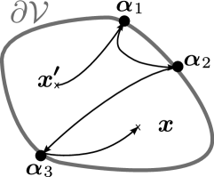
Figure 1: Schematic representation of a quantum path contributing to the Green’s function $G(\boldsymbol{x},\boldsymbol{x}^{\prime})$. The black lines with arrows stand for free propagations described by $G_{0}$, while each black disk represents a vertex of the form $i\sigma_{\boldsymbol{n_{\alpha}}}P_{\boldsymbol{\alpha}}$.

In this chapter, we derive a formula for the exact Green’s function of a graphene cavity. The Green’s function can then be used to obtain e. g. the spectral density of states or the conductance. In addition to Eq. (7), $G$ also obeys the boundary conditions $P_{\boldsymbol{\alpha}}G(\boldsymbol{\alpha},{\bf x}^{\prime})=0$ for any given point $\boldsymbol{\alpha}$ on the boundary.

We now parameterize the full Green’s function as a sum of the free retarded Green’s function $G_{0}$ of extended graphene and a boundary correction that is produced by a, yet unknown, Dirac-charge layer $\mu$:

$$G(\boldsymbol{x},\boldsymbol{x}^{\prime})=G_{0}(\boldsymbol{x},\boldsymbol{x}^{\prime})-\!\!\int\limits_{\partial\mathcal{V}}\!\!d\sigma_{\boldsymbol{\beta}}\,G_{0}(\boldsymbol{x},\boldsymbol{\beta})\,i{\sigma}_{\boldsymbol{n_{\beta}}}\,\mu({\boldsymbol{\beta},\boldsymbol{x}^{\prime}})\,.$$ (9)

Here $\sigma_{\boldsymbol{v}}\equiv\boldsymbol{\sigma}\!\cdot\!\boldsymbol{v}$ for an arbitrary vector $\boldsymbol{v}$, and $\boldsymbol{n_{\beta}}$ stands for the normal unit vector at the boundary point $\boldsymbol{\beta}$ pointing into the interior of the system. The free Green’s function is obtained by solving Eq. (7) with boundary conditions $G_{0}(\boldsymbol{x},\boldsymbol{x}^{\prime})\rightarrow 0$ as $|\boldsymbol{x}-\boldsymbol{x}^{\prime}|\rightarrow\infty$. It is given by

$$G_{0}(\boldsymbol{x},\boldsymbol{x}^{\prime}) = \hbar v_{\scriptscriptstyle F}\langle\boldsymbol{x}|(E-H)^{-1}|\boldsymbol{x^{\prime}}\rangle$$ (10)

$$= -\frac{i}{4}(k_{\scriptscriptstyle E}-i\boldsymbol{\nabla}_{\boldsymbol{x}}\!\cdot\!\boldsymbol{\sigma})H_{0}^{+}(k_{\scriptscriptstyle E}|\boldsymbol{x}-\boldsymbol{x}^{\prime}|)\,,$$

where $H_{0}^{+}$ denotes the zeroth order Hankel function of the first kind. The free Dirac Green’s function can be expressed in terms of the free Schrödinger Green’s function $g_{0}$ as

$$G_{0}(\boldsymbol{x},\boldsymbol{x}^{\prime})=(k_{\scriptscriptstyle E}-i\boldsymbol{\nabla}_{\boldsymbol{x}}\!\cdot\!\boldsymbol{\sigma})g_{0}(\boldsymbol{x},\boldsymbol{x}^{\prime})\,.$$ (11)

The Schrödinger Green’s function $g_{0}$ is a solution to

$$(k_{\scriptscriptstyle E}^{2}+i\eta-\hat{p}^{2}/\hbar^{2})g_{0}(\boldsymbol{x},\boldsymbol{x}^{\prime})=\delta(\boldsymbol{x}-\boldsymbol{x}^{\prime})\,.$$ (12)

The parametrization in Eq. (9) is singular in the limit $\boldsymbol{x}\rightarrow\boldsymbol{\alpha}$ Balian and Bloch (1970); Adagideli and Goldbart (2002):

$$\lim_{\boldsymbol{x}\rightarrow\boldsymbol{\alpha}}G(\boldsymbol{x},\boldsymbol{x}^{\prime}) = G_{0}(\boldsymbol{\alpha},\boldsymbol{x}^{\prime})-\frac{1}{2}\mu({\boldsymbol{\alpha},\boldsymbol{x}^{\prime}})$$

$$- \int\limits_{\partial\mathcal{V}}\!d\sigma_{\boldsymbol{\beta}}G_{0}(\boldsymbol{\alpha},\boldsymbol{\beta})\,i\sigma_{\boldsymbol{n_{\beta}}}\,\mu({\boldsymbol{\beta},\boldsymbol{x}^{\prime}})\,.$$

The source of this singular behavior is the logarithmic divergence of $H_{0}^{+}(\xi)$ as $\xi\rightarrow 0$. For a detailed derivation of Eq. (II) see App. A. Multiplying (II) with $P_{\boldsymbol{\alpha}}$ and invoking the boundary conditions, we obtain an inhomogeneous integral equation for the charge layer $\mu$. As a first step we assume that $P_{\boldsymbol{\alpha}}\mu=\mu$, so that we get

$$\mu({\boldsymbol{\alpha},\boldsymbol{x}^{\prime}}) = 2P_{\boldsymbol{\alpha}}G_{0}(\boldsymbol{\alpha},\boldsymbol{x}^{\prime})$$

$$-2\int\limits_{\partial\mathcal{V}}\!d\sigma_{\boldsymbol{\beta}}\,P_{\boldsymbol{\alpha}}G_{0}(\boldsymbol{\alpha},\boldsymbol{\beta})\,i\sigma_{\boldsymbol{n_{\beta}}}\,\mu({\boldsymbol{\beta},\boldsymbol{x}^{\prime}})\,.$$

Since $P_{\boldsymbol{\alpha}}^{2}=P_{\boldsymbol{\alpha}}$, the unique solution of Eq. (II), obtained by iteration, automatically fullfills $P_{\boldsymbol{\alpha}}\mu=\mu$, and thus is already a solution of the original integral equation for $\mu$. Substituting this solution into Eq. (9), we obtain the following expansion for the exact Green’s function of a graphene flake with generic edges:

$$G(\boldsymbol{x},\boldsymbol{x}^{\prime}) = G_{0}(\boldsymbol{x},\boldsymbol{x}^{\prime})+\sum_{N=1}^{\infty}G_{N}(\boldsymbol{x},\boldsymbol{x}^{\prime})\,.$$ (15)

where

$$G_{N}(\boldsymbol{x},\boldsymbol{x}^{\prime})=(-2)^{N}\int\limits_{\partial\mathcal{V}}\!d\sigma_{\boldsymbol{\alpha}_{N}}\ldots d\sigma_{\boldsymbol{\alpha}_{2}}d\sigma_{\boldsymbol{\alpha}_{1}}\times$$ (16)

$$G_{0}(\boldsymbol{x},\boldsymbol{\alpha}_{N})i\sigma_{\boldsymbol{n_{\alpha}}_{N}}P_{\boldsymbol{\alpha}_{N}}\ldots G_{0}(\boldsymbol{\alpha}_{2},\boldsymbol{\alpha}_{1})i\sigma_{\boldsymbol{n_{\alpha_{1}}}}P_{\boldsymbol{\alpha}_{1}}G_{0}(\boldsymbol{\alpha}_{1},\boldsymbol{x}^{\prime})\,.$$

Each term in this expansion can be viewed as a sequence of free propagations connected at reflections at the boundary (see Fig. 1). We thus obtain the multiple reflection expansion (MRE). In Eq. (16) every reflection is represented by a boundary dependent projection $P_{\boldsymbol{\alpha}}$ and by $\sigma_{\boldsymbol{n_{\alpha}}}$, a reflection of the pseudospin across the normal axis given by $\boldsymbol{n_{\alpha}}$. The integrals along the boundary can be interpreted as a ‘summation’ over all quantum paths leading from $\boldsymbol{x}^{\prime}$ to $\boldsymbol{x}$. In Fig. 1, we show schematically a typical term in the MRE using the example of a quantum path that includes three reflections at the boundary. To summarize at this stage, with Eqs. (15, 16) we obtained a formalism that naturally relates the edge effects to any quantity that involves single particle Green’s functions.

III The smoothed density of states of graphene billiards

III.1 Weyl expansion

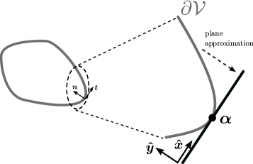
Figure 2: For the calculation of the one-reflection term in the expansion for $\bar{\rho}$, we work in the plane approximation: For a given point $\boldsymbol{\alpha}$ on the boundary $\partial\mathcal{V}$, we approximate the boundary locally by the tangent at $\boldsymbol{\alpha}$ and introduce a local coordinate system with $x$ and $y$ along the tangential and normal direction respectively.

In the following we are going to derive the leading order contributions to the smoothed density of states $\bar{\rho}$. In usual Schrödinger billiards of linear system size $L$, as they are realized e. g. in 2DES in GaAs heterostructures, $\bar{\rho}$ can be expanded in powers of $k_{E}L$ with leading order $(k_{E}L)^{1}$, a constant term $(k_{E}L)^{0}$ and higher order terms $(k_{E}L)^{-1}$, $(k_{E}L)^{-2}$ and so forth as

$$\bar{\rho}=\bar{\rho}_{0}+\bar{\rho}_{1}+\bar{\rho}_{2}+\bar{\rho}_{3}\ldots\,.$$ (17)

In the large $k_{\scriptscriptstyle E}L$ limit, $\bar{\rho}$ is dominated by the first term, which does not depend on the shape of the system but only on its total area. This theorem goes back to Hermann WeylWeyl (1911) and therefore the series is known as the Weyl expansion for the density of states. Each of the terms in Eq. (17) can be obtained from the MRE (16): $\bar{\rho}_{0}$ originates from the zero-reflection term (simply $G_{0}$) and therefore scales with the total area $A$ of the system. The term $\bar{\rho}_{1}$ is due boundary contributions, obtained within the so-called plane approximation (cf. Fig. 2), leading to a scaling with the length of the boundary. The term $\bar{\rho}_{2}$ stems from curvature and corner corrections to the plane approximation and so forth. In this work we focus on leading contributions $\bar{\rho}_{0}$ and $\bar{\rho}_{1}$. The smooth contributions are of qualitatively different origin than the oscillating part of the DOS, treated in Sec. IV. While the latter correspond to orbits for which the phases occuring in Eq. (6) are stationary, the smooth DOS is due to trajectories approaching ‘zero-length’ for which the amplitudes diverge. We find that the linear term in the Weyl expansion for graphene $\bar{\rho}_{0}$ is similar to the usual 2DES case, but the term $\bar{\rho}_{1}$ behaves strikingly different.

III.2 Bulk term

We begin with the zero-reflection term $G_{0}(\boldsymbol{x},\boldsymbol{x})$ in graphene. From Eq. (10) we can directly read off

$$\text{Tr}\left[G_{0}(\boldsymbol{x},\boldsymbol{x^{\prime}})\right]=-ik_{\scriptscriptstyle E}H_{0}^{+}(k_{\scriptscriptstyle E}|\boldsymbol{x}-\boldsymbol{x^{\prime}}|)\,.$$ (18)

Although $G_{0}$ diverges as $\boldsymbol{x^{\prime}}\rightarrow\boldsymbol{x}$,Stöckmann (1999) its imaginary part is finite. We get

$$\mathfrak{Im}\,\text{Tr}\left[G_{0}(\boldsymbol{x},\boldsymbol{x})\right]=-|k_{\scriptscriptstyle E}|\,.$$ (19)

Since there is no $\boldsymbol{x}$ dependence left, the spatial integral in Eq. (6) gives just $A=|\mathcal{V}|$, the area of the billiard, and we have

$$\bar{\rho}_{0}(k_{\scriptscriptstyle E})=\frac{A}{\pi}|k_{\scriptscriptstyle E}|\,.$$ (20)

As for Schrödinger billiards, the bulk term (20) is proportional to the total area of the system. The energy dependence of $\bar{\rho}_{0}$ is however different, since $k_{\scriptscriptstyle E}$ scales linearly with energy in graphene but has a square root dependence in the Schrödinger case.

III.3 Boundary term

III.3.1 Plane approximation

As we show below, the boundary term $\bar{\rho}_{1}$ depends on $k_{\scriptscriptstyle E}$ as well as on the boundary length of the system, in a manner distinctly different from that of Schrödinger billiards. In order to evaluate $\bar{\rho}_{1}$, we assume that the energy has a finite imaginary part $\xi$. This smoothens the DOS and makes $G_{0}$ an exponentially decaying function of the distance between $\boldsymbol{x}$ and $\boldsymbol{x^{\prime}}$. We start from Eq. (9), omit the free propagation term that led to $\bar{\rho}_{0}$, and obtain for the remaining contribution to the smooth DOS

$$\delta\bar{\rho}=\frac{1}{\pi}\mathfrak{Im}\sum_{i}\int\limits_{\partial\mathcal{V}_{i}}\!d\sigma_{\boldsymbol{\alpha}}\!\!\int\limits_{\mathcal{V}}\!d\boldsymbol{x}\,\text{Tr}\left[G_{0}(\boldsymbol{x},\boldsymbol{\alpha})i\sigma_{\boldsymbol{n_{\alpha}}}\mu_{i}(\boldsymbol{\alpha},\boldsymbol{x})\right]\,.$$ (21)

Here we replaced the boundary integration by a sum of integrations over boundary pieces $\partial\mathcal{V}_{i}$, where the boundary condition is constant for each $i$. Further $\mu_{i}(\boldsymbol{\alpha},\boldsymbol{x})$ is defined via Eq. (II) with $\boldsymbol{\alpha}\in\partial\mathcal{V}_{i}$. Since $G_{0}$ is short ranged, the dominant contribution to the boundary integral in Eq. (21) comes from configurations where $\boldsymbol{x}$ is near the boundary point $\boldsymbol{\alpha}$, and the integral in Eq. (II) is dominated by contributions where $\boldsymbol{\beta}$ is near $\boldsymbol{\boldsymbol{\alpha}}$. Thus we approximate the surface near $\boldsymbol{\alpha}$ by a plane (cf. Fig. 2). The corrections to this approximation are of order $1/k_{\scriptscriptstyle E}R$, with the local radius of curvature $R\sim L$, thus of higher order in the Weyl expansionBalian and Bloch (1970). We now take advantage of the homogeneity of the approximate surface at $\boldsymbol{\alpha}$ and use Fourier transformation along the direction of the tangent to the $\partial\mathcal{V}_{i}$ at $\boldsymbol{\boldsymbol{\alpha}}$, to get for $\delta\bar{\rho}\approx\bar{\rho}_{1}$

$$\bar{\rho}_{1}=\frac{1}{\pi}\mathfrak{Im}\!\sum_{i}|\partial\mathcal{V}_{i}|\int\limits_{0}^{\infty}\!\!dy_{i}\!\!\int\limits_{-\infty}^{\infty}\!\!\frac{dk}{2\pi}\,\text{Tr}\left[\delta G_{i}(k,y_{i})\right]\,,$$ (22)

with

$$\delta G_{i}(k,y_{i})=G_{0}(k,y_{i})i\sigma_{\boldsymbol{n_{\alpha}}}\mu_{i}(k,y_{i})\,.$$ (23)

Here $y_{i}$ is the ordinate of the local coordinate system at $\boldsymbol{\alpha}$ (see Fig. 2) and

$$\mu_{i}(k,y_{i})\! = \!2\Gamma_{i}(k)P_{\boldsymbol{\alpha}}\,G_{0}(k,-y_{i})\,,$$ (24)

$$\Gamma_{i}(k) = \left[1\!+\!2P_{\boldsymbol{\alpha}}\,G_{0}(k,0)\,i\sigma_{y}\right]^{-1}\,,$$ (25)

with the Fourier transform defined as

$$f(x,y)=\int\limits_{-\infty}^{\infty}\!\frac{dk}{2\pi}\,e^{ikx}f(k,y)\,.$$ (26)

We pushed the upper limits of the $y_{i}$-integration to infinity, which is valid when $\exp[-\mathfrak{Im}(k_{\scriptscriptstyle E})L]\ll 1$. To obtain Eq. (22), we further assumed that $\boldsymbol{\alpha}$ is away from the corners where the boundary condition changes. The corrections due to such points are of order $1/k_{\scriptscriptstyle E}L$ smaller than the boundary term.

The free Green’s function in mixed representation is given by

$$G_{0}(k,y_{i})=\frac{-e^{-a(k)|y_{i}|}}{2a(k)}\left[k\sigma_{x}+i\,\text{sgn}(y_{i})a(k)\sigma_{y}+k_{\scriptscriptstyle E}\right]$$ (27)

with

$$a(k)=\sqrt{k^{2}-k_{\scriptscriptstyle E}^{2}},\qquad\mathfrak{Re}[a(k)]>0\,.$$ (28)

Next we focus on contributions to the boundary term from various types of edges.

III.3.2 Zigzag edge

For a zigzag edge (without nnn hopping, see Tab. 1)

$$P_{\boldsymbol{\alpha}}=(1\mp\tau_{z}\otimes\sigma_{z})/2\,.$$ (29)

Then $\Gamma_{i}$ is diagonal in valley space and we can invert the valley subblocks separately giving

$$\Gamma_{i}(k)=-\frac{a(k)\pm k\tau_{z}}{k_{\scriptscriptstyle E}^{2}}\left[{a(k)-(k\sigma_{z}-ik_{\scriptscriptstyle E}\sigma_{y})(1-P_{\boldsymbol{\alpha}})}\right]\,.$$ (30)

We insert $\Gamma_{i}(k)$, Eq. (30), into Eq. (24) and take into account that $P_{\boldsymbol{\alpha}}$ is a projection matrix, i. e. $P_{\boldsymbol{\alpha}}^{2}=P_{\boldsymbol{\alpha}}$, to obtain for the Dirac-charge density

$$\mu_{i}(k,y_{i})=-2\frac{a(k)}{k_{\scriptscriptstyle E}^{2}}\left[a(k)\pm k\tau_{z}\right]P_{\boldsymbol{\alpha}}\,G_{0}(k,-y_{i})\,.$$ (31)

Substituting this expression into Eq. (23), we obtain

$$\delta G_{i}(k,y_{i})$$

$$= -2\frac{a(k)}{k_{\scriptscriptstyle E}^{2}}\left[a(k)\pm k\tau_{z}\right]G_{0}(k,y_{i})\,i\sigma_{y}\,P_{\boldsymbol{\alpha}}\,G_{0}(k,-y_{i})\,.$$

Then the trace is given by (note that $y_{i}>0$)

$$\text{Tr}\left[\delta G_{i}(k,y_{i})\right]=-\frac{2k^{2}}{a(k)k_{\scriptscriptstyle E}}e^{-2a(k)y_{i}}\,.$$ (33)

Evaluating the $y_{i}$-integral we get (note that the real part of $a(k)$ is positive)

$$\mathfrak{Im}\int\limits_{0}^{\infty}\!\!dy_{i}\!\int\frac{dk}{2\pi}\,\text{Tr}\left[\delta G_{i}(k,y_{i})\right]=k_{\text{max}}\delta_{\xi}(k_{\scriptscriptstyle E})\,,$$ (34)

where

$$\delta_{\xi}(k_{\scriptscriptstyle E})=\frac{1}{\pi}\frac{\xi}{\xi^{2}+k_{\scriptscriptstyle E}^{2}}\,,$$ (35)

and we have introduced a cut-off momentum $k_{\text{max}}\sim 1/a$. Such a cut-off is justified, since in real graphene the available $k$-space is not infinite owing to the lattice structure. We cannot calculate the precise numerical value for $k_{\text{max}}$ within our effective model. Using tight-binding calculations we estimate $k_{\text{max}}=\pi/3a$ Wimmer (2008). The result (34) means that without nnn hopping, zigzag edges lead to a DOS contribution that is strongly peaked at zero energy. The origin of this contribution is indeed the existence of zigzag edge states at zero energyFujita et al. (1996); Nakada et al. (1996); Wimmer et al. (2010); Kobayashi et al. (2005); Niimi et al. (2006). To understand this connection we consider the prefactors in Eq. (31) and Eq. (III.3.2) in the limit of $k_{\scriptscriptstyle E}\rightarrow 0$; then we have

$$\frac{a(k)}{k_{\scriptscriptstyle E}^{2}}\left[a(k)\pm k\tau_{z}\right]\approx\frac{k^{2}}{k_{\scriptscriptstyle E}^{2}}[1\pm\text{sgn}{(k)}\,\tau_{z}]\,.$$ (36)

For the upper sign, this expression is divergent in one valley for negative $k$ ($\tau=+1$) and in the other valley for positive $k$ ($\tau=-1$) as $k_{\scriptscriptstyle E}$ approaches zero. For the lower sign it is just vice versa. Thus we identify the zero-energy states that are localized at the zigzag graphene edge. In a single valley this causes a strong asymmetry in the spectrum and breaks the (effective) time reversal symmetry. Below we show that the zigzag edge states are the only contribution to the DOS that scales with the boundary length of the graphene flake. Armchair and infinite mass type edges do not contribute to the surface term. However for the zigzag edge states, the effect of nnn hopping is significantWimmer (2008); Sasaki et al. (2009); Wimmer et al. (2010). For a more realistic description of the their effects on the DOS, it is therefore necessary to consider nnn hopping for the boundary term at zigzag edges. In App. B we show that the boundary condition for zigzag edges is effectively modified due to nnn hopping resulting in a boundary matrix

$$P_{\boldsymbol{\alpha}}=\frac{1}{2}\left(1\mp\tau_{z}\otimes\sigma_{z}-it^{\prime}\sigma_{y}\pm t^{\prime}\tau_{z}\otimes\sigma_{x}\right)\,.$$ (37)

Here $t^{\prime}\ll 1$ is the ratio of the nnn hopping integral and the nearest neighbor hopping integral in the tight-binding formalism. The effect of this boundary condition is to modify Eq. (31) to

$$\mu(k,y^{\prime})=2a(k)\frac{a(k)-t^{\prime}k_{\scriptscriptstyle E}\pm k\tau_{z}}{[a(k)-t^{\prime}k_{\scriptscriptstyle E}]^{2}-k^{2}}P_{\boldsymbol{\alpha}}\,G_{0}(k,-y^{\prime})\,.$$

Note that the Eqs. (37, III.3.2) turn into the expressions (29, 31) for $t^{\prime}=0$. Following the same line of calculation we find

$$\text{Tr}\left[\delta G_{i}(k,y_{i})\right]=\frac{2k^{2}}{a(k)}\frac{t^{\prime 2}-1}{(1-t^{\prime 2})k_{\scriptscriptstyle E}+2t^{\prime}a(k)}e^{-2a(k)y_{i}}\!\!\!$$ (39)

and the corresponding contribution to the DOS is to linear order in $t^{\prime}$

$$\mathfrak{Im}\!\!\int\limits_{0}^{\infty}\!\!dy_{i}\!\int\limits_{-\infty}^{\infty}\frac{dk}{2\pi}\,\text{Tr}\left[\delta G_{i}(k,y_{i})\right]\approx\frac{1-\Theta_{\xi}(k_{\scriptscriptstyle E})}{2t^{\prime}}\,.$$ (40)

Here

$$\Theta_{\xi}(k_{\scriptscriptstyle E})=\frac{1}{\pi}\arctan(k_{\scriptscriptstyle E}/\xi)+\frac{1}{2}$$ (41)

is a smooth approximation to the Heaviside step function.

According to Eq. (40), the $k_{\scriptscriptstyle E}$-dependence of the zigzag contribution to the DOS is qualitatively altered by the inclusion of nnn hopping. It is strongly asymmetric due to the broken electron-hole symmetrynote_2 . Also the peak at zero $k_{\scriptscriptstyle E}=0$ has disappeared, because the edge states are not degenerate anymore but exhibit a linear dispersion $k_{\scriptscriptstyle E}^{\text{edge}}=k/2t^{\prime}$ as derived in App. B. Note that in tight-binding, there is still a van Hove singularity in the DOS, but it is at a distance to the $K/K^{\prime}$ points and therefore not captured by the effective theory.

III.3.3 Armchair edge

We now proceed with armchair type edges. According to Tab. 1, the boundary projection matrix is given by

$$P_{\boldsymbol{\alpha}}=\frac{1}{2}\left(1-\sigma_{x}\otimes\tau_{y}\right)\,.$$ (42)

Then we obtain

$$\Gamma_{i}(k)=1+\frac{i}{a(k)}(k_{\scriptscriptstyle E}\sigma_{y}+ik\sigma_{z})(1-P_{\boldsymbol{\alpha}})$$ (43)

and the surface Dirac-charge density reads

$$\mu_{i}(k,y_{i})=2P_{\boldsymbol{\alpha}}\,G_{0}(k,-y_{i})\,,$$ (44)

leading to [cf. Eq. (23)]

$$\delta G_{i}(k,y_{i}) = 2G_{0}(k,y_{i})\,i\sigma_{y}\,P_{\boldsymbol{\alpha}}\,G_{0}(k,-y_{i})$$ (45)

$$= -G_{0}(k,y_{i})\sigma_{z}G_{0}(k,-y_{i})\otimes\tau_{y}\,.$$

Surprisingly, since $\tau_{y}$ is off-diagonal, the trace of $\delta G_{i}$ is zero and the boundary contribution to $\bar{\rho}$ in the armchair case vanishes.

III.3.4 Infinite mass edge

The calculation for the infinite mass edge is similar and for the surface Dirac-charge density we find as for the armchair case

$$\mu_{i}(k,y_{i})=2P_{\boldsymbol{\alpha}}\,G_{0}(k,-y_{i})\,,$$ (46)

which leads to

$$\delta G_{i}(k,y_{i})=\pm G_{0}(k,y_{i})\sigma_{z}G_{0}(k,-y_{i})\otimes\tau_{z}\,.$$ (47)

Similar as for the armchair edge, this expression is traceless because $\text{Tr}\,(\tau_{z})=0$. However, we point out that even within individual valleys the boundary contribution to the DOS vanishes. This follows from the fact that

$$\int\limits_{0}^{\infty}\!dy_{i}\,\text{Tr}\left[G_{0}(k,y_{i})\sigma_{z}G_{0}(k,-y_{i})\right]\sim\frac{k}{a^{2}(k)}$$ (48)

is an odd function of $k$ and thus the corresponding integral vanishes. This last fact has been already noticed by Berry and MondragonBerry and Mondragon (1987) for massless neutrinos in relativistic billiards with infinite mass walls.

III.4 Comparison with numerical results for various graphene billiards

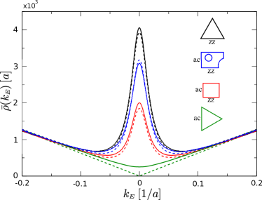
Figure 3: (color online). Smooth part of the density of states for several graphene billiards with approximately the same area $A\approx(140\,a)^{2}$, calculated numerically using a tight-binding code with only nearest neighbor coupling (solid lines). The numerical curves are obtained by first calculating exact eigenenergies and successive smoothing by replacing each energy level by a Lorentzian with a half width at half maximum of $0.015\,t$. The dashed lines are the predictions of our theory, Eq. (49). From top to bottom: black: $|\partial\mathcal{V}_{zz}|/|\partial\mathcal{V}|=1$ (zigzag triangle), blue: $|\partial\mathcal{V}_{zz}|/|\partial\mathcal{V}|\approx 1/1.6$ (Sinai shape), red: $|\partial\mathcal{V}_{zz}|/|\partial\mathcal{V}|\approx 1/1.9$ (rectangle), green: $|\partial\mathcal{V}_{zz}|/|\partial\mathcal{V}|=0$ (armchair triangle).

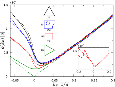
Figure 4: (color online). Smooth part of the density of states for the same systems as in Fig. 3 but with a relative next-nearest neighbor hopping strength $t^{\prime}=0.1$. Solid lines show the numerical tight-binding results and dashed lines the predictions from Eq. (50). For the smoothing we used Lorentzians with a half width at half maximum of $0.01\,t$. We used the same color coding as for Fig. 3. Inset: The tight-binding model exhibits a van Hove singularity at $k_{\scriptscriptstyle E}=-0.1\,t/\hbar v_{\scriptscriptstyle F}\approx-0.115\,1/a$. As a result the smoothed DOS shows a peak at the corresponding position (solid).

In summary, our result for the smooth DOS of a generic graphene billiard, neglecting the effect of next-nearest neighbors is

$$\bar{\rho}(k_{\scriptscriptstyle E})\approx\frac{A}{\pi}|k_{\scriptscriptstyle E}|+|\partial\mathcal{V}_{zz}|\frac{k_{\text{max}}}{\pi}\delta_{\xi}(k_{\scriptscriptstyle E})\,,$$ (49)

with $|\partial\mathcal{V}_{zz}|$ being the total length of zigzag edges in the billiard.

In Fig. 3 we compare our analytical result (49) with results from numerical simulations for the graphene billiards shown as insets. For the numerical calculations we obtain the average DOS by computing eigenvalues of a corresponding tight-binding HamiltonianWimmer and Richter (2009); Wimmer et al. (2010) and subsequent smoothing. All the billiards are chosen to have approximately the same area. This is reflected in the common slope of $\bar{\rho}$ for larger $k_{\scriptscriptstyle E}$, confirming the leading order term in the Weyl series. The different shapes and orientations give rise to different fractions of the zigzag boundary $|\partial\mathcal{V}_{zz}|/|\partial\mathcal{V}|$. While the boundaries of the equilateral triangles consist completely of either zigzag (black) or armchair (green) edges, both edge types are present in the rectangle (red) and in the non-integrable (modified) Sinai billiard (blue). We find very good agreement with our analytic prediction. We note that the dashed lines for the triangles and the rectangle do not involve any fitting, rather we have used the estimation $k_{\text{max}}=\pi/3a$ from tight-binding theory. For the Sinai billiard our theory allows to determine the total effective zigzag length $|\partial\mathcal{V}_{zz}|=516\,a$.

On the other hand, with nnn hopping we get from Eq. (40)

$$\bar{\rho}(k_{\scriptscriptstyle E})\approx\frac{A}{\pi}|k_{\scriptscriptstyle E}|+|\partial\mathcal{V}_{zz}|\frac{1-\Theta_{\xi}(k_{\scriptscriptstyle E})}{2\pi t^{\prime}}\,.$$ (50)

In Fig. 4 we compare again this analytical result (dashed) with corresponding tight-binding calculations (solid). Also here we find good agreement with our analytic predicition for the surface term. Further towards the hole regime, i. e. to more negative energies, the tight-binding model has a van Hove singularity due to the edge state band edge at $k_{\scriptscriptstyle E}=-0.1\,t/\hbar v_{\scriptscriptstyle F}\approx-0.115\,1/a$, as depicted in the inset of Fig. 4 (solid line). This peak is missing in our calculation, since in the effective Dirac theory the edge state dispersion is constantly linear for finite $t^{\prime}$ (cf. App. B). Note that also here, no additional fitting is involved (for the Sinai billiard we use $|\partial\mathcal{V}_{zz}|=516\,a$ obtained from the fit in Fig. 3).

From our discussion in this section it becomes clear that in principle the structure of a graphene flake’s boundary, i. e. the ratio between zigzag and armchair type edges, can be estimated from the behavior of the smoothed density of states at low energies. Hereby the formula (49) predicts the spectral weight of the edge states $\int_{-\infty}^{\infty}dk_{\scriptscriptstyle E}\,\bar{\rho}_{1}(k_{\scriptscriptstyle E})=|\partial\mathcal{V}_{zz}|/3a$, which is model independent, since the number of edge states is conserved. Note that Libisch et al. have numerically investigatedLibisch et al. (2009) the averaged DOS of graphene billiards and found a $\bar{\rho}(k_{\scriptscriptstyle E})$ profile similar to that in Fig. 3. Related studies on edge states in graphene quantum dots have been performed in Ref. Wimmer et al., 2010.

IV Density of states oscillations

IV.1 The multiple reflection expansion in the semiclassical limit

So far we have focused on the smooth part of the density of states. In this section we study the oscillating part $\rho_{\text{osc}}$. Our main result is an extension of Gutzwiller’s trace formulaGutzwiller (1990) to graphene systems with chaotic and regular classcial dynamics. We derive the trace formulae by evaluating Eq. (6) asymptotically in the semiclassical limit $k_{\scriptscriptstyle E}L\gg 1$. In other words we evaluate the boundary integrals in the MRE (16) using the method of stationary phase. In the limit $k_{\scriptscriptstyle E}L\gg 1$, the Hankel functions become rapidly oscillating exponential functions of the boundary points. All other terms in $G_{N}$ vary slowly along $\partial\mathcal{V}$. Thus we evaluate them at the critical boundary points where the total phase of the exponentials is stationary. There is another leading-order contribution to the boundary integrals that is of different origin, namely when the set of boundary points $\underline{\boldsymbol{\alpha}}=(\boldsymbol{\alpha}_{N},\ldots,\boldsymbol{\alpha}_{1})$ leads to a singularity in the prefactors Balian and Bloch (1972); Adagideli and Goldbart (2002). Due to the divergence of $G_{0}(\boldsymbol{\alpha},\boldsymbol{\beta})$ as $|\boldsymbol{\alpha}-\boldsymbol{\beta}|\rightarrow 0$, quantum paths involving reflections at closely lying boundary points can give rise to such singularities. We show below that short range critical points occur only at zigzag edges. We treat these short range singularities at zigzag edges by resumming the MRE leading to a renormalized reflection operator.

IV.1.1 Resummation of short range processes

The general method is outlined in Ref. Adagideli and Goldbart, 2002. Here we apply it to graphene. First we isolate the short range singularities: We define the action of an operator $\hat{\mathcal{I}}$ on a function $f$

$$\hat{\mathcal{I}}f(\boldsymbol{\alpha}):=\int\limits_{\partial V}\!d\sigma_{\boldsymbol{\beta}}\,{\mathcal{I}}(\boldsymbol{\alpha},\boldsymbol{\beta})f(\boldsymbol{\beta})\,.$$ (51)

In our case

$${\mathcal{I}}(\boldsymbol{\alpha},\boldsymbol{\beta})=2P_{\boldsymbol{\alpha}}G_{0}(\boldsymbol{\alpha},\boldsymbol{\beta})\,i\sigma_{\boldsymbol{n_{\beta}}}\,.$$ (52)

We now recast Eq. (II) as

$$\mu({\boldsymbol{\alpha},\boldsymbol{x}^{\prime}})=2P_{\boldsymbol{\alpha}}G_{0}(\boldsymbol{\alpha},\boldsymbol{x}^{\prime})-\hat{\mathcal{I}}\mu({\boldsymbol{\alpha},\boldsymbol{x}^{\prime}})\,.$$ (53)

Furthermore we decompose ${\mathcal{I}}$ into a short range part ${\mathcal{I}}_{\text{s}}$ and a long range part ${\mathcal{I}}_{\text{l}}$:

$$\begin{split}&{\mathcal{I}}_{\text{s}}(\boldsymbol{\alpha},\boldsymbol{\beta})={\mathcal{I}}(\boldsymbol{\alpha},\boldsymbol{\beta})\left[1-w(\boldsymbol{\alpha}-\boldsymbol{\beta})\right]\,,\\ &{\mathcal{I}}_{\text{l}}(\boldsymbol{\alpha},\boldsymbol{\beta})={\mathcal{I}}(\boldsymbol{\alpha},\boldsymbol{\beta})w(\boldsymbol{\alpha}-\boldsymbol{\beta})\,.\end{split}$$ (54)

Here $w(\boldsymbol{\alpha}-\boldsymbol{\beta})$ is a smooth function, that is zero whenever $\boldsymbol{\alpha}$ is close to $\boldsymbol{\beta}$ and goes to one otherwise, so that integrating over $\boldsymbol{\beta}$ isolates the critical point $\boldsymbol{\beta}=\boldsymbol{\alpha}$. This separation is however a formal one in that the specific form of $w$ does not change the final result (see Ref. Bleistein1975, for details). Then Eq. (53) leads to

$$(1+\hat{\mathcal{I}}_{\text{s}})\,\mu({\boldsymbol{\alpha},\boldsymbol{x}^{\prime}})=2P_{\boldsymbol{\alpha}}G_{0}(\boldsymbol{\alpha},\boldsymbol{x}^{\prime})-\hat{\mathcal{I}}_{\text{l}}\,\mu({\boldsymbol{\alpha},\boldsymbol{x}^{\prime}})$$ (55)

or with $\hat{\Gamma}=(\hat{1}+\hat{\mathcal{I}}_{\text{s}})^{-1}$

$$\mu({\boldsymbol{\alpha},\boldsymbol{x}^{\prime}})=2\hat{\Gamma}P_{\boldsymbol{\alpha}}G_{0}(\boldsymbol{\alpha},\boldsymbol{x}^{\prime})-\hat{\Gamma}\,\hat{\mathcal{I}}_{\text{l}}\,\mu({\boldsymbol{\alpha},\boldsymbol{x}^{\prime}})\,.$$ (56)

Now the renormalized Kernel $\hat{\mathcal{I}}_{\text{l}}$ is free of short range singularities. Alternatively, in integral representation

$$\mu({\boldsymbol{\alpha},\boldsymbol{x}^{\prime}}) = 2\int\limits_{\partial V}d\sigma_{\boldsymbol{\beta}}\,\Gamma({\boldsymbol{\alpha},\boldsymbol{\beta}})P_{\boldsymbol{\beta}}G_{0}(\boldsymbol{\beta},\boldsymbol{x^{\prime}})$$

$$-\int\limits_{\partial V}d\sigma_{\boldsymbol{\beta}}\,\int\limits_{\partial V}d\sigma_{\boldsymbol{\beta}^{\prime}}\,\Gamma({\boldsymbol{\alpha},\boldsymbol{\beta}}){\mathcal{I}}_{\text{l}}({\boldsymbol{\beta},\boldsymbol{\beta}^{\prime}})\,\mu({\boldsymbol{\beta}^{\prime},\boldsymbol{x}^{\prime}})\,.$$

We note that the relevant structure of both terms in this expression is the same, since $\mathcal{I}_{\text{l}}$ contains the isolating function $w$ and thus $\boldsymbol{\beta}^{\prime}$ can be considered to lie far away from $\boldsymbol{\beta}$ just as $\boldsymbol{x}^{\prime}$ in the first term. In this way we have formally collected all the short range contributions in $\Gamma$ and we are left with calculating

$$2\int\limits_{\partial V}\!d\sigma_{\boldsymbol{\beta}}\,\Gamma({\boldsymbol{\alpha},\boldsymbol{\beta}})P_{\boldsymbol{\beta}}G_{0}(\boldsymbol{\beta},\boldsymbol{x^{\prime}})\,.$$ (58)

We evaluate Eq. (58) again in the plane approximation and replace the boundary in the vicinity of $\boldsymbol{\alpha}$ by a straight line in the direction of the tangent at $\boldsymbol{\alpha}$. In our local coordinate system with $x$ and $y$ denoting coordinates in the tangential and normal directions, we approximate a point $\boldsymbol{\beta}$ close to $\boldsymbol{\alpha}$ by $\boldsymbol{\beta}=(x_{\boldsymbol{\beta}},y_{\boldsymbol{\beta}})\approx(\beta,0)$, and write $\boldsymbol{x^{\prime}}=(x^{\prime},y^{\prime})$ for a point $\boldsymbol{x^{\prime}}$ far away from $\boldsymbol{\alpha}$ (cf. Fig. 5). Then the system is locally homogeneous along the straight boundary and we have

$$\Gamma({\boldsymbol{\alpha},\boldsymbol{\beta}}) = \Gamma(\alpha-\beta)\,,$$ (59)

$$G_{0}(\boldsymbol{\beta},\boldsymbol{x^{\prime}}) = G_{0}(\beta-x^{\prime},-y^{\prime})\,.$$ (60)

In order to partial Fourier transform the expression (58), we use the convolution theorem to obtain ($P_{\boldsymbol{\alpha}}=P_{\boldsymbol{\beta}}$ is constant along the straight boundary)

$$\int\limits_{-\infty}^{\infty}\!d\beta\, \Gamma({{\alpha}-{\beta}})P_{\boldsymbol{\alpha}}G_{0}({\beta}-{x}^{\prime},-y^{\prime})$$ (61)

$$= \int\limits_{-\infty}^{\infty}\!dk\,e^{ik({\alpha}-{x^{\prime}})}\Gamma(k)P_{\boldsymbol{\alpha}}G_{0}(k,-y^{\prime})\,.$$

In fact we have calculated $\Gamma(k)$ already earlier, cf. Eq. (30) and Eq. (43), leading to

$$\Gamma(k)P_{\boldsymbol{\alpha}}=R_{\boldsymbol{\alpha}}(k)P_{\boldsymbol{\alpha}}$$ (62)

with the renormalizing factor

$$R_{\boldsymbol{\alpha}}(k)=\left\{\begin{array}[]{cl}-\frac{a(k)}{k_{\scriptscriptstyle E}^{2}}\left[a(k)\pm k\tau_{z}\right]&\text{for~{}zz~{}edges}\,,\\ 1&\text{for~{}ac~{}and~{}im~{}edges}\,.\end{array}\right.$$ (63)

We now define the renormalized free Green’s function through its Fourier transform as

$$\tilde{G}_{0}(\boldsymbol{\alpha},\boldsymbol{x^{\prime}}) = \int\limits_{-\infty}^{\infty}\frac{dk}{2\pi}\,e^{ik({\alpha}-{x^{\prime}})}R_{\boldsymbol{\alpha}}(k)G_{0}(k,-y^{\prime})\,.$$ (64)

Finally we cast Eq. (58) for the charge layer $\mu$ in position space into the form

$$\mu({\boldsymbol{\alpha},\boldsymbol{x}^{\prime}}) = 2P_{\boldsymbol{\alpha}}\tilde{G}_{0}(\boldsymbol{\alpha},\boldsymbol{x}^{\prime})$$

$$- 2\int\limits_{\partial\mathcal{V}}\!d\sigma_{\boldsymbol{\beta}}\,P_{\boldsymbol{\alpha}}\tilde{G}_{0}(\boldsymbol{\alpha},\boldsymbol{\beta})w(\boldsymbol{\alpha}-\boldsymbol{\beta})\,i\sigma_{\boldsymbol{n_{\beta}}}\,\mu({\boldsymbol{\beta},\boldsymbol{x}^{\prime}}).$$

The virtue of this equation is that it is free of short range singularities.

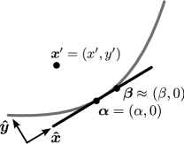
Figure 5: Notation in the local coordinate system spanned by the tangent and the normal to the boundary at $\boldsymbol{\alpha}$. Corrections to the approximation $\boldsymbol{\beta}\approx(\beta,0)$ are of subleading order in $k_{\scriptscriptstyle E}L$, cf. III.3.1.

IV.1.2 Renormalized Green’s function in the semiclassical limit

With the definition

$$\theta(k)=\arctan\left(\frac{k}{\sqrt{k_{\scriptscriptstyle E}^{2}-k^{2}}}\right)$$ (66)

we obtain from Eq. (63)

$$R_{\boldsymbol{\alpha}}(k)=\left\{\begin{array}[]{cl}\cos[\theta(k)]\,e^{\pm i\theta(k)\tau_{z}}&\text{for~{}zz~{}edges}\,,\\ 1&\text{for~{}ac~{}and~{}im~{}edges}\,.\end{array}\right.$$ (67)

We compute $\tilde{G}_{0}(\boldsymbol{\alpha},\boldsymbol{x^{\prime}})$ in Eq. (IV.1.1) by performing the Fourier integral Eq. (64) [with $R_{\boldsymbol{\alpha}}$ from Eq. (67)] within stationary phase approximation in the limit $k_{\scriptscriptstyle E}L\rightarrow\infty$. We obtain the stationary phase point $k_{0}$ from

$$\frac{d}{dk}\left[k(\alpha-x^{\prime})-\sqrt{k_{\scriptscriptstyle E}^{2}-k^{2}}\,|y^{\prime}|\right]_{k_{0}}=0$$ (68)

yielding, in view of Eq. (66),

$$\tan[\theta(k_{0})]=\frac{\alpha-x^{\prime}}{|y^{\prime}|}\,.$$ (69)

The stationary phase point $k_{0}$ is such that the angle $\theta(k_{0})$ is equal to the angle that the vector $\boldsymbol{x^{\prime}}-\boldsymbol{\alpha}$ includes with the normal at $\boldsymbol{\alpha}$, i. e. the classical angle of incidence. The stationary phase integration yields

$$\tilde{G}_{0}(\boldsymbol{\alpha},\boldsymbol{x^{\prime}})\approx R_{\boldsymbol{\alpha}}(k_{0})G_{0}^{\text{sc}}(\boldsymbol{\alpha},\boldsymbol{x^{\prime}})\,.$$ (70)

Here $G_{0}^{\text{sc}}$ is the free Green’s function in the semiclassical limit

$$G_{0}^{\text{sc}}(\boldsymbol{\alpha},\boldsymbol{\beta})=-\frac{i}{4}\sqrt{\frac{2k_{\scriptscriptstyle E}}{\pi|\boldsymbol{\alpha}-\boldsymbol{\beta}|}}e^{ik_{\scriptscriptstyle E}|\boldsymbol{\alpha}-\boldsymbol{\beta}|-i\pi/4}\left(1+\sigma_{\boldsymbol{\alpha},\boldsymbol{\beta}}\right)$$ (71)

where we use the short notation $\sigma_{\boldsymbol{\alpha},\boldsymbol{\beta}}=\boldsymbol{\sigma}\cdot(\boldsymbol{\alpha}-\boldsymbol{\beta})/|\boldsymbol{\alpha}-\boldsymbol{\beta}|$ in Eq. (71). We note that expression (71) is closely related to the semiclassical Green’s function for the free Schrödinger equation $g_{0}^{\text{sc}}$, namely

$$G_{0}^{\text{sc}}(\boldsymbol{\alpha},\boldsymbol{\beta})=k_{\scriptscriptstyle E}g_{0}^{\text{sc}}(\boldsymbol{\alpha},\boldsymbol{\beta})\left(1+\sigma_{\boldsymbol{\alpha},\boldsymbol{\beta}}\right)\,.$$ (72)

The matrix term reflects the chirality of the charge carriers in graphene: the sublattice pseudospin is tied to the propagation direction and the projection $\left(1+\sigma_{\boldsymbol{\alpha},\boldsymbol{\beta}}\right)$ takes care of this. Eq. (70) together with Eq. (IV.1.1) completes our discussion of the short range divergencies and allows us to proceed with the long range contributions to the Green’s function in the semiclassical limit.

IV.1.3 Semiclassical Green’s function for graphene cavities

In this section we evaluate the boundary integrals in the renormalized MRE in stationary phase approximation. We consider the $N$-reflection term [cf. Eq. (16)] of the renormalized MRE,

$$G_{N}(\boldsymbol{x},\boldsymbol{x^{\prime}}) \approx (-2)^{N}\prod_{i=1}^{N}\int\limits_{\partial\mathcal{V}}\!d\sigma_{\boldsymbol{\alpha}_{i}}\tilde{K}_{N}(\underline{\boldsymbol{\alpha}})\,k_{\scriptscriptstyle E}g_{0}^{\text{sc}}(\boldsymbol{x},\boldsymbol{\alpha}_{N})$$ (73)

$$\ldots ik_{\scriptscriptstyle E}g_{0}^{\text{sc}}(\boldsymbol{\alpha}_{2},\boldsymbol{\alpha}_{1})\,ik_{\scriptscriptstyle E}g_{0}^{\text{sc}}(\boldsymbol{\alpha}_{1},\boldsymbol{x^{\prime}})\,,$$

with $\underline{\boldsymbol{\alpha}}=(\boldsymbol{\alpha}_{1},..\boldsymbol{\alpha}_{i},..\boldsymbol{\alpha}_{N})$. In Eq. (73) we introduced the pseudospin propagator $\tilde{K}_{N}(\underline{\boldsymbol{\alpha}})$ that contains the graphene specific physics:

$$\tilde{K}_{N}(\underline{\boldsymbol{\alpha}}) = \left(1+\sigma_{\boldsymbol{x},\boldsymbol{\alpha}_{N}}\right)\prod_{i=1}^{N-1}\sigma_{\boldsymbol{n}_{\boldsymbol{\alpha}_{i}}}{R}_{\boldsymbol{\alpha}_{i}}P_{\boldsymbol{\alpha}_{i}}\left(1+\sigma_{\boldsymbol{\alpha}_{i+1},\boldsymbol{\alpha}_{i}}\right)$$ (74)

$$\times\sigma_{\boldsymbol{n}_{\boldsymbol{\alpha}_{1}}}P_{\boldsymbol{\alpha}_{1}}\left(1+\sigma_{\boldsymbol{\alpha}_{1},\boldsymbol{x^{\prime}}}\right)W(\underline{\boldsymbol{\alpha}})$$

with the separation function

$$W(\underline{\boldsymbol{\alpha}})=\prod_{i=1}^{N-1}w(\boldsymbol{\alpha}_{i+1}-\boldsymbol{\alpha}_{i})\,.$$ (75)

Note that the renormalization matrices ${R}_{\boldsymbol{\alpha}_{i}}$ account for possible short range singularities.

Comparing Eq. (73) with the MRE for the Helmoltz equation with Dirichlet boundary conditions Balian and Bloch (1970) shows that the scalar parts are very similar. The difference is that instead of factors $ik_{\scriptscriptstyle E}g_{0}^{\text{sc}}(\boldsymbol{\alpha}_{i+1},\boldsymbol{\alpha}_{i})$, the MRE in Ref. Balian and Bloch, 1970 has normal derivatives acting on the first argument $\boldsymbol{\alpha}_{i+1}$. In the semiclassical limit this leads to additional factors $ik_{\scriptscriptstyle E}\cos(\theta_{i+1})$, where $\theta_{i+1}$ denotes the angle between the vector $\boldsymbol{\alpha}_{i+1}-\boldsymbol{\alpha}_{i}$ and the normal vector to the boundary at $\boldsymbol{\alpha}_{i+1}$. We need not carry out the boundary integrals explicitly, but can immediately deduce

$$G^{\text{sc}}_{N}(\boldsymbol{x},\boldsymbol{x^{\prime}})=k_{\scriptscriptstyle E}{K}_{N}\,g_{N}^{\text{sc}}(\boldsymbol{x},\boldsymbol{x^{\prime}})\,,$$ (76)

where

$$K_{N}=\frac{\tilde{K}_{N}(\underline{\boldsymbol{\alpha}})}{\prod_{i=1}^{N}\cos(\theta_{i})}$$ (77)

contains the pseudospin propagator as defined in Eq. (74), but $\underline{\boldsymbol{\alpha}}$ is now the vector of the classical reflection points. The $g_{N}^{\text{sc}}(\boldsymbol{x},\boldsymbol{x^{\prime}})$ are well known, see e.g. Refs. Gutzwiller, 1990 and Baranger et al., 1993. The stationary phase condition selects all sets of $N$ stationary boundary points minimizing the phase aquired, and hence specifies classical trajectories of the system. We thus obtain our final expression for $G^{\text{sc}}(\boldsymbol{x},\boldsymbol{x^{\prime}})$ in terms of a sum over classical trajectories $\gamma$ that connect the points $\boldsymbol{x^{\prime}}$ and $\boldsymbol{x}$:

$$G^{\text{sc}}(\boldsymbol{x},\boldsymbol{x^{\prime}})=\frac{\hbar v_{\scriptscriptstyle F}}{2}\!\!\sum_{\gamma(\boldsymbol{x},\boldsymbol{x^{\prime}})}\!\frac{|D_{\gamma}|}{\sqrt{2\pi\hbar^{3}}}e^{ik_{\scriptscriptstyle E}L_{\gamma}+i\mu_{\gamma}\pi/2}\,K_{\gamma}\,.$$ (78)

Here, $L_{\gamma}$, $\mu_{\gamma}$ and $N_{\gamma}$ are the length, the number of conjugate points and the number of reflections at the boundary for the classical orbit $\gamma$. $K_{\gamma}=K_{N_{\gamma}}$ is the corresponding pseudospin propagator and

$$D_{\gamma}=\frac{1}{v_{\scriptscriptstyle F}}\left|\left(\frac{\partial{x}_{\perp}}{\partial{p^{\prime}}_{\perp}}\right)\right|^{-1/2}_{\gamma}\,.$$ (79)

measures the stability of the path $\gamma$ starting at $\boldsymbol{x^{\prime}}$ with momentum $\boldsymbol{p^{\prime}}$ and ending at $\boldsymbol{x}$ with momentum $\boldsymbol{p}$. The $\perp$ denotes that the derivative involves only the projections perpendicular to the trajectory, which are scalars in two dimensions.

Expression (78) represents one main result of the present paper: The semiclassical charge dynamics for electrons and holes in a ballistic graphene flake is very similar to the case of electrons in Schrödinger billiards with Dirichlet boundary conditions. The graphene specific physics is incorporated in the pseudospin dynamics described by $K_{\gamma}$.

For a trajectory containing only one single reflection we have

$$\tilde{K}_{\gamma}^{(1)} = (1+\sigma_{\boldsymbol{x\alpha}})\sigma_{\boldsymbol{n_{\alpha}}}\mathcal{R}_{\boldsymbol{\alpha}}P_{\boldsymbol{\alpha}}(1+\sigma_{\boldsymbol{\alpha x^{\prime}}})\,.$$ (80)

Using the classical relations between the vectors $\boldsymbol{x}-\boldsymbol{\alpha}$ and $\boldsymbol{\alpha}-\boldsymbol{x}^{\prime}$ yields

$$K_{\gamma}^{(1)} = \pm i\,\boldsymbol{\nu}\cdot\boldsymbol{\tau}$$ (83)

$$\otimes \left\{\begin{array}[]{cl}e^{\pm i\theta\tau_{z}}\sigma_{\boldsymbol{t_{\alpha}}}(1+\sigma_{\boldsymbol{\alpha x^{\prime}}})&\text{for~{}zz}\,,\\ e^{i\theta\sigma_{z}}\sigma_{z}(1+\sigma_{\boldsymbol{\alpha x^{\prime}}})&\text{for~{}ac~{}and~{}im}\,.\end{array}\right.$$

with $\boldsymbol{\nu}$ according to Tab. 1. With this result, we can obtain the pseudospin propagator for an arbitrary number of reflections by iteration.

IV.2 Trace formulae and semiclassical shell effects for classically integrable graphene billiards

In this section we give two representative examples for trace formulae describing the oscillating part of the density of states in graphene billiards that have classically integrable dynamics: circular and rectangular billiards with different types of graphene edges. We derive the corresponding semiclassical trace formula for the class of classically chaotic graphene cavities in Sec. IV.3.

Orbits in regular systems are organized in families on classical invariant tori. An example of such a (periodic) orbit family is sketched for the circular billiard in Fig. 6. The members of a family possess the same classical properties entering Eq. (78) such as action, length, stability, number of reflections and number of conjugate points. In order to compute the oscillatory part of the DOS from the semiclassical Green’s function it is convenient to organize the trajectories in terms of tori, respectively families $f$, in the trace-integral, Eq. (6):

$$\rho(k_{\scriptscriptstyle E})=-\frac{1}{\pi}\mathfrak{Im}\sum_{f}\int\limits_{\mathcal{V}_{f}}\!d\boldsymbol{x}\,\text{Tr}\left[G_{f}(\boldsymbol{x},\boldsymbol{x})\right]$$ (84)

leading to the Berry-Tabor formula for $\rho_{\text{osc}}$ in terms of sums over families of periodic orbits organized on resonant toriBerry1976/77 . The semiclassical pseudospin propagator for graphene does not alter the resonance condition (cf. the chaotic case IV.3) , and for periodic classical orbits its trace $\text{Tr}\left(K_{\gamma}\right)$ does not depend on the coordinates of the starting and end point:

$$\sigma_{\boldsymbol{\alpha}_{1}\boldsymbol{x}}=\sigma_{\boldsymbol{x}\boldsymbol{\alpha}_{N}}=\sigma_{\boldsymbol{\alpha}_{1}\boldsymbol{\alpha}_{N}}\,.$$ (85)

Therefore, the integrals over $\mathcal{V}_{f}$ are the same as for Schrödinger billiards with Dirichlet boundary conditions. Hence we can adapt the corresponding results by explicitly including the correct pseudospin trace for each orbit family.

The collective effect of orbit families giving rise to constructive interference due to action degeneracies lead to pronounced signatures in the DOS of integrable systems known as shell effectsBrack and Bhaduri (2008). We analyze below how such features are modified due to graphene edge effects.

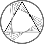
Figure 6: Example of a family of degenerate classical orbits in a circular billiard. The black triangular orbit can be rotated by an arbitrary angle without changing its length. All resulting orbits contribute the same to the density of states. (adapted from Ref. Brack and Bhaduri, 2008.)

a) circular infinite			b) square billiard		c) square billiard
mass billiard			(“semiconducting”)		(“metallic”)
TF	TF (P)	QM	TF	QM	TF	QM
1.49	1.57	1.43	6.85	6.81	6.86	6.85
2.72	2.78	2.63	7.85	7.84	7.30	7.28
3.10	3.14	3.11	7.93	7.87	7.92	7.85
3.87	3.92	3.77	8.11	8.05	8.15	8.09
4.46	4.49	4.48	8.97	8.92	8.41	8.39
4.69	4.71	4.68	9.11	9.10	8.84	8.80
5.00	5.04	4.88	9.26	9.24	9.43	-
5.73	5.75	5.75	9.35	9.32	9.54	9.50
6.10	6.12	5.98	10.47	-	9.85	9.85
6.10	6.14	6.09	10.86	10.86	10.06	10.05
6.26	6.28	6.27	10.92	10.90	10.59	10.56
6.95	6.98	6.98	11.05	11.01	11.04	11.00
7.20	7.23	7.06	11.18	11.14	11.04	11.03
7.43	7.45	7.41	11.29	11.27	11.21	11.16
7.71	7.72	7.71	11.52	-	11.71	11.69

Table 2: a) Energy levels $k_{n}R$ of the circular billiard with infinite mass type edges obtained from the semiclassical trace formula Eq. (IV.2.1) by summing over many classical orbits with $\xi=0$ (TF) and by summing up all orbits approximately (TF (P)) Eq. (87) compared to the quantum mechanical result (QM) Eq. (86). b), c) Energy levels $k_{n}L$ for square billiards with $KL\mod 2\pi=2\pi/3$ ($L=200\,a$ “semiconducting”) and $KL\mod 2\pi=0$ ($L=201\,a$ “metallic”), respectively. Again we compare the result from the semiclassical trace formula (IV.2.2) at $\xi=0$ with the quantum mechanical result (144).

IV.2.1 Circular billiard with infinite mass type edges

We begin with a circular billiard with infinite mass type edges. Then the quantum energy levels $E_{nm}=\hbar v_{\scriptscriptstyle F}k_{nm}$ are given by the intersections of Bessel functionsBerry (1985)

$$J_{n}(k_{nm}R)=\tau J_{n+1}(k_{nm}R)\,,$$ (86)

where $R$ is the billiard radius, $\tau=\pm 1$ labels the two valleys and $n,m\in\mathbb{Z}$, where $m$ counts the intersections.

For the semiclassical calculation of $\rho_{\text{osc}}$ we adapt results for the Schrödinger disk billiard as derived and discussed in detail e.g. in Ref. Brack and Bhaduri, 2008. Periodic orbit families in the disk are labeled by the total number of reflections $v$ and the winding number $w$, with $v\geq 2w$. Examples with $w=1,2$ are depicted in Fig. 7. We also allow for negative winding numbers $w$, and define the sign such that $w>0$ for clockwise going orbits and $w<0$ for anti-clockwise going orbits. Simple geometry gives for the length $L_{v,w}$ and the angle of rotation $\varphi_{v,w}$ aquired of an orbit $(v,w)$

$$L_{v,w} = 2vR\sin(|\varphi_{v,w}|)\,,$$ (87)

$$\varphi_{v,w} = \pi\frac{w}{v}\,.$$ (88)

Then the reflection angles read

$$\theta_{v,w}=\left(\frac{\text{sgn}(w)}{2}-\frac{w}{v}\right)\pi\,.$$ (89)

Graphene physics enters through the pseudospin propagator, Eq. (77), with boundary matrix

$$P_{\boldsymbol{\alpha}}=(1+\tau_{z}\otimes\sigma_{\boldsymbol{t_{\alpha}}})/2$$ (90)

for the infinite mass case [see Eq. (4) and Tab. 1  ]. For an orbit $(v,w)$ the trace over $K$ yields

$$\text{Tr}{K}_{v,w} = i^{v}\text{Tr}\left(\tau_{z}^{v}\otimes\sigma_{z}^{v}e^{iv\theta_{v,w}\sigma_{z}}\right)$$ (93)

$$= 4\cos(v\,\theta_{v,w})\left\{\begin{array}[]{cl}(-1)^{v/2}&\text{for~{}even~{}}v\,,\\ 0&\text{for~{}odd~{}}v\,.\end{array}\right.$$

Equation (93) reveals the interesting property that only orbits with an even number of reflections are contributing to the oscillating DOS in the circular graphene billiard, while for odd $v$, the pseudospins are interfering destructively. Note that this holds true also in each valley separately, because in the case of odd $v$, the contributions from winding numbers $w$ and $-w$ have opposite signs.

Adapting the expression for the circular Schrödinger billiardBrack and Bhaduri (2008); Bogachek and Gogadze (1973) accordingly yields the semiclassical expression for the oscillatory part of the DOS of the graphene disk:

$$\rho_{\text{osc}}^{\text{sc}}(k_{\scriptscriptstyle E}) = 4\sqrt{\frac{k_{\scriptscriptstyle E}R^{3}}{\pi}}\sum_{w=1}^{\infty}\sum_{\stackrel{{\scriptstyle\scriptstyle v=2w}}{{\text{even}}}}^{\infty}(-1)^{w+v/2}\frac{f_{v,w}}{\sqrt{v}}$$

$$\times\sin^{3/2}(\varphi_{v,w})\sin\left(k_{\scriptscriptstyle E}L_{v,w}+\frac{3}{4}\pi\right)e^{-(\xi L_{v,w}/2)^{2}}$$

where $f_{v,w}=1$ if $v=2w$ and otherwise $f_{v,w}=2$.

The last factor in Eq. (IV.2.1), giving rise to an exponential suppression of orbits of length $L_{v,w}>1/\xi$, represents a broadening of the peaks in the quantum density of states by convoluting $\rho$ with a Gaussian of width $\xi$. Such a broadening is additionally introduced to mimic e.g. temperature smearing or account for a finite life time of the quantum states, for instance due to residual disorder scatteringRichter1996 . Thereby, Eq. (IV.2.1) relates gross effects in smeared quantum spectra or experimental spectra obtained with limited resolution to the contributions from families of shortest periodic orbits Brack and Bhaduri (2008); Richter et al. (1996).

Using the Poisson summation formula, we can approximately sum up the trace formula (IV.2.1) for $\xi=0$ and find the approximate eigenenergies $k_{VW}=x_{VW}/R$ corresponding to poles in the semiclassical sum, that fulfill the equation

$$V+\frac{3}{2} = (2W+1)[1-\arccos(W/X_{VW})/\pi]$$ (95)

$$+\frac{2X_{VW}}{\pi}\sqrt{1-W^{2}/X_{VW}^{2}}-2W\,.$$

In Fig. 8 a)-c) we compare the results of the semiclassical trace formula (IV.2.1) with exact quantum results from Eq. (86) for the lower part of the graphene disk spectrum. For $\xi=0$ [panel a)] even the exact quantum levels (blue circles) are reproduced with remarkable accuracy by the semiclassical theory [black peaks, see also numerical values in Tab 2 a)]. For every level, we have a sharp peak in the semiclassical result. An exception are the two levels close to $k_{\scriptscriptstyle E}R=6$, for which we have only one peak, though twice as high as the others, meaning that in the semiclassical expression the two levels are nearly degenerate.

Panel b) shows the broadened spectrum for $\xi=0.3/R$. Again, the semiclassical result (solid line) is in very good agreement with the corresponding quantum result (dotted). For comparison, panel d) shows the same energy range for the corresponding Schrödinger billiard. In Fig. 8 c) we have a closer look at which orbit families contribute. In fact we can see from Fig. 8 c) that the two shortest non-vanishing orbit families $(2,1)$ and $(4,1)$ already yield a good approximation to the shell structure for $\xi=0.4/R$.

Fig. 9 shows the power spectrum of the exact quantum result (Gaussian convoluted with $\xi=0.4/R$). Evidently, only families with an even number of vertices $v$ are contained in the spectrum, as semiclassically predicted. For example the triangular orbits $(3,1)$ that would give a peak at $L/R=5.2$ and also the pentagram orbits $(5,2)$ ($L/R=9.5$) do not contribute. The inset shows the same plot on a logarithmic scale, where the absence of the odd orbits is even more evident.

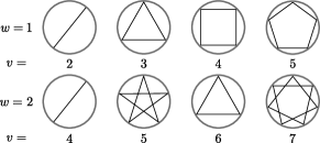
Figure 7: Classical periodic orbits representing families in the circular billiard. $v$ is the total number of reflections along the orbit and $w$ denotes the winding number. If ($v,w$) are not coprime the orbit is a repetition of a shorter primitive orbit. E. g. (4,2) is a repetition of (2,1) and (6,2) of (3,1). (Adapted from Ref. Balian and Bloch, 1972.)

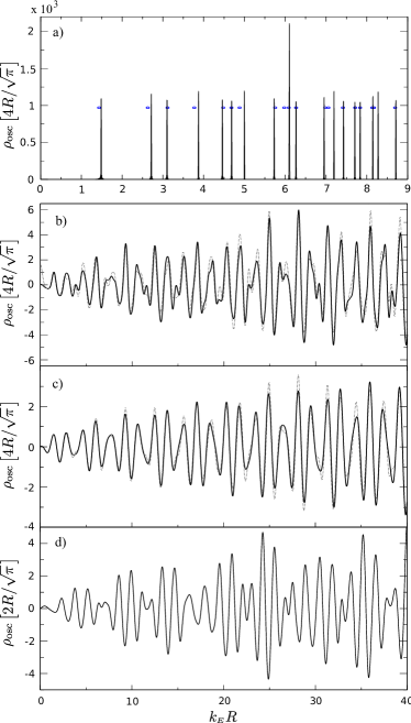
Figure 8: (color online). Oscillating part $\rho_{\text{osc}}$ of the density of states of a circular billiard as a function of $k_{\scriptscriptstyle E}R$. a) Peaks are obtained from the semiclassical expression (IV.2.1) by summing up orbit families up to $v,w=400$ for $\xi=0$. Blue circles mark the positions of the exact quantum mechanical levels given by Eq. (86) (See also Tab 2 a)). b) Gaussian convoluted $\rho_{\text{osc}}$ for $\xi=0.3/R$. The full (dotted) curves show the semiclassical (quantum mechanical) results. c) Comparison between the full semiclassical orbit sum (dotted, $\xi=0.4/R$) with the contribution from the two shortest orbit families $(2,1)$ and $(4,1)$ (solid). d) Corresponding results (for $\xi=0.4/R$) for a circular Schrödinger billiard with Dirichlet boundary conditions.

Figure 9: Power spectrum of the Gaussian convoluted ($\xi=0.3/R$) quantum density of states of the graphene disk with infinite mass edges. Peaks can be uniquely assigned to periodic orbit families $(v,w)$, see text. Inset: Logarithmic respresentation.

IV.2.2 Rectangular billiard with zigzag and armchair edges

Figure 10: Families of periodic classical orbits in the rectangular billiard. $N(M)$ is the number of reflections at the bottom (left) side.

The rectangular billiard represents another prominent classically integrable geometry. While for the Schrödinger equation with Dirichlet boundary conditions this is a simple textbook problem, there is no explicit expression for eigenenergies of the graphene rectangle with two opposite zigzag and two opposite armchair edges. (For the derivation of a closed formula for the quantum eigenenergies in terms of a transcendental equation see App. C). We will show that our semiclassical theory provides a very good approximation to the quantum density of states.

In the rectangle, the periodic orbit families can again be labeled with two indices. We denote by $N$ and $M$ the number of reflections at the bottom zigzag ($N$) and the left armchair ($M$) side of the rectangle with lengths $L_{x}$ and $L_{y}$ respectively (see Fig. 10). The absolute values of the reflection angles at the zigzag and armchair edges then read

$$\begin{split}&|\theta_{\text{zz}}|=\arctan\left(\frac{ML_{x}}{NL_{y}}\right)\,,\\ &|\theta_{\text{ac}}|=\frac{\pi}{2}-|\theta_{\text{zz}}|=\arctan\left(\frac{NL_{y}}{ML_{x}}\right)\,.\end{split}$$ (96)

From Eq. (83) we can read off the following matrix factors for reflections with angles $\theta_{\text{zz}}$ and $\theta_{\text{ac}}$, respectively:

$$\begin{split}-i\tau_{z}e^{-i\theta_{\text{zz}}\tau_{z}}\otimes\sigma_{x}&~{}~{}~{}~{}\text{lower zigzag edge,}\\ -i\tau_{z}e^{i\theta_{\text{zz}}\tau_{z}}\otimes\sigma_{x}&~{}~{}~{}~{}\text{upper zigzag edge,}\\ i\tau_{y}\otimes\sigma_{z}e^{i\theta_{\text{ac}}\sigma_{z}}&~{}~{}~{}~{}\text{left armchair edge,}\\ -i\tau_{y}e^{i2KL_{x}\tau_{z}}\otimes\sigma_{z}e^{i\theta_{\text{ac}}\sigma_{z}}&~{}~{}~{}~{}\text{right armchair edge}\,.\end{split}$$ (97)

This enables us to calculate the pseudospin trace of a periodic orbit from family $(N,M)$ as

$$\text{Tr}{K}_{NM}=(-1)^{N}4\cos(2MKL_{x}-2N|\theta_{\text{zz}}|)\,.$$ (98)

This expression holds irrespective of the propagation direction along the orbit. Note also that the $\theta_{\text{zz}}$ in Eq. (98) occurs only due to the fact that we have different zigzag edges at the top and the bottom boundary (A- and B-terminated, respectively). Equation (98) is now used to adapt the trace formula for the Schrödinger equation which has been derived e. g. in Refs. Brack and Bhaduri, 2008 and Richter et al., 1996 to the case of graphene. Taking into account the interfering pseudospins in graphene, we find

$$\rho_{\text{osc}}^{\text{sc}}(k_{\scriptscriptstyle E}) = \sqrt{\frac{k_{\scriptscriptstyle E}}{2\pi^{3}}}\sum_{M=1}^{\infty}\sum_{N=1}^{\infty}\frac{f_{NM}\,L_{x}L_{y}}{\sqrt{L_{NM}}}$$

$$\times\cos\left(k_{\scriptscriptstyle E}L_{NM}-\frac{\pi}{4}\right)\text{Tr}{K}_{NM}\,e^{-(\xi L_{NM}/2)^{2}}$$

with length $L_{NM}=2\sqrt{M^{2}L_{x}^{2}+N^{2}L_{y}^{2}}$ and $\text{Tr}{K}_{NM}$ from Eq. (98). Further $f_{NM}=1$ if $N=0$ or $M=0$ and otherwise $f_{NM}=2$. Note that the size of the billiard determines whether certain orbits contribute: The quantity $KL_{x}$ can only take values that are multiples of $\pi/3$. In particular for $KL_{x}=0\mod 2\pi$ note_3 , families $(N,NL_{y}/L_{x})$ with odd $N$ do not contribute according to Eq. (98). Further examples are the families $(M,0)$ and $(0,N)$ for odd $N$ and $M$ respectively. They cancel each other exactly for $KL_{x}=0\mod 2\pi$ because of the $(-1)^{N}$ term in the pseudospin trace.

In Fig. 11 and Tab 2 b), c) we compare the results from the semiclassical trace formula (IV.2.2) for $L_{x}=L_{y}=L$ with the quantum mechanical results obtained by solving Eq. (144) numerically. Again we find very good agreement with the quantum result. This is rather remarkable because of the complicated structure of the quantization condition (144). The semiclassical predictions concerning the frequency content of the DOS oscillations are confirmed in Fig. 11  c) and d). For example the shortest orbits $(1,0)$, $(0,1)$ and $(1,1)$ do not contribute for the system in d) ($KL\mod 2\pi=0$) due to destructive pseudospin interference, while they are important in c) ($KL\mod 2\pi=2\pi/3$).

Note that in Tab. 2 we find some additional levels from the semiclassical trace formula, which cannot be associated to quantum energy levels of the rectangle. Rather these peaks occur at positions that fulfill the quantization condition of a fictitious 1D quantum well of width $L$ with armchair boundary conditions. It is well knownBrack and Bhaduri (2008) that this is an effect of subleading order ($[k_{\scriptscriptstyle E}L]^{-1/2}$ with respect to leading order) produced by orbits that ‘graze’ along the edges.

Figure 11: Oscillating part of the density of states of a square billiard with two armchair edges and two zigzag edges ($L_{x}=L_{y}=L$). The left panels (a, c) show the results for a square with $KL\mod 2\pi=2\pi/3$ (“semiconducting”) and the right panels (b, d) are for a square with $KL\mod 2\pi=0$ (“metallic”). Panels a) and b) show the Gaussian convoluted $\rho_{\text{osc}}(k_{\scriptscriptstyle E})$ for $\xi=0.3/L$. The dotted curves represent the quantum mechanically exact results calculated with Eq. (144) and broadened correspondingly. Panels c) and d) show the quantum mechanical power spectra (for $\xi=0.3$). It is easy to identify the peaks associated with corresponding families $(M,N)$.

IV.3 Trace formula for classically chaotic graphene billiards

Finally we consider classically chaotic graphene systems. In this case no spatial symmetries are present that would give rise to an orbit degeneracy as in the regular case. From Eq. (78) we already know that the final result differs from the trace formula for chaotic Schrödinger billiards only with respect to the pseudospin trace. Thus we have to work out how the spatial integral in Eq. (6) depends on this trace. To this end we do not start directly from the semiclassical Green’s function (76), but go one step back to Eq. (73). In order to calculate the integral

$$\rho_{N}(k_{\scriptscriptstyle E})=-\frac{1}{\pi}\mathfrak{Im}\int\limits_{\mathcal{V}}\!d\boldsymbol{x}\,\text{Tr}\left[G_{N}(\boldsymbol{x},\boldsymbol{x})\right]$$ (100)

we consider only the $\boldsymbol{x}$-dependent part of the integrand,

$$I_{N}=\int\limits_{\mathcal{V}}\!d\boldsymbol{x}\,\frac{K(\boldsymbol{x},\underline{\boldsymbol{\alpha}})}{\sqrt{|\boldsymbol{x}-\boldsymbol{\alpha}_{N}||\boldsymbol{\alpha}_{1}-\boldsymbol{x}|}}e^{ik_{\scriptscriptstyle E}(|\boldsymbol{x}-\boldsymbol{\alpha}_{N}|+|\boldsymbol{\alpha}_{1}-\boldsymbol{x}|)}\,,$$ (101)

and choose the parametrization $\boldsymbol{x}=l\,\hat{\boldsymbol{l}}+t\,\hat{\boldsymbol{t}}$, where $\hat{\boldsymbol{l}}$ is the direction from $\boldsymbol{\alpha}_{N}$ to $\boldsymbol{\alpha}_{1}$ and $\hat{\boldsymbol{t}}$ the direction perpendicular to $\hat{\boldsymbol{l}}$ such that a right handed coordinate system results. The origin $l=t=0$ is at the point $\boldsymbol{\alpha}_{N}$ and we denote $l_{N1}=|\boldsymbol{\alpha}_{N}-\boldsymbol{\alpha}_{1}|$. Then we can rewrite the phase

$$\varphi(l,t)/k_{\scriptscriptstyle E}\!\!\!\!\! = \!\!\!\!\!|\boldsymbol{x}-\boldsymbol{\alpha}_{N}|+|\boldsymbol{\alpha}_{1}-\boldsymbol{x}|$$ (102)

$$\stackrel{{\scriptstyle t\ll l,l-l_{N1}}}{{\approx}} l_{N1}\left(1+\frac{t^{2}}{2l[l_{N1}-l]}\right)\,.$$

We are now evaluating the $t$-integral in stationary phase approximation assuming $k_{\scriptscriptstyle E}l_{N1}\gg 1$. The stationary phase point $t_{0}$ is given by

$$\frac{\partial\varphi(l,t_{0})}{\partial t} = \frac{k_{\scriptscriptstyle E}\,l_{N1}t_{0}}{l(l_{N1}-l)}=0\quad\Rightarrow\quad t_{0}=0\,,$$ (103)

$$\frac{\partial^{2}\varphi(l,t_{0})}{\partial t^{2}} = \frac{k_{\scriptscriptstyle E}\,l_{N1}}{l(l_{N1}-l)}\,,$$ (104)

$$\quad\varphi(l,t_{0}) = k_{\scriptscriptstyle E}\,l_{N1}=k_{\scriptscriptstyle E}\,|\boldsymbol{\alpha}_{N}-\boldsymbol{\alpha}_{1}|\,.$$ (105)

This means however that at the critical point $t_{0}$, the pseudospin propagator $K(\underline{\boldsymbol{\alpha}})$ has no dependence on $l$ left, since for $t=0$ Eq. (85) holds. Thus the remaining integral can be performed exactly:

$$I_{N}=\sqrt{\frac{2\pi l_{N1}}{k_{\scriptscriptstyle E}}}K(\underline{\boldsymbol{\alpha}})\,e^{ik_{\scriptscriptstyle E}\,|\boldsymbol{\alpha}_{N}-\boldsymbol{\alpha}_{1}|}\,.$$ (106)

This tells us that as for the Green’s function, we can essentially read off the result for $\rho_{\text{osc}}^{\text{sc}}$ directly from the corresponding Dirichlet problem for the Schrödinger equationGutzwiller (1990) and find the Gutzwiller-type trace formula for a chaotic graphene cavity

$$\rho_{\text{osc}}^{\text{sc}}(k_{\scriptscriptstyle E})=\frac{v_{\scriptscriptstyle F}}{2\pi}\mathfrak{Re}\sum_{\gamma}\text{Tr}(K_{\gamma})A_{\gamma}\,e^{ik_{\scriptscriptstyle E}L_{\gamma}}\,.$$ (107)

Here the sum runs over all, infinitely many classical periodic orbits $\gamma$, because the stationary phase points with $t=t_{0}=0$ are lying exactly on the straight line connecting the last with the first reflection point, i. e. the apperance of the pseudospin does not affect the stationary points. The classical amplitudes $A_{\gamma}$ depend on the period, the stability and the Maslov index of the corresponding orbitGutzwiller (1990). That means, except for $\hbar$ and the trace over $K_{\gamma}$, accounting for the interference of pseudospins, the right-hand side of Eq. (107) contains only classical quantities and has the same structure as Gutzwiller’s trace formula. We note that in Ref. Carmier and Ullmo, 2008 a semiclassical trace formula is presented for $\rho_{\text{osc}}$, which however is not taking into account the boundaries required to obtain chaotic dynamics. Note that the expression (107) for $\rho_{\text{osc}}$ is only valid for systems with isolated orbits, a prerequisite to evaluate the integral perpendicular to $\boldsymbol{\alpha}_{N}-\boldsymbol{\alpha}_{1}$ in stationary phase approximation. This is particularly fulfilled for chaotic systems.

Expression (107) allows, in principle, for computing semiclassical approximations for energy levels in chaotic graphene billiards. We presume that this trace formula holds true more generally for classically chaotic graphene systems, not only billiards, with an appropriate generalization of the pseudospin evolution. Since the classical dynamics of a graphene billiard is the same as that of a Schrödinger billiard, the convergence properties of Eq. (107) are expected to be similar to those of Gutzwiller’s trace formula, with convergence problems linked to the exponential proliferation of periodic orbits with their length. In App. D, we discuss the effect of weak bulk disorder on the trace formula (107).

As Gutzwiller’s trace formula for the case of quantum chaotic Schrödinger dynamics, the trace formula (107) represents a suitable starting point to consider the statistical properties of energy levels for chaotic graphene cavities, in particular universal spectral features within certain symmetry classes. Based on Eq. (107) we devote a major part of Ref. partII to the semiclassical analysis of spectral statstics in graphene. There we will see that intervalley scattering, semiclassically incorporated in the pseudospin dynamics, plays a key role for the effective symmetry class obeyed in graphene, e. g. unitary, orthogonal or intermediate statistics between the two.

V Conclusion

The growing ability to manufacture graphene-based nanostructures and their increasing role in the field of graphene physics poses challenges to theory to treat confinement effects. Addressing ballistic graphene cavities we have focussed on the effect of different types of edges, zigzag, armchair and inifinite mass type, on the spectral properties. The multiple reflection expansion used, combined with the semiclassical approximation, allows for incorporating and analyzing edge phenomena in a particularly transparent way, both for the mean density of states $\bar{\rho}$ as well as for the remaining oscillatory part: The leading-order Weyl contribution to $\bar{\rho}$ for graphene billiards scales with the phase space volume on the energy shell, as for Schrödinger-type billiards. Edge effects are expected to alter the perimeter correction to $\bar{\rho}$, which is proportional to the total boundary length in the Schrödinger case with Dirichlet boundary conditions. We showed for graphene billiards that armchair and infinite mass edges do not give any perimeter contribution, while zigzag edges yield a characteristic low-energy term scaling with the length of the zigzag boundary. As analyzed in detail we could relate this boundary term in $\bar{\rho}$ to the average number of quantum zigzag edge states. Thereby, our approach allows for an alternative, analytical calculation of the zigzag edge state contribution. For graphene nanostructures with unknown portion of zigzag-type edge segments, this enables one to estimate the effective zigzag edge length, respectively number of edge states, from the characteristic feature in $\bar{\rho}(E)$, see Figs. 4 and 3. Hence, already the mean density of states of graphene flakes incorporates important physical information.

For the oscillatory contribution, $\rho_{\rm osc}$, to the density of states of graphene billiards we derive semiclassical trace formulae in terms of sums over classical periodic orbits. We show that, within the leading-order semiclassical approximation, the classical orbital dynamics entering into the semiclassical sums is the same as for Schrödinger billiards of the same geometry. This implies for regular graphene geometries Berry-Tabor like Berry1976/77 sums over families of orbits and for chaotic geometries a Gutzwiller type Gutzwiller (1990) trace formula in terms of isolated periodic trajectories. Edge effects enter into the contribution of each periodic orbit (family) exclusively through the the pseudospin propagator and its trace along the orbit. This leads to a particularly transparent representation of graphene edge phenomena. We gave a detailed interpretation for two representative regular systems: the graphene disk with infinite mass edges and the graphene 2d box with boundaries built from two zigzag and two armchair edges. The comparison with full quantum results showed very good agreement, both for smeared spectra, highlighing the role of short, fundamental periodic orbits, and on the level of individual energy levels, obtained semiclassically by summing up many orbit families.

A number of questions and further research directions is now arising from this work. They include the challenge to generalize the semiclassical expressions for the density of states of clean billiards to cavities with impurity scattering and systems with smooth confinement potentials, more generally graphene with arbitrary classical Hamiltonian dynamics, including also systems with mixed phase space. Second, the fact that our treatment of the zigzag edge associated average level density proofs adequate for both settings, models without and with particle-hole breaking effects, e.g. from next-nearest-neighbor coupling, see Sec. III.3.2, encourages to address zigzag edge magnetism Fujita et al. (1996); Wimmer et al. (2008); Son2006 ; Tao2011 within this framework. Third, the semiclassical formalism developed allows for treating graphene nanostructures with boundaries that can be viewed of being composed of many zigzag- and armchair-edge segments. In particular, analytical expressions can be derived by treating long orbits with bounces off the different boundary segments in a statistical way. Fourth, the techniques used can be generalized to quantum transport through open graphene nanostructures.

In a second paper partII we will particularly address the two last items and study spectral statistics (through the spectral form factor) of closed systems and transport properties (weak localization, universal conductance fluctuations and shot noise) of open graphene billiards.

VI Acknowledgements

We thank Philippe Jacquod, Viktor Krückl, Jack Kuipers, Juan Diego Urbina and Michael Wimmer for useful conversations. We acknowledge funding through the Deutsche Forschungsgemeinschaft within DFG Research Training Group 1570 (KR, JW) and through TUBA under grant I.A/TUBA-GEBIP/2010-1 and the funds of the Erdal İnönü chair at Sabancı University (IA). JW further acknowledges the support and hospitality at Sabancı University.

Appendix A The singularity of a Dirac-charge layer

Here we derive the expression (II) inducting the discontinuity of the Green’s function at the boundaryAdagideli and Goldbart (2002). Using the short distance asymptotic form for the Hankel function

$$H_{0}^{+}(\xi)\stackrel{{\scriptstyle\xi\ll 1}}{{\longrightarrow}}\frac{2i}{\pi}\ln(\xi/2)\,,$$ (108)

we obtain the short range singularities of the free Green’s function from Eq. (10)

$$G_{0}(\boldsymbol{x},\boldsymbol{x}^{\prime})\stackrel{{\scriptstyle\boldsymbol{x}\rightarrow\boldsymbol{x}^{\prime}}}{{\longrightarrow}}-\frac{i}{2\pi}\frac{\boldsymbol{\sigma}\cdot(\boldsymbol{x}-\boldsymbol{x}^{\prime})}{|\boldsymbol{x}-\boldsymbol{x}^{\prime}|^{2}}\,.$$ (109)

If $\boldsymbol{x}^{\prime}$ lies in the interior of $\mathcal{V}$ and $\boldsymbol{\alpha}$ is a point on the boundary $\partial\mathcal{V}$,

$$\lim_{\boldsymbol{x}\rightarrow\boldsymbol{\alpha}}G_{0}(\boldsymbol{x},\boldsymbol{x}^{\prime})=G_{0}(\boldsymbol{\alpha},\boldsymbol{x}^{\prime})$$ (110)

is well defined and the first term in Eq. (II) is trivially obtained from Eq. (9). However if $\boldsymbol{x}^{\prime}$ is on the boundary, the singular behavior of the Green’s function becomes relevant. To see this, we perform the boundary integral in two parts, dividing $\partial\mathcal{V}$ into a small region $D_{\delta}(\boldsymbol{\alpha})=C_{\delta}(\boldsymbol{\alpha})\bigcap\partial\mathcal{V}$, where $C_{\delta}(\boldsymbol{\alpha})$ is a circle with radius $\delta$ around $\boldsymbol{\alpha}$, and the remaining border $\bar{D}_{\delta}(\boldsymbol{\alpha})=\partial\mathcal{V}\setminus D_{\delta}(\boldsymbol{\alpha})$. We will take the limit $\delta\rightarrow 0$ at the end of the calculation.

We begin with the integration within $D_{\delta}(\boldsymbol{\alpha})$. To this end we use the asymptotic expression for $G_{0}$ and get

$$I_{D_{\delta}(\boldsymbol{\alpha})} = \lim_{\delta\rightarrow 0}\lim_{\boldsymbol{x}\rightarrow\boldsymbol{\alpha}}\int\limits_{D_{\delta}(\boldsymbol{\alpha})}\!\!\!d\sigma_{\boldsymbol{\beta}}G_{0}(\boldsymbol{x},\boldsymbol{\beta})i\sigma_{\boldsymbol{n_{\beta}}}\mu({\boldsymbol{\beta},\boldsymbol{x}^{\prime}})$$

$$= \frac{\sigma_{\boldsymbol{n_{\beta}}}}{2\pi}\mu({\boldsymbol{\alpha},\boldsymbol{x}^{\prime}})\boldsymbol{\sigma}\cdot\lim_{\delta\rightarrow 0}\lim_{\boldsymbol{x}\rightarrow\boldsymbol{\alpha}}\int\limits_{D_{\delta}(\boldsymbol{\alpha})}\!\!\!d\sigma_{\boldsymbol{\beta}}\frac{(\boldsymbol{x}-\boldsymbol{\beta})}{|\boldsymbol{x}-\boldsymbol{\beta}|^{2}}~{},$$

where we took $\mu$ out of the integral and evaluated it at $\boldsymbol{\beta}=\boldsymbol{\alpha}$. Without loss of generality, we choose $\boldsymbol{\alpha}=\boldsymbol{0}$, $\boldsymbol{x}=|\boldsymbol{x}|\hat{\boldsymbol{y}}$ and approximate $D_{\delta}(\boldsymbol{\alpha})$ by a straight line along the $x$-axis, i. e. $D_{\delta}(\boldsymbol{\alpha})~{}=~{}\{~{}\xi\hat{\boldsymbol{x}}~{}|~{}\xi\in[-\delta,\delta]~{}\}$. Then we get

$$I_{D_{\delta}(\boldsymbol{\alpha})} = \frac{\sigma_{\boldsymbol{n_{\beta}}}}{2\pi}\mu({\boldsymbol{\alpha},\boldsymbol{x}^{\prime}})\boldsymbol{\sigma}\cdot\lim_{\delta\rightarrow 0}\lim_{|\boldsymbol{x}|\rightarrow 0}\int\limits_{-\delta}^{\delta}d\xi\frac{|\boldsymbol{x}|\hat{\boldsymbol{y}}-\xi\hat{\boldsymbol{x}}}{|\boldsymbol{x}|^{2}+\xi^{2}}$$ (112)

$$= \frac{\sigma_{\boldsymbol{n_{\beta}}}}{2\pi}\mu({\boldsymbol{\alpha},\boldsymbol{x}^{\prime}})\boldsymbol{\sigma}\cdot\lim_{\delta\rightarrow 0}\lim_{|\boldsymbol{x}|\rightarrow 0}2\arctan(\delta/|\boldsymbol{x}|)\hat{\boldsymbol{y}}$$

$$= \frac{1}{2}\mu(\boldsymbol{\alpha},\boldsymbol{x}^{\prime})~{}.$$

Since the kernel of the integral on $\bar{D}_{\delta}(\boldsymbol{\alpha})$ has no singularity, it simply follows

$$\lim_{\delta\rightarrow 0}\lim\limits_{\boldsymbol{x}\rightarrow\boldsymbol{\alpha}} \!\!\!\!\!\!\!\!\int\limits_{\bar{D}_{\delta}(\boldsymbol{\alpha})}d\sigma_{\boldsymbol{\beta}}G_{0}(\boldsymbol{x},\boldsymbol{\beta})i\sigma_{\boldsymbol{n_{\beta}}}\mu({\boldsymbol{\beta},\boldsymbol{x}^{\prime}})$$ (113)

$$= \int\limits_{\partial V}d\sigma_{\boldsymbol{\beta}}G_{0}(\boldsymbol{\alpha},\boldsymbol{\beta})i\sigma_{\boldsymbol{n_{\beta}}}\mu({\boldsymbol{\beta},\boldsymbol{x}^{\prime}})~{}.$$

It is known from potential theory, that the integral on the right hand side existsBalian and Bloch (1970) and thus Eq. (II) follows.

Appendix B Effective boundary condition for zigzag edges in the presence of next-nearest neighbor hopping

It has been shown in Refs. Wimmer, 2008 and Sasaki et al., 2009 that the inclusion of next-nearest-neighbor (nnn) hopping in the tight-binding Hamiltonian of graphene has important consequences on the properties of the zigzag edge states. While for bulk graphene, up to a constant energy shift, the effects are of subleading order in $k$, for finite samples nnn hopping leads to an additional effective potential that is located solely on the edge atoms, therefore leading to qualitative changes of the edge state properties. These range from a finite dispersion to a complete change of the current profile in transportWimmer (2008) .

Here we neglect terms of higher order in $k$ in the Hamiltonian due to the nnn hopping and focus on the effects of the resulting edge potential. To this end we derive an effective boundary condition for the Dirac Hamiltonian with zigzag boundary. We consider a single zigzag edge, where the last row of atoms is located at $y_{0}=a/\sqrt{3}$. Furthermore the graphene flake shall be extended for $y>y_{0}$, i. e. the last row of atoms is of $B$-type. The Hamiltonian is then given bySasaki et al. (2009)

$$\mathcal{H}=v_{\scriptscriptstyle F}\boldsymbol{\sigma}\!\cdot\!\boldsymbol{p}-\hbar v_{\scriptscriptstyle F}\frac{t^{\prime}}{2}\delta(y-y_{0})(1-\sigma_{z}\otimes\tau_{z})\,.$$ (114)

Here $t^{\prime}\approx 0.1$ is the ratio of the next-nearest neighbor hopping constant, and the projection $(1-\sigma_{z}\otimes\tau_{z})$ ensures that the potential is located on the $B$-sublattice. Similar edge potentials can model also adsorbants at graphene edges or edge magnetism Wimmer et al. (2010, 2008).

The Dirac equation together with the Bloch theorem gives for the $y$-dependent part of the wavefunctions in the valley $\tau=+1$

$$k_{\scriptscriptstyle E}\psi_{A}(y) = k\psi_{B}(y)-\frac{\partial\psi_{B}(y)}{\partial y}\,,$$ (115)

$$k_{\scriptscriptstyle E}\psi_{B}(y) = k\psi_{B}(y)+\frac{\partial\psi_{A}(y)}{\partial y}-t^{\prime}\delta(y-y_{0})\psi_{B}(y)\,.$$

Now we integrate these equations over a small window $[y_{0}-\varepsilon,y_{0}+\varepsilon]$ around the potential and take the limit $\varepsilon\rightarrow 0$ afterwards. Assuming that $\psi$ has at most a finite discontinuity at $y_{0}$, we obtain from Eq. (115)

$$\lim_{\varepsilon_{0}\rightarrow 0^{+}}\psi_{B}(y+\varepsilon)-\psi_{B}(y_{0}-\varepsilon)=0\,,$$ (117)

i. e. the $B-$part of the spinor is continous. Thus we devide Eq. (B) by $\psi_{B}(y)$ before integrating and get

$$t^{\prime} = \lim_{\varepsilon\rightarrow 0^{+}}\int\limits_{y_{0}-\varepsilon}^{y_{0}+\varepsilon}\frac{1}{\psi_{B}(y)}\frac{\partial\psi_{A}(y)}{\partial y}$$ (118)

$$= \lim_{\varepsilon\rightarrow 0^{+}}\left[\frac{\psi_{A}(y_{0}+\varepsilon)}{\psi_{B}(y_{0}+\varepsilon)}-\frac{\psi_{A}(y_{0}-\varepsilon)}{\psi_{B}(y_{0}-\varepsilon)}\right]$$ (119)

using integration by parts. For $y<y_{0}$ we employ the actual zigzag boundary condition $\psi_{A}(0)=0$, leading to the known expressions for the wavefunctions for $y<y_{0}$Brey and Fertig (2006a); Wurm et al. (2009b):

$$\psi_{A}(y) = A\sin(qy)\,,$$

$$\psi_{B}(y) = \frac{A}{k_{\scriptscriptstyle E}}\left[ik\tau\sin(qy)+q\cos(qy)\right]\,,$$ (120)

with longitudinal and transverse momenta $k$ and $q$, respectively. Since the effective Dirac equation is valid for momenta that are much smaller than $1/a$, we approximate $k_{\scriptscriptstyle E}a,qa,ka\approx 0$ to get

$$\lim_{\varepsilon\rightarrow 0^{+}}\frac{\psi_{A}(y_{0}-\varepsilon)}{\psi_{B}(y_{0}-\varepsilon)}=\frac{k_{\scriptscriptstyle E}\sin(qa/\sqrt{3})}{ik\sin(qa/\sqrt{3})+q\cos(qa/\sqrt{3})}\approx 0\,,$$ (121)

which inserted into Eq. (119) finally leads to the effective boundary condition

$$\left.\frac{\psi_{A}}{\psi_{B}}\right|_{\partial\mathcal{V}}=t^{\prime}\,.$$ (122)

in agreement with a result found for similar edge potentials in Ref. Bhowmick2010, . In an analogous way one can derive the effective boundary condition for the other valley as well as for $A$-terminated zigzag edges to end up with an effective boundary condition matrix

$$P_{\boldsymbol{\alpha}}=\frac{1}{2}\left(1\mp\tau_{z}\otimes\sigma_{z}-it^{\prime}\sigma_{y}\pm t^{\prime}\tau_{z}\otimes\sigma_{x}\right)$$ (123)

for all points at the edge $\boldsymbol{\alpha}$. This expression turns into the usual zigzag matrix (29) when $t^{\prime}=0$.

We further derive the edge state dispersion and wavefunction from the Dirac equation with the effective boundary condition

$$\psi_{A}(0)=t^{\prime}\psi_{B}(0)\,.$$ (124)

Due to the Bloch theorem we can write for $k_{\scriptscriptstyle E}^{2}=k^{2}+q^{2}$

$$\Psi_{A}(x,y)=e^{ikx}\psi_{A}(y)=e^{ikx}(Ae^{iqy}+Be^{-iqy})$$ (125)

and

$$\psi_{B}(y)=(\tau k+\partial_{y})\psi_{A}(y)\,.$$ (126)

For nonzero $k_{\scriptscriptstyle E}$, Eq. (124) then leads to the condition

$$A(k_{\scriptscriptstyle E}-t^{\prime}\tau k-it^{\prime}q)=-B(k_{\scriptscriptstyle E}-t^{\prime}\tau k+it^{\prime}q)\,.$$ (127)

The bulk states result from this equation, when both sides are nonzero. On the other hand the edge state results if this is not the case, e. g. $k_{\scriptscriptstyle E}-t^{\prime}\tau k+it^{\prime}q=0$. Solving this equation gives for negative $\tau k$ the edge state

$$\Psi_{A}(x,y)\approx Be^{ikx}e^{\tau ky}\qquad\Psi_{B}(x,y)\approx B\frac{2k}{k_{\scriptscriptstyle E}}e^{ikx}e^{\tau ky}$$ (128)

with the dispersion relation

$$k_{\scriptscriptstyle E}^{\text{edge}}=\frac{2kt^{\prime}\tau}{1+t^{\prime 2}}\approx 2kt^{\prime}\tau\,.$$ (129)

This state exists only for negative (positive) momenta $k$ in the valley $K(K^{\prime})$ (as for the case without nnn hopping) and has always a negative energy.

Appendix C Energy eigenvalues of a rectangular graphene flake

Here we present an implicit expression for the energy eigenvalues of a graphene rectangle with zigzag edges at $y=0$ and $y=L_{y}$ and armchair edges at $x=0$ and $x=L_{x}$, respectively. To this end we start from a superposition of a forward and a backward propagating eigenmode of an armchair nanoribbon with edges at $x=0$ and $x=L_{x}$ Brey and Fertig (2006a); Wurm et al. (2009b),

$$\Psi(x,y) = A\left(\begin{array}[]{c}(q_{m}-ik)e^{iq_{m}x}\\ k_{\scriptscriptstyle E}e^{iq_{m}x}\\ k_{\scriptscriptstyle E}e^{-iq_{m}x}\\ (-q_{m}+ik)e^{-iq_{m}x}\end{array}\right)e^{iky}$$ (134)

$$+ B\left(\begin{array}[]{c}(q_{m}+ik)e^{iq_{m}x}\\ k_{\scriptscriptstyle E}e^{iq_{m}x}\\ k_{\scriptscriptstyle E}e^{-iq_{m}x}\\ (-q_{m}-ik)e^{-iq_{m}x}\end{array}\right)e^{-iky}$$ (139)

where the $q_{m}$ are quantized according to

$$q_{m}=\frac{m\pi}{L_{x}}-K\quad m\in\mathbb{Z}\,.$$ (140)

The spinors in Eq. (134) are solutions to the Dirac equation when

$$k^{2}+q_{m}^{2}=k_{\scriptscriptstyle E}^{2}\,.$$ (141)

Now we impose the zigzag boundary conditions $\Psi_{A}(x,0)=\Psi_{A^{\prime}}(x,0)=\Psi_{B}(x,L_{y})=\Psi_{B^{\prime}}(x,L_{y})=0$, which result in the two independent equations

$$(q_{m}-ik)A+(q_{m}+ik)B = 0\,,$$ (142)

$$e^{ikL_{y}}A+e^{-ikL_{y}}B = 0\,.$$ (143)

These are solved for quantized $k_{nm}$ that fulfill the transcendental equation

$$k_{nm}=-q_{m}\tan(k_{nm}L_{y})\,.$$ (144)

With that we have formally solved the problem, the eigenenergies can be found e. g. by solving Eq. (144) numerically.

Appendix D Effect of weak bulk disorder

At this point we briefly discuss the effect on the trace formula (107) caused by smooth bulk disorder, which can be accounted for by an additional term

$$H^{\prime}=\tau_{0}\otimes\sigma_{0}V(\boldsymbol{x})$$ (145)

in the Hamiltonian, where $V(\boldsymbol{x})$ is smooth on the scale of the lattice constantSuzuura2002 . In the semiclassical limit the Green’s function for $H+H^{\prime}$ has been derived in Ref. Carmier and Ullmo, 2008 without taking into account the boundaries. For the case of a Gaussian correlated disorder potential,

$$\left<V(\boldsymbol{x})V(\boldsymbol{x}^{\prime})\right>=C_{0}\exp\left[{-\frac{(\boldsymbol{x}-\boldsymbol{x}^{\prime})^{2}}{4\Delta^{2}}}\right]\,,$$ (146)

quantum calculations in the Boltzmann limit have been performed Adam2009 ; Vasko2010 . Under the assumption that the disorder potential is weak enough that the classical trajectories remain unaffected, we get for the impurity averaged Green’s functionRichter1996

$$\left<G_{0}^{\prime\text{sc}}(\boldsymbol{x},\boldsymbol{x}^{\prime})\right>\approx G_{0}^{\text{sc}}(\boldsymbol{x},\boldsymbol{x}^{\prime})\exp\left(-\left<\delta S^{2}\right>/2\hbar^{2}\right)$$ (147)

with

$$\left<\delta S^{2}\right> = \frac{1}{(2v_{\scriptscriptstyle F}k_{\scriptscriptstyle E})^{2}}\int\limits_{\boldsymbol{x}^{\prime}}^{\boldsymbol{x}}dq\int\limits_{\boldsymbol{x}^{\prime}}^{\boldsymbol{x}}dq^{\prime}\left<\left[(\boldsymbol{x}-\boldsymbol{x}^{\prime})\times\boldsymbol{\nabla}V(\boldsymbol{q})\right]\right.$$ (148)

$$\times\left.\left[(\boldsymbol{x}-\boldsymbol{x}^{\prime})\times\boldsymbol{\nabla}V(\boldsymbol{q}^{\prime})\right]\right>/|\boldsymbol{x}-\boldsymbol{x}^{\prime}|^{2}$$

$$\approx \hbar^{2}|\boldsymbol{x}-\boldsymbol{x}^{\prime}|/l$$ (149)

and the mean free path

$$l=\frac{4\Delta\hbar^{2}v_{\scriptscriptstyle F}^{2}k_{\scriptscriptstyle E}^{2}}{\sqrt{\pi}C_{0}}\,.$$ (150)

For smooth potentials the jump of the Green’s function in Eq. (II) and hence also the MRE (16) remains unchanged, except that $G_{0}$ has to be replaced by its impurity averaged version (147). Thus each summand in the semiclassical Green’s function (78) for a graphene cavity aquires a damping factor $e^{-L_{\gamma}/2l}$. In the trace integral (101), these factors do not alter the stationary phase points, so that also in the trace formula in (107) every periodic orbit contribution is weighted with a factor $e^{-L_{\gamma}/2l}$ that improves convergence of the semiclassical trace formula.

References

- Novoselov et al. (2004) K. S. Novoselov, A. K. Geim, S. V. Morozov, D. Jiang, Y. Zhang, S. Dubonos, I. Grigorieva, and A. Firsov, Science 306, 666 (2004).
- Novoselov et al. (2005) K. S. Novoselov, D. Jiang, F. Schedin, T. J. Booth, V. V. Khotkevich, S. V. Morozov, and A. K. Geim, Proc. Natl. Acad. Sci. U.S.A. 102, 10451 (2005).
- Geim and Novoselov (2007) A. K. Geim and K. S. Novoselov, Nature Mater. 6, 183 (2007).
- Avouris et al. (2007) P. Avouris, Z. Chen, and V. Perebeinos, Nature Nanotech. 2, 605 (2007).
- Beenakker (2008) C. W. J. Beenakker, Rev. Mod. Phys. 80, 1337 (2008).
- Castro Neto et al. (2009) A. H. Castro Neto, F. Guinea, N. M. R. Peres, K. S. Novoselov, and A. K. Geim, Rev. Mod. Phys. 81, 109 (2009).
- Abergel et al. (2010) D. Abergel, V. Apalkov, J. Berashevich, K. Ziegler, and T. Chakraborty, Adv. Phys. 59, 261–482 (2010).
- Han et al. (2007) M. Y. Han, B. Özyilmaz, Y. Zhang, and P. Kim, Phys. Rev. Lett. 98, 206805 (2007).
- Li et al. (2008) X. Li, X. Wang, L. Zhang, S. Lee, and H. Dai, Science 319, 1229 (2008).
- Tapaszto et al. (2008) L. Tapaszto, G. Dobrik, P. Lambin, and L. Biro, Nature Nanotech. 3, 397 (2008).
- Gallagher et al. (2010) P. Gallagher, K. Todd, and D. Goldhaber-Gordon, Phys. Rev. B 81, 115409 (2010).
- Ponomarenko et al. (2008) L. A. Ponomarenko, F. Schedin, M. I. Katsnelson, R. Yang, E. W. Hill, K. S. Novoselov, and A. K. Geim, Science 320, 356 (2008).
- Güttinger et al. (2008) J. Güttinger, C. Stampfer, S. Hellmüller, F. Molitor, T. Ihn, and K. Ensslin, Appl. Phys. Lett. 93, 212102 (2008).
- Güttinger et al. (2010) J. Güttinger, T. Frey, C. Stampfer, T. Ihn, and K. Ensslin, Phys. Rev. Lett. 105, 116801 (2010).
- (15) S. Russo, J. B. Oostinga, D. Wehenkel, H. B. Heersche, S. S. Sobhani, L. M. K. Vandersypen, and A. F. Morpurgo, Phys. Rev. B 77, 085413 (2008).
- (16) M. Huefner, F. Molitor, A. Jacobsen, A. Pioda, C. Stampfer, K. Ensslin, and T. Ihn, New J. Phys 12, 043054 (2010).
- Eroms and Weiss (2009) J. Eroms and D. Weiss, New J. Phys. 11, 095021 (2009).
- Bai et al. (2010) J. Bai, X. Zhong, S. Jiang, Y. Huang, and X. Duan, Nature Nanotech. 5, 190 (2010).
- Fujita et al. (1996) M. Fujita, K. Wakabayashi, K. Nakada, and K. Kusakabe, J. Phys. Soc. Jpn. 65, 1920 (1996).
- Nakada et al. (1996) K. Nakada, M. Fujita, G. Dresselhaus, and M. S. Dresselhaus, Phys. Rev. B 54, 17954 (1996).
- Brey and Fertig (2006a) L. Brey and H. A. Fertig, Phys. Rev. B 73, 235411 (2006a).
- (22) J. Tworzydło, B. Trauzettel, M. Titov, A. Rycerz, and C. W. J. Beenakker, Phys. Rev. Lett. 96, 246802 (2006).
- Silvestrov and Efetov (2007) P. G. Silvestrov and K. B. Efetov, Phys. Rev. Lett. 98, 016802 (2007).
- Trauzettel et al. (2007) B. Trauzettel, D. V. Bulaev, D. Loss, and G. Burkard, Nature Phys. 3, 192 (2007).
- (25) P. Recher, J. Nilsson, G. Burkard, and B. Trauzettel, Phys. Rev. B 79, 085407 (2009).
- (26) J. H. Bardarson, M. Titov, and P. W. Brouwer, Phys. Rev. Lett. 102, 226803 (2009).
- Libisch et al. (2009) F. Libisch, C. Stampfer, and J. Burgdörfer, Phys. Rev. B 79, 115423 (2009).
- Wurm et al. (2009a) J. Wurm, A. Rycerz, İ. Adagideli, M. Wimmer, K. Richter, and H. U. Baranger, Phys. Rev. Lett. 102, 056806 (2009a).
- Wimmer et al. (2010) M. Wimmer, A. R. Akhmerov, and F. Guinea, Phys. Rev. B 82, 045409 (2010).
- (30) P. Recher, B. Trauzettel, A. Rycerz, Ya. M. Blanter, C. W. J. Beenakker, and A. F. Morpurgo, Phys. Rev. B 76, 235404 (2007).
- (31) J. Wurm, M. Wimmer, H. U. Baranger, and K. Richter, Semicond. Sci. Technol. 25, 034003 (2010).
- Schelter et al. (2010) J. Schelter, D. Bohr, and B. Trauzettel, Phys. Rev. B 81, 195441 (2010).
- Pedersen et al. (2008) T. G. Pedersen, C. Flindt, J. Pedersen, N. A. Mortensen, A.-P. Jauho, and K. Pedersen, Phys. Rev. Lett. 100, 136804 (2008).
- Vanević et al. (2009) M. Vanević, V. M. Stojanović, and M. Kindermann, Phys. Rev. B 80, 045410 (2009).
- (35) W. J. Herrera, P. Burset, and A. L. Yeyati, J. Phys.: Condens. Matter 22, 275304 (2010).
- McCann and Fal’ko (2004) E. McCann and V. I. Fal’ko, J. Phys.: Condens. Matter 16, 2371 (2004).
- Akhmerov and Beenakker (2007) A. R. Akhmerov and C. W. J. Beenakker, Phys. Rev. Lett. 98, 157003 (2007).
- Akhmerov and Beenakker (2008) A. R. Akhmerov and C. W. J. Beenakker, Phys. Rev. B 77, 085423 (2008).
- Balian and Bloch (1970) R. Balian and C. Bloch, Ann. Phys. 60, 401 (1970).
- Adagideli and Goldbart (2002) I. Adagideli and P. M. Goldbart, Int. J. Mod. Phys. B 16, 1381 (2002).
- Weyl (1911) H. Weyl, Nachr. Akad. Wiss. Goettingen p. 110 (1911).
- Gutzwiller (1990) M. C. Gutzwiller, Chaos in Classical and Quantum Mechanics (Springer, New York, 1990).
- (43) J. Cserti, A. Csordás, and U. Zülicke, Phys. Rev. B 70, 233307 (2004).
-
(44)
M. V. Berry and
M. Tabor,
Proc. Roy. Soc. Lond. 349,
101 (1976).
M. V. Berry and M. Tabor, J. Phys. A 10, 371 (1977). - (45) J. Bolte and S. Keppeler, Ann. Phys. 274, 125 (1999).
- Carmier and Ullmo (2008) P. Carmier and D. Ullmo, Phys. Rev. B 77, 245413 (2008).
- (47) M. Pletyukhov, Ch. Amann, M. Mehta, and M. Brack, Phys. Rev. Lett. 89, 116601 (2002).
- (48) C.-H. Chang, A. G. Mal’shukov, and K. A. Chao, Phys. Rev. B 70, 245309 (2004).
- (49) O. Zaitsev, D. Frustaglia,and K. Richter, Phys. Rev. B 72, 155325 (2005)
- (50) İ. Adagideli, Ph. Jacquod, M. Scheid, M. Duckheim, D. Loss, and K. Richter, Phys. Rev. Lett. 105, 246807 (2010)
- (51) A. Kormányos, P. Rakyta, L. Oroszlány, and J. Cserti, Phys. Rev. B 78, 045430 (2008)
- (52) P. Rakyta, A. Kormányos, J. Cserti, and P Koskinen, Phys. Rev. B 81, 115411 (201ß)
- (53) P. Carmier, C. Lewenkopf, and D. Ullmo, Phys. Rev. B 81, 241406 (2010).
- Wallace (1947) P. R. Wallace, Phys. Rev. 71, 622 (1947).
- (55) This definition is, for graphene, related to the common definition via .
- Brack and Bhaduri (2008) M. Brack and R. Bhaduri, Semiclassical Physics (Addison-Wesley, New York, 2008).
- Stöckmann (1999) H.-J. Stöckmann, Quantum Chaos (Cambridge Univ. Press, Cambridge, 1999).
- Wimmer (2008) M. Wimmer, Ph.D. thesis, Universität Regensburg (2008).
- Kobayashi et al. (2005) Y. Kobayashi, K.-I . Fukui, T. Enoki, K. Kusakabe, and Y. Kaburagi, Phys. Rev. B 71, 193406 (2005).
- Niimi et al. (2006) Y. Niimi, T. Matsui, H. Kambara, K. Tagami, M. Tsukada, and H. Fukuyama, Phys. Rev. B 73, 085421 (2006).
- Sasaki et al. (2009) K. I. Sasaki, Y. Shimomura, Y. Takane, and K. Wakabayashi, Phys. Rev. Lett. 102, 146806 (2009).
- (62) commutes with the effective Hamiltonian without nnn hopping, giving rise to a particle hole symmetry, which is broken by the nnn-term at the edges (cf. appendix B).
- Berry and Mondragon (1987) M. Berry and R. Mondragon, Proc. R. Soc. Lond. A 412, 53 (1987).
- Wimmer and Richter (2009) M. Wimmer and K. Richter, J. Comp. Phys. 228, 8548 (2009).
- Balian and Bloch (1972) R. Balian and C. Bloch, Ann. Phys. 69, 76 (1972).
- (66) N. Bleistein and R. A. Handelsmann, Asymptotic expansions of integrals (Rinehart and Winston, New York, 1975).
- Baranger et al. (1993) H. U. Baranger, R. A. Jalabert, and A. D. Stone, Chaos 3, 665 (1993).
- Berry (1985) M. Berry, Proc. R. Soc. Lond. A 400, 229 (1985).
- Bogachek and Gogadze (1973) E. Bogachek, and G. Gogadze, Sov. Phys. JETP 36, 973 (1973).
- (70) K. Richter, D. Ullmo, and R. A. Jalabert, Phys. Rev. B 54, 5219 (1996).
- Richter et al. (1996) K. Richter, D. Ullmo, and R. Jalabert, Phys. Rep. 276, 1 (1996).
- (72) Armchair graphene nanoribbons with such a width are metallic, while all others are semiconducting.
- (73) H. Suzuura, and T. Ando, Phys. Rev. Lett. 89, 266603 (2002).
- (74) S. Adam, P. W. Brouwer, and S. Das Sarma, Phys. Rev. B 79, 201404 (2009).
- (75) F. T. Vasko, and I. V. Zozoulenko, App. Phys. Lett. 97, 092115 (2010).
- (76) J. Wurm, İ. Adagideli, and K. Richter, to be submitted to Phys. Rev. B.
- (77) Y.-W. Son, M. L. Cohen, and S. G. Louie, Nature 444, 347 (2006).
- (78) C. Tao, L. Jiao, O. V. Yazyev, Y.-C. Chen, J. Feng, X. Zhang, R. B Capaz, J. M. Tour, A. Zettl, S. G. Louie, H. Dai, and M. F Crommie, Nat. Phys. 1991 (2011).
- Wimmer et al. (2008) M. Wimmer, I. Adagideli, S. Berber, D. Tománek, and K. Richter, Phys. Rev. Lett. 100, 177207 (2008).
- Wurm et al. (2009b) J. Wurm, M. Wimmer, I. Adagideli, K. Richter, and H. U. Baranger, New J. Phys. 11, 095022 (2009b).
- (81) S. Bhowmick and V. B. Shenoy, Phys. Rev. B 82, 155448 (2010).