Rank Minimization over Finite Fields: Fundamental Limits and Coding-Theoretic Interpretations

Abstract

This paper establishes information-theoretic limits for estimating a finite field low-rank matrix given random linear measurements of it. These linear measurements are obtained by taking inner products of the low-rank matrix with random sensing matrices. Necessary and sufficient conditions on the number of measurements required are provided. It is shown that these conditions are sharp and the minimum-rank decoder is asymptotically optimal. The reliability function of this decoder is also derived by appealing to de Caen’s lower bound on the probability of a union. The sufficient condition also holds when the sensing matrices are sparse – a scenario that may be amenable to efficient decoding. More precisely, it is shown that if the $n\times n$-sensing matrices contain, on average, $\Omega({n}{\log n})$ entries, the number of measurements required is the same as that when the sensing matrices are dense and contain entries drawn uniformly at random from the field. Analogies are drawn between the above results and rank-metric codes in the coding theory literature. In fact, we are also strongly motivated by understanding when minimum rank distance decoding of random rank-metric codes succeeds. To this end, we derive minimum distance properties of equiprobable and sparse rank-metric codes. These distance properties provide a precise geometric interpretation of the fact that the sparse ensemble requires as few measurements as the dense one.

I Introduction

This paper considers the problem of rank minimization over finite fields. Our work attempts to connect two seemingly disparate areas of study that have, by themselves, become popular in the information theory community in recent years: (i) the theory of matrix completion [2, 3, 4] and rank minimization [5, 6] over the reals and (ii) rank-metric codes [7, 8, 9, 10, 11, 12], which are the rank distance analogs of binary block codes endowed with the Hamming metric. The work herein provides a starting point for investigating the potential impact of the low-rank assumption on information and coding theory. We provide a brief review of these two areas of study.

The problem of matrix completion [2, 3, 4] can be stated as follows: One is given a subset of noiseless or noisy entries of a low-rank matrix (with entries over the reals), and is then required to estimate all the remaining entries. This problem has a variety of applications from collaborative filtering (e.g., Netflix prize [13]) to obtaining the minimal realization of a linear dynamical system [14]. Algorithms based on the nuclear norm (sum of singular values) convex relaxation of the rank function [14, 15] have enjoyed tremendous successes. A generalization of the matrix completion problem is the rank minimization problem [5, 6] where, instead of being given entries of the low-rank matrix, one is given arbitrary linear measurements of it. These linear measurements are obtained by taking inner products of the unknown matrix with sensing matrices. The nuclear norm heuristic has also been shown to be extremely effective in estimating the unknown low-rank matrix. Theoretical results [5, 6] are typically of the following flavour: If the number of measurements (also known as the measurement complexity) exceeds a small multiple of the product of the dimension of the matrix and its rank, then optimizing the nuclear-norm heuristic yields the same (optimal) solution as the rank minimization problem under certain conditions on the sensing matrices. Note that in the case of real matrices, if the observations (or the entries) are noisy, perfect reconstruction is impossible. As we shall see in Section V, this is not the case in the finite field setting. We can recover the underlying matrix exactly albeit at the cost of a higher measurement complexity.

Rank-metric codes [7, 8, 9, 10, 11, 12] are subsets of finite field matrices endowed with the rank-metric. We will be concerned with linear rank-metric codes, which may be characterized by a family of parity-check matrices, which are equivalent to the sensing matrices in the rank minimization problem.

I-A Motivations

Besides analyzing the measurement complexity for rank minimization over finite fields, this paper is also motivated by two applications in coding. The first is index coding with side information [16]. In brief, a sender wants to communicate the $l$-th coordinate of a length-$L$ bit string to the $l$-th of $L$ receivers. Furthermore, each of the $L$ receivers knows a subset of the coordinates of the bit string. These subsets can be represented by (the neighbourhoods of) a graph. Bar-Yossef et al. [16] showed that the linear version of this problem reduces to a rank minimization problem. In previous works, the graph is deterministic. Our work, and in particular the rank minimization problem considered herein, can be cast as the solution of a linear index coding problem with a random side information graph.

Second, we are interested in properties of the rank-metric coding problem [10]. Here, we are given a set of matrix-valued codewords that form a linear rank-metric code $\mathscr{C}$. A codeword $\mathbf{C}^{*}\in\mathscr{C}$ is transmitted across a noisy finite field matrix-valued channel which induces an additive error matrix $\mathbf{X}$. This error matrix $\mathbf{X}$ is assumed to be low rank. For example, $\mathbf{X}$ could be a matrix induced by the crisscross error model in data arrays [17]. In the crisscross error model, $\mathbf{X}$ is a sparse low rank matrix in which the non-zero elements are restricted to a small number of rows and columns. The received matrix is $\mathbf{R}:=\mathbf{C}^{*}+\mathbf{X}.$ The minimum distance decoding problem is given by the following:

$$\hat{\mathbf{C}}:=\operatorname*{arg\,min}_{\mathbf{C}\in\mathscr{C}}\,\,\operatorname{rank}(\mathbf{R}-\mathbf{C}).$$ (1)

We would like to study when problem (1) succeeds (i.e., uniquely recovers the true codeword $\mathbf{C}^{*}$) with high probability (w.h.p.) given that $\mathscr{C}$ is a random code characterized by either dense or sparse random parity-check matrices and $\mathbf{X}$ is a deterministic error matrix. But why analyze random codes? Our study of random (instead of deterministic) codes is motivated by the fact that data arrays that arise in applications are often corrupted by crisscross error patterns [17]. Decoding techniques used in the rank-metric literature such as error trapping [11, 18] are unfortunately not able to correct such error patterns because they are highly structured and hence the “error traps” would miss (or not be able to correct) a non-trivial subset of errors. Indeed, the success such an error trapping strategy hinges strongly on the assumption that the underlying low-rank error matrix $\mathbf{X}$ is drawn uniformly at random over all matrices whose rank is $r$ [18, Sec. IV] (so subspaces can be trapped). The decoding technique in [17] is specific to correcting crisscross error patterns. In contrast, in this work, we are able to derive distance properties of random rank-metric codes and to show that given sufficiently many constraints on the codewords, all error patterns of rank no greater than $r$ can be successfully corrected. Although our derivations are similar in spirit to those in Barg and Forney [19], our starting point is rather different. In particular, we combine the use of techniques from [20] and those in [19].

We are also motivated by the fact that error exponent-like results for matrix-valued finite field channels are, to the best of the authors’ knowledge, not available in the literature. Such channels have been popularized by the seminal work in [21]. Capacity results for specific channel models such as the uniform given rank (u.g.r.) multiplicative noise model [22] have recently been derived. In this work, we derive the error exponent for the minimum-rank decoder $E(R)$ (for the additive noise model). This fills an important gap in the literature.

I-B Main Contributions

We summarize our four main contributions in this work.

Firstly, by using a standard converse technique (Fano’s inequality), we derive a necessary condition on the number of measurements required for estimating a low-rank matrix. Furthermore, under the assumption that the linear measurements are obtained by taking inner products of the unknown matrix with sensing matrices containing independent entries that are equiprobable (in $\mathbb{F}_{q}$), we demonstrate an achievability procedure, called the min-rank decoder, that matches the information-theoretic lower bound on the number of measurements required. Hence, the sufficient condition is sharp. Extensions to the noisy case are also discussed. Note that in this paper, we are not as concerned with the computational complexity of recovering the unknown low-rank matrix as compared to the fundamental limits of doing so.

Secondly, we derive the reliability function (error exponent) $E(R)$ of the min-rank decoder by using de Caen’s lower bound on the probability of a union [23]. The use of de Caen’s bound to obtain estimates of the reliability function (or probability of error) is not new. See the works by Séguin [24] and Cohen and Merhav [25] for example. However, by exploiting pairwise independence of constituent error events, we not only derive upper and lower bounds on $E(R)$, we show that these bounds are, in fact, tight for all rates (for the min-rank decoder). We derive the corresponding error exponents for codes in [7] and [18] and make comparisons between the error exponents.

Thirdly, we show that if the fraction of non-zero entries of the sensing or measurement matrices scales (on average) as $\Omega(\frac{\log n}{n})$ (where the matrix is of size $n\times n$), the min-rank decoder achieves the information-theoretic lower bound. Thus, if the average number of entries in each sparse sensing matrix is $\Omega(n\log n)$ (which is much fewer than $n^{2}$), we can show that, very surprisingly, the number of linear measurements required for reliable reconstruction of the unknown low-rank matrix is exactly the same as that for the equiprobable (dense) case. This main result of ours opens the possibility for the development of efficient, message-passing decoding algorithms based on sparse parity-check matrices [26].

Finally, we draw analogies between the above results and rank-metric codes [7, 8, 9, 10, 11, 12] in the coding theory literature. We derive minimum (rank) distance properties of the equiprobable random ensemble and the sparse random ensemble. Using elementary techniques, we derive an analog of the Gilbert-Varshamov distance for the random rank-metric code. We also compare and contrast our result to classical binary linear block codes with the Hamming metric [19]. From our analyses in this section, we obtain geometric intuitions to explain why minimum rank decoding performs well even when the sensing matrices are sparse. We also use these geometric intuitions to guide our derivation of strong recovery guarantees along the lines of the recent work by Eldar et al. [27].

I-C Related Work

There is a wealth of literature on rank minimization to which we will not be able to do justice here. See for example the seminal works by Fazel et al. [14, 15] and the subsequent works by other authors [2, 3, 4] (and the references therein). However, all these works focus on the case where the unknown matrix is over the reals. We are interested in the finite field setting because such a problem has many connections with and applications to coding and information theory [17, 28, 16]. The analogous problem for the reals was considered by Eldar et al. [27]. The results in [27], developed for dense sensing matrices with i.i.d. Gaussian entries, mirror those in this paper but only achievability results (sufficient conditions) are provided. We additionally analyze the sparse setting.

Our work is partially inspired by [29] where fundamental limits for compressed sensing over finite fields were derived. To the best of our knowledge, Vishwanath’s work [30] is the only one that employs information-theoretic techniques to derive necessary and sufficient conditions on the number of measurements required for reliable matrix completion (or rank minimization). It was shown using typicality arguments that the number of measurements required is within a logarithmic factor of the lower bound. Our setting is different because we assume that we have linear measurements instead of randomly sampled entries. We are able to show that the achievability and converse match for a family of random sensing matrices. Emad and Milenkovic [31] recently extended the analyses in the conference version [1] of this paper to the tensor case, where the rank, the order of the tensor and the number of measurements grow simultaneously with the size of the matrix. We compare and contrast our decoder and analysis for the noisy case to that in [31]. Another recent related work is that by Kakhaki et al. [32] where the authors considered the binary erasure channel (BEC) and binary symmetric channel (BSC) and empirically studied the error exponents for codes whose generator matrices are random and sparse. For the BEC, the authors showed that there exist capacity-achieving codes with generator matrices whose sparsity factor (density) is $O(\frac{\log n}{n})$ (similar to this work). However, motivated by the fact that sparse parity-check matrices may make decoding amenable to lower complexity message-passing type decoders, we analyze the scenario where the parity-check matrices are sparse.

TABLE I: Comparison of our work (Tan-Balzano-Draper) to existing coding-theoretic techniques for rank minimization

Paper	Code Structure	Decoding Technique
Gabidulin [7]	Algebraic	Berlekamp-Massey
SKK [10]	Algebraic	Extended Berlekamp-Massey
MU [11]	Factor Graph	Error Trapping & Message Passing
SKK [18]	Error Trapping	Error Trapping
GLS [33]	Perfect Graph	Semidefinite Program (Ellipsoid)
TBD	See Table II	Min-Rank Decoder (Section VIII)

The family of codes known as rank-metric codes [7, 8, 9, 10, 11, 12], which are the the rank-distance analog of binary block codes equipped with the Hamming metric, bears a striking similarity to the rank minimization problem over finite fields. Comparisons between this work and related works in the coding theory literature are summarized in Table I. Our contributions in the various sections of this paper, and other pertinent references, are summarized in Table II. We will further elaborate on these comparisons in Section IX-A.

I-D Outline of Paper

Section II details our notational choices, describes the measurement models and states the problem. In Section III, we use Fano’s inequality to derive a lower bound on the number of measurements for reconstructing the unknown low-rank matrix. In Section IV, we consider the uniformly at random (or equiprobable) model where the entries of the measurement matrices are selected independently and uniformly at random from $\mathbb{F}_{q}$. We derive a sufficient condition for reliable recovery and the reliability function of the min-rank decoder using de Caen’s lower bound. The results are then extended to the noisy scenario in Section V. Section VI, which contains our main result, considers the case where the measurement matrices are sparse. We derive a sufficient condition on the sparsity factor (density) as well as the number of measurements for reliable recovery. Section VII is devoted to understanding and interpreting the above results from a coding-theoretic perspective. In Section VIII, we provide a procedure to search for the low-rank matrix by exploiting indeterminacies in the problem. Discussions and conclusions are provided in Section IX. The lengthier proofs are deferred to the appendices.

TABLE II: Comparisons between the results in various sections of this paper and other related works

Parity-check	Random	Deterministic
matrix $\mathbsf{H}_{a}$	low-rank matrix $\mathbsf{X}$	low-rank matrix $\mathbf{X}$
Random, dense	Section IV	Section IV
Deterministic, dense	Section IV, [18]	Section VII-C, [7], [10]
Random, sparse	Section VI	Section VI
Deterministic, sparse	Section VI, [11, 18]	Section VII-C

II Problem Setup and Model

In this section, we state our notational conventions, describe the system model and state the problem. We also distinguish between the two related notions of weak and strong recovery.

II-A Notation

In this paper we adopt the following set of notations: Serif font and san-serif font denote deterministic and random quantities respectively. Bold-face upper-case and bold-face lower-case denote matrices and (column) vectors respectively. Thus, $y$, $\mathsf{y}$, $\mathbf{X}$ and $\mathbsf{X}$ denote a deterministic scalar, a scalar-valued random variable, a deterministic matrix and a random matrix respectively. Random functions will also be denoted in san-serif font. Sets (and events) are denoted with calligraphic font (e.g., $\mathcal{U}$ or $\mathscr{C}$). The cardinality of a finite set $\mathcal{U}$ is denoted as $|\mathcal{U}|$. For a prime power $q$, we denote the finite (Galois) field with $q$ elements as $\mathbb{F}_{q}$. If $q$ is prime, one can identify $\mathbb{F}_{q}$ with $\mathbb{Z}_{q}=\{0,\ldots,q-1\}$, the set of the integers modulo $q$. The set of $m\times n$ matrices with entries in $\mathbb{F}_{q}$ is denoted as $\mathbb{F}_{q}^{m\times n}$. For simplicity, we let $[k]:=\{1,\ldots,k\}$ and $\mathsf{y}^{k}:=(\mathsf{y}_{1},\ldots,\mathsf{y}_{k})$. For a matrix $\mathbf{M}$, the notations $\|\mathbf{M}\|_{0}$ and $\operatorname{rank}(\mathbf{M})$ respectively denote the number of non-zero elements in $\mathbf{M}$ (the Hamming weight) and the rank of $\mathbf{M}$ in $\mathbb{F}_{q}$. For a matrix $\mathbf{M}\in\mathbb{F}_{q}^{m\times n}$, we also use the notation $\operatorname{vec}(\mathbf{M})\in\mathbb{F}_{q}^{mn}$ to denote vectorization of $\mathbf{M}$ with its columns stacked on top of one another. For a real number $b$, the notation $|b|^{+}$ is defined as $\max\{b,0\}$. Asymptotic notation such as $O(\,\cdot\,),\Omega(\,\cdot\,)$ and $o(\,\cdot\,)$ will be used throughout. See [34, Sec. I.3] for definitions. For the reader’s convenience, we have summarized the symbols used in this paper in Table III.

TABLE III: Table of symbols used in this paper

Notation	Definition	Section
$k$	Number of measurements	Section II-B
$r/n\to\gamma$	Rank-dimension ratio	Section II-B
$\sigma=\|\mathbf{w}\|_{0}/n^{2}$	Deterministic noise parameter	Section V-A
$\alpha=k/n^{2}$	Measurement scaling parameter	Section V-B
$p=\mathbb{E}\|\mathbsf{w}\|_{0}/k$	Random noise parameter	Section V-B
$\delta\!=\!\mathbb{E}\|\mathbsf{H}_{a}\|_{0}/n^{2}\!\!$	Sparsity factor	Section VI
$\mathsf{N}_{\mathscr{C}}(r)$	Num. of matrices of rank $r$ in $\mathscr{C}$	Section VII
$\mathsf{d}(\mathscr{C})$	Minimum rank distance of $\mathscr{C}$	Section VII

II-B System Model

We are interested in the following model: Let $\mathbf{X}$ be an unknown (deterministic or random) square matrix in $\mathbb{F}_{q}^{n\times n}$ whose rank is less than or equal to $r$, i.e., $\operatorname{rank}(\mathbf{X})\leq r$. The upper bound on the rank $r$ is allowed to be a function of $n$, i.e., $r=r_{n}$. We assume that $r/n\to\gamma$ and we say that the limit $\gamma\in[0,1]$ is the rank-dimension ratio. We would like to recover or estimate $\mathbf{X}$ from $k$ linear measurements

$$\mathsf{y}_{a}=\langle{\mathbsf{H}_{a}},{\mathbf{X}}\rangle:=\sum_{(i,j)\in[n]^{2}}[\mathbsf{H}_{a}]_{i,j}[\mathbf{X}]_{i,j}\qquad a\in[k],$$ (2)

i.e., $\mathsf{y}_{a}$ is the trace of $\mathbsf{H}_{a}\mathbf{X}^{T}$. In (2), the sensing or measurement matrices $\mathbsf{H}_{a}\in\mathbb{F}_{q}^{n\times n},a\in[k]$, are random matrices chosen according to some probability mass function (pmf). The $k$ scalar measurements $\mathsf{y}_{a}\in\mathbb{F}_{q},a\in[k]$, are available for estimating $\mathbf{X}$. We will operate in the so-called high-dimensional setting and allow the number of measurements $k$ to depend on $n$, i.e., $k=k_{n}$. Multiplication and addition in (2) are performed in $\mathbb{F}_{q}$. In the subsequent sections, we will also be interested in a generalization of the model in (2) where the measurements $\mathsf{y}_{a},a\in[k]$, may not be noiseless, i.e.,

$$\mathsf{y}_{a}=\langle{\mathbsf{H}_{a}},{\mathbf{X}}\rangle+\mathsf{w}_{a},\qquad a\in[k],$$ (3)

where $\mathsf{w}_{a},a\in[k]$, represents random or deterministic noise. We will specify precise noise models in Section V.

The measurement models we are concerned with in this paper, (2) and (3), are somewhat different from the matrix completion problem [2, 3, 4]. In the matrix completion setup, a subset of entries $\Omega\subset[n]^{2}$ in the matrix $\mathbf{X}$ is observed and one would like to “fill in” the rest of the entries assuming the matrix is low-rank. This model can be captured by (2) by choosing each sensing matrix $\mathbsf{H}_{a}$ to be non-zero only in a single position. Assuming $\mathbsf{H}_{a}\neq\mathbsf{H}_{a^{\prime}}$ for all $a\neq a^{\prime}$, the number of measurements is $k=|\Omega|$. In contrast, our measurement models in (2) and (3) do not assume that $\|\mathbsf{H}_{a}\|_{0}=1$. The sensing matrices are, in general, dense although in Section VI, we also analyze the scenario where $\mathbsf{H}_{a}$ is relatively sparse. Our setting is more similar in spirit to the rank minimization problems analyzed in Recht et al. [5], Meka et al. [6] and Eldar et al. [27]. However, these works focus on problems in the reals whereas our focus is the finite field setting.

II-C Problem Statement

Our objective is to estimate the unknown low-rank matrix $\mathbf{X}$ given $\mathsf{y}^{k}$ (and the measurement matrices $\mathbsf{H}_{a},a\in[k]$). In general, given the measurement model in (2) and without any assumptions on $\mathbf{X}$, the problem is ill-posed and it is not possible to recover $\mathbf{X}$ if $k<n^{2}$. However, because $\mathbf{X}$ is assumed to have rank no larger than $r$ (and $r/n\to\gamma$), we can exploit this additional information to estimate $\mathbf{X}$ with $k<n^{2}$ measurements. Our goal in this paper is to characterize necessary and sufficient conditions on the number of measurements $k$ as $n$ becomes large assuming a particular pmf governing the sensing matrices $\mathbsf{H}_{a},a\in[k]$ and under various (random and deterministic) models on $\mathbsf{X}$.

II-D Weak Versus Strong Recovery

In this paper, we will focus (in Sections III to VI) on the so-called weak recovery problem where the unknown low-rank matrix $\mathbf{X}$ is fixed and we ask how many measurements $k$ are sufficient to recover $\mathbf{X}$ (and what the procedure is for doing so). However, there is also a companion problem known as the strong recovery problem, where one would like to recover all matrices in $\mathbb{F}_{q}^{n\times n}$ with rank no larger than $r$. A familiar version of this distinction also arises in compressed sensing.

More precisely, given $k$ sensing matrices $\mathbsf{H}_{a},a\in[k]$, we define the linear operator $\mathbsf{H}:\mathbb{F}_{q}^{n\times n}\to\mathbb{F}_{q}^{k}$ as

$$\mathbsf{H}(\mathbf{X}):=[\langle\mathbsf{H}_{1},\mathbf{X}\rangle,\langle\mathbsf{H}_{2},\mathbf{X}\rangle,\ldots,\langle\mathbsf{H}_{k},\mathbf{X}\rangle]^{T}.$$ (4)

Then, a necessary and sufficient condition for strong recovery is that the operator $\mathbsf{H}$ is injective when restricted to the set of all matrices of rank-$2r$ (or less). In other words, there are no rank-$2r$ (or less) matrices in the nullspace of the operator $\mathbsf{H}$ [27, Sec. 2]. This can be observed by noting that for two matrices $\mathbf{X}_{1}$ and $\mathbf{X}_{2}$ of rank-$r$ (or less) that generate the same linear observations (i.e., $\mathbsf{H}(\mathbf{X}_{1})=\mathbsf{H}(\mathbf{X}_{2})$), their difference $\mathbf{X}_{1}-\mathbf{X}_{2}$ has rank at most $2r$ by the triangle inequality. We would thus like to find conditions on $k$ (via, for example, the geometry of the random code) such that the following subset of $\mathbb{F}_{q}^{n\times n}$

$$\mathcal{R}_{2r}^{(n)}:=\{\mathbf{X}\in\mathbb{F}_{q}^{n\times n}:\operatorname{rank}(\mathbf{X})\leq 2r\}$$ (5)

is disjoint from the nullspace of $\mathbsf{H}$ with probability tending to one as $n$ grows. As mentioned in Section II-B, we allow $r$ to grow linearly with $n$ (with proportionality constant $\gamma$). Under the condition that $\mathcal{R}_{2r}^{(n)}\cap\,\mathrm{nullspace}(\mathbsf{H})=\emptyset$, the solution to the rank minimization problem [stated precisely in (12) below] is unique and correct for all low-rank matrices with probability tending to one as $n$ grows. As we shall see in Section VII-C, the conditions on $k$ for strong recovery are more stringent than those for weak recovery. See the recent paper by Eldar et al. [27, Sec. 2] for further discussions on weak versus strong recovery in the real field setting.

II-E Bounds on the number of low-rank matrices

In the sequel, we will find it useful to leverage the following lemma, which is a combination of results stated in [21, Lemma 4], [9, Proposition 1] and [12, Lemma 5].

Lemma 1 (Bounds on the number of low-rank matrices).

Let $\Phi_{q}(n,r)$ and $\Psi_{q}(n,r)$ respectively be the number of matrices in $\mathbb{F}_{q}^{n\times n}$ of rank exactly $r$ and the number of matrices in $\mathbb{F}_{q}^{n\times n}$ of rank less than or equal to $r$. Note that $\Psi_{q}(n,r)=\sum_{l=0}^{r}\Phi_{q}(n,l)$. The following bounds hold:

$$q^{(2n-2)r-r^{2}} \leq\Phi_{q}(n,r)\leq 4q^{2nr-r^{2}},$$ (6)

$$q^{2nr-r^{2}} \leq\Psi_{q}(n,r)\leq 4q^{2nr-r^{2}}.$$ (7)

In other words, we have from (7) and the fact that $r/n\to\gamma$ that $|\frac{1}{n^{2}}\log_{q}\Psi_{q}(n,r)-2\gamma(1-\gamma/2)|\to 0$.

III A Necessary Condition for Recovery

This section presents a necessary condition on the scaling of $k$ with $n$ for the matrix $\mathbf{X}$ to be recovered reliably, i.e., for the error probability in estimating $\mathbf{X}$ to tend to zero as $n$ grows. As with most other converse statements in information theory, it is necessary to assume a statistical model on the unknown object, in this case $\mathbf{X}$. Hence, in this section, we denote the unknown low-rank matrix as $\mathbsf{X}$ (a random variable). We also assume that $\mathbsf{X}$ is drawn uniformly at random from the set of matrices in $\mathbb{F}_{q}^{n\times n}$ of rank less than or equal to $r$. For an estimator (deterministic or random function) $\hat{\mathbsf{X}}:\mathbb{F}_{q}^{k}\times(\mathbb{F}_{q}^{n\times n})^{k}\to\mathbb{F}_{q}^{n\times n}$ whose range is the set of all $\mathbb{F}_{q}^{n\times n}$-matrices whose rank is less than or equal to $r$, we define the error event:

$$\tilde{\mathcal{E}}_{n}:=\{\hat{\mathbsf{X}}(\mathsf{y}^{k},\mathbsf{H}^{k})\neq\mathbsf{X}\}.$$ (8)

This is the event that the estimate $\hat{\mathbsf{X}}(\mathsf{y}^{k},\mathbsf{H}^{k})$ is not equal to the true low-rank matrix $\mathbsf{X}$. We emphasize that the estimator can either be deterministic or random. In addition, the arguments $(\mathsf{y}^{k},\mathbsf{H}^{k})$ are random so $\hat{\mathbsf{X}}(\mathsf{y}^{k},\mathbsf{H}^{k})$ in the definition of $\tilde{\mathcal{E}}_{n}$ is a random matrix. We can demonstrate the following:

Proposition 2 (Converse).

Fix $\varepsilon>0$ and assume that $\mathbsf{X}$ is drawn uniformly at random from all matrices of rank less than or equal to $r$. Also, assume $\mathbsf{X}$ is independent of $\mathbsf{H}^{k}$. If,

$$k<(2-\varepsilon)\gamma\left(1-\gamma/2\right)n^{2}$$ (9)

then for any estimator $\hat{\mathbsf{X}}$ whose range is the set of $\mathbb{F}_{q}^{n\times n}$-matrices whose rank is less than or equal to $r$, $\mathbb{P}(\tilde{\mathcal{E}}_{n})\geq{\varepsilon}/{4}>0$ for all $n$ sufficiently large.

Proposition 2 states that the number of measurements $k$ must exceed $2nr-r^{2}$ (which is approximately $2\gamma(1-\gamma/2)n^{2}$) for recovery of $\mathbsf{X}$ to be reliable, i.e., for the probability of $\tilde{\mathcal{E}}_{n}$ to tend to zero as $n$ grows. From a linear algebraic perspective, this means we need at least as many measurements as there are degrees of freedom in the unknown object $\mathbsf{X}$. Clearly, the bound in (9) applies to both the noisy and the noiseless models introduced in Section II-B. The proof involves an elementary application of Fano’s inequality [35, Sec. 2.10].

Proof.

Consider the following lower bounds on the probability of error $\mathbb{P}(\tilde{\mathcal{E}}_{n})$:

$$\mathbb{P}(\hat{\mathbsf{X}}\neq\mathbsf{X})\stackrel{{\scriptstyle(a)}}{{\geq}}\frac{H(\mathbsf{X}|\mathsf{y}^{k},\mathbsf{H}^{k})\!-\!1}{\log_{q}\Psi_{q}(n,r)}\!=\!\frac{H(\mathbsf{X})\!-\!I(\mathbsf{X};\mathsf{y}^{k},\mathbsf{H}^{k})\!-\!1}{\log_{q}\Psi_{q}(n,r)}$$

$$\stackrel{{\scriptstyle(b)}}{{=}}\frac{H(\mathbsf{X})-I(\mathbsf{X};\mathsf{y}^{k}|\mathbsf{H}^{k})-1}{\log_{q}\Psi_{q}(n,r)}=\frac{H(\mathbsf{X})-H(\mathsf{y}^{k}|\mathbsf{H}^{k})-1}{\log_{q}\Psi_{q}(n,r)}$$

$$\stackrel{{\scriptstyle(c)}}{{\geq}}\frac{H(\mathbsf{X})-k-1}{\log_{q}\Psi_{q}(n,r)}\stackrel{{\scriptstyle(d)}}{{=}}1-\frac{k}{\log_{q}\Psi_{q}(n,r)}-o(1),$$ (10)

where $(a)$ is by Fano’s inequality (estimating $\mathbsf{X}$ given $\mathsf{y}^{k}$ and $\mathbsf{H}^{k}$), $(b)$ is because $\mathbsf{H}^{k}$ is independent of $\mathbsf{X}$ so $I(\mathbsf{X};\mathsf{y}^{k},\mathbsf{H}^{k})=I(\mathbsf{X};\mathsf{y}^{k}|\mathbsf{H}^{k})+I(\mathbsf{X};\mathbsf{H}^{k})=I(\mathbsf{X};\mathsf{y}^{k}|\mathbsf{H}^{k})$. Inequality $(c)$ is due to the fact that $\mathsf{y}_{a}$ is $q$-ary for all $a\in[k]$ so

$$H(\mathsf{y}^{k}|\mathbsf{H}^{k})\leq H(\mathsf{y}^{k})\leq kH(\mathsf{y}_{1})\leq k\log_{q}q=k,$$ (11)

and finally, $(d)$ is due to the uniformity of $\mathbsf{X}$. It can be easily verified that if $k$ satisfies (9) for some $\varepsilon>0$, then ${k}/{\log_{q}\Psi_{q}(n,r)}\leq 1-\varepsilon/3$ for $n$ sufficiently large by the lower bound in (7) and the convergence $r/n\to\gamma$. Hence, (10) is larger than $\varepsilon/4$ for all $n$ sufficiently large. ∎

We emphasize that the assumption that the sensing matrices $\mathbsf{H}_{a},a\in[k]$ are statistically independent of the unknown low-rank matrix $\mathbsf{X}$ is important. This is to ensure the validity of equality $(b)$ in (10). This assumption is not a restrictive one in practice since the sensing mechanism is usually independent of the unknown matrix.

IV Uniformly Random Sensing Matrices: The Noiseless Case

In this section, we assume the noiseless linear model in (2) and provide sufficient conditions for the recovery of a fixed $\mathbf{X}$ (a deterministic low-rank matrix) given $\mathsf{y}^{k}$, where $\operatorname{rank}(\mathbf{X})\leq r$. We will also provide the functional form of the reliability function (error exponent) for this recovery problem. To do so we first consider the following optimization problem:

$$\operatorname{minimize}\,\quad\operatorname{rank}(\tilde{\mathbf{X}})$$

$$\operatorname{subject\,\,to}\quad\langle\mathbsf{H}_{a},\tilde{\mathbf{X}}\rangle=\mathsf{y}_{a},\quad a\in[k]$$ (12)

The optimization variable is $\tilde{\mathbf{X}}\in\mathbb{F}_{q}^{n\times n}$. Thus among all the matrices that satisfy the linear constraints in (2), we select one whose rank is the smallest. We call the optimization problem in (12) the min-rank decoder, denoting the set of minimizers as $\mathcal{S}\subset\mathbb{F}_{q}^{n\times n}$. If $\mathcal{S}$ is a singleton set, we also denote the unique optimizer to (12), a random quantity, as $\mathbsf{X}^{*}$. We analyze the error probability that either $\mathcal{S}$ is not a singleton set or $\mathbsf{X}^{*}$ does not equal the true matrix $\mathbf{X}$, i.e., the error event

$$\mathcal{E}_{n}:=\{|\mathcal{S}|>1\}\cup(\{|\mathcal{S}|=1\}\cap\{\,\mathbsf{X}^{*}\neq\mathbf{X}\}).$$ (13)

The optimization in (12) is, in general, intractable (in fact NP-hard) unless there is additional structure on the sensing matrices $\mathbsf{H}_{a}$ (See discussions in Section IX). Our focus, in this paper, is on the information-theoretic limits for solving (12) and its variants. We remark that the minimization problem is reminiscent of Csiszár’s so-called $\alpha$-decoder for linear codes [36]. In [36], Csiszár analyzed the error exponent of the decoder that minimizes a function $\alpha(\,\cdot\,)$ [e.g., the entropy $H(\,\cdot\,)$] of the type (or empirical distribution) of a sequence subject to the sequence satisfying a set of linear constraints.

For this section and Section V, we assume that each element in each sensing matrix is drawn independently and uniformly at random from $\mathbb{F}_{q}$, i.e., from the pmf

$$P_{\mathsf{h}}(h;q)=1/q,\qquad\forall\,h\in\mathbb{F}_{q}.$$ (14)

We call this the uniform or equiprobable measurement model. For simplicity, throughout this section, we use the notation $\mathbb{P}$ to denote the probability measure associated to the equiprobable measurement model.

IV-A A Sufficient Condition for Recovery in the Noiseless Case

In this subsection, we assume the noiseless linear model in (2). We can now exploit ideas from [29] to demonstrate the following achievability (weak recovery) result. Recall that $\mathbf{X}$ is non-random and fixed, and we are asking how many measurements $\mathsf{y}_{1},\ldots,\mathsf{y}_{k}$ are sufficient for recovering $\mathbf{X}$.

Proposition 3 (Achievability).

Fix $\varepsilon>0$. Under the uniform measurement model as in (14), if

$$k>(2+\varepsilon)\gamma\left(1-\gamma/2\right)n^{2}$$ (15)

then $\mathbb{P}(\mathcal{E}_{n})\to 0$ as $n\to\infty$.

Note that the number of measurements stipulated by Proposition 3 matches the information-theoretic lower bound in (9). In this sense, the min-rank decoder prescribed by the optimization problem in (12) is asymptotically optimal, i.e., the bounds are sharp. Note also that in the converse (Proposition 2), the range of the decoder $\hat{\mathbsf{X}}(\,\cdot\,)$ is constrained to be the set of matrices whose rank does not exceed $r$. Hence, the decoder in the converse has additional side information – namely the upper bound on the rank. For the min-rank decoder in (12), no such knowledge of the rank is required and yet it meets the lower bound. We remark that the packing-like achievability proof is much simpler than the typicality-based argument presented by Vishwanath in [30] (albeit in a different setting).

Proof.

To each matrix $\mathbf{Z}\in\mathbb{F}_{q}^{n\times n}$ that is not equal to $\mathbf{X}$ and whose rank is no greater than $\operatorname{rank}(\mathbf{X})$, define the event

$$\mathcal{A}_{\mathbf{Z}}:=\{\langle\mathbf{Z},\mathbsf{H}_{a}\rangle=\langle\mathbf{X},\mathbsf{H}_{a}\rangle,\forall\,a\in[k]\}.$$ (16)

Then we note that

$$\mathbb{P}(\mathcal{E}_{n})=\mathbb{P}\left(\bigcup_{\mathbf{Z}:\mathbf{Z}\neq\mathbf{X},\operatorname{rank}(\mathbf{Z})\leq\operatorname{rank}(\mathbf{X})}\mathcal{A}_{\mathbf{Z}}\right)$$ (17)

since an error occurs if and only if there exists a matrix $\mathbf{Z}\neq\mathbf{X}$ such that (i) $\mathbf{Z}$ satisfies the linear constraints, (ii) its rank is less than or equal to the rank of $\mathbf{X}$. Furthermore, we claim that $\mathbb{P}(\mathcal{A}_{\mathbf{Z}})=q^{-k}$ for every $\mathbf{Z}\neq\mathbf{X}$. This follows because

$$\mathbb{P}(\mathcal{A}_{\mathbf{Z}}) =\mathbb{P}(\langle\mathbf{Z}-\mathbf{X},\mathbsf{H}_{a}\rangle=0,a\in[k])$$

$$\stackrel{{\scriptstyle(a)}}{{=}}\mathbb{P}(\langle\mathbf{Z}-\mathbf{X},\mathbsf{H}_{1}\rangle=0)^{k}\stackrel{{\scriptstyle(b)}}{{=}}q^{-k},$$ (18)

where $(a)$ follows from the fact that the $\mathbsf{H}_{a}$ are i.i.d. matrices and $(b)$ from the fact $\mathbf{Z}-\mathbf{X}\neq\mathbf{0}$ and every non-zero element in a finite field has a (unique) multiplicative inverse so $\mathbb{P}(\langle\mathbf{Z}-\mathbf{X},\mathbsf{H}_{1}\rangle=0)=q^{-1}$ [36, 29]. More precisely, this is because $\langle\mathbf{Z}-\mathbf{X},\mathbsf{H}_{1}\rangle$ has distribution $P_{\mathsf{h}}$ by independence and uniformity of the elements in $\mathbsf{H}_{1}$. Since $r/n\to\gamma$, for any fixed $\eta^{\prime}>0$, $|r/n-\gamma|\leq\eta^{\prime}$ for all $n$ sufficiently large. By the uniform continuity of the function $t\mapsto 2t-t^{2}$ on $t\in[0,1]$, for any $\eta>0$, $|(2nr-r^{2})/n^{2}-2\gamma(1-\gamma/2)|\leq\eta$ for all $n\geq N_{\eta}$ (an integer just depending on $\eta$). Now by combining (18) with the union of events bound,

$$\mathbb{P}(\mathcal{E}_{n}) \leq\sum_{\mathbf{Z}:\mathbf{Z}\neq\mathbf{X},\operatorname{rank}(\mathbf{Z})\leq\operatorname{rank}(\mathbf{X})}q^{-k}\stackrel{{\scriptstyle(c)}}{{\leq}}\Psi_{q}(n,r)\,q^{-k}$$

$$\stackrel{{\scriptstyle(d)}}{{\leq}}4q^{2nr-r^{2}-k}\stackrel{{\scriptstyle(e)}}{{\leq}}4q^{-n^{2}[-2\gamma(1-\gamma/2)-\eta+k/n^{2}]},$$ (19)

where $(c)$ follows because $\operatorname{rank}(\mathbf{X})\leq r$, $(d)$ follows from the upper bound in (7) and $(e)$ follows for all $n$ sufficiently large as argued above. Thus, we see that if $k$ satisfies (15), the exponent in (19) is positive if we choose $\eta^{\prime}$ sufficiently small so that $\eta<\varepsilon\gamma(1-\gamma/2)$. Hence $\mathbb{P}(\mathcal{E}_{n})\to 0$ as desired. ∎

Remark: Here and in the following, we can, without loss of generality, assume that $r=\lfloor{\gamma n}\rfloor$ (in place of $r/n\to\gamma$). In this way, we can remove the effect of the small positive constant $\eta$ as in the above argument. This simplification does not affect the precision of any of the arguments in the sequel.

IV-B The Reliability Function

We have shown in the previous section that the min-rank decoder is asymptotically optimal in the sense that the number of measurements required for it to decode $\mathbf{X}$ reliably with $\mathbb{P}(\mathcal{E}_{n})\to 0$ matches the lower bound (necessary condition) on $k$ (Proposition 2). It is also interesting to analyze the rate of decay of $\mathbb{P}(\mathcal{E}_{n})$ for the min-rank decoder. For this purpose, we define the rate $R$ of the measurement model.

Definition 1.

The rate of (a sequence of) linear measurement models as in (2) is defined as

$$R:=\lim_{n\to\infty}\frac{n^{2}-k}{n^{2}}=\lim_{n\to\infty}1-\frac{k}{n^{2}}$$ (20)

assuming the limit exists. Note that $R\in[0,1]$.

The use of the term rate is in direct analogy to the use of the term in coding theory. The rate of the linear code

$$\mathscr{C}:=\{\mathbf{C}\in\mathbb{F}_{q}^{n\times n}:\langle{\mathbf{C}},{\mathbf{H}_{a}}\rangle=0,a\in[k]\}$$ (21)

is $R_{n}:=1-\dim(\mathrm{span}\{\operatorname{vec}(\mathbf{H}_{1}),\ldots,\operatorname{vec}(\mathbf{H}_{k})\})/n^{2}$, which is lower bounded by $1-k/n^{2}$ for every $k=0,1,\ldots,n^{2}$. We revisit the connection of the rank minimization problem to coding theory (and in particular to rank-metric codes) in detail in Section VII.

Definition 2.

If the limit exists, the reliability function or error exponent of the min-rank decoder (12) is defined as

$$E(R):=\lim_{n\to\infty}-\frac{1}{n^{2}}\log_{q}\mathbb{P}(\mathcal{E}_{n}).$$ (22)

We show in Corollary 7 that the limit in (22) indeed exists. Unlike the usual definition of the reliability function [37, Eq. (5.8.8)], the normalization in (22) is $1/n^{2}$ since $\mathbf{X}$ is an $n\times n$ matrix. Also, we restrict our attention to the min-rank decoder. The following proposition provides an upper bound on the reliability function of the min-rank decoder when there is no noise in the measurements as in (2).

Proposition 4 (Upper bound on $E(R)$).

Assume that $\operatorname{rank}(\mathbf{X})/n\to\tilde{\gamma}$ as $n\to\infty$. Under the uniform measurement model in (14) and assuming the min-rank decoder is used,

$$E(R)\leq\left|(1-R)-2\tilde{\gamma}\left(1-{\tilde{\gamma}}/{2}\right)\right|^{+}.$$ (23)

The proof of this result hinges on the pairwise independence of the events $\mathcal{A}_{\mathbf{Z}}$ and de Caen’s inequality [23], which for the reader’s convenience, we restate here:

Lemma 5 (de Caen [23]).

Let $(\Omega,\mathscr{F},\mathbb{Q})$ be a probability space. For a finite number events $\mathcal{B}_{1},\ldots,\mathcal{B}_{M}\in\mathscr{F}$, the probability of their union can be lower bounded as

$$\mathbb{Q}\left(\bigcup_{m=1}^{M}\mathcal{B}_{m}\right)\geq\sum_{m=1}^{M}\frac{\mathbb{Q}(\mathcal{B}_{m})^{2}}{\sum_{m^{\prime}=1}^{M}\mathbb{Q}(\mathcal{B}_{m}\cap\mathcal{B}_{m^{\prime}})}.$$ (24)

We now prove Proposition 4.

Proof.

In order to apply (24) to analyze the error probability in (17), we need to compute the probabilities $\mathbb{P}(\mathcal{A}_{\mathbf{Z}})$ and $\mathbb{P}(\mathcal{A}_{\mathbf{Z}}\cap\mathcal{A}_{\mathbf{Z}^{\prime}})$. The former is $q^{-k}$ as argued in (18). The latter uses the following lemma which is proved in Appendix A.

Lemma 6 (Pairwise Independence).

For any two distinct matrices $\mathbf{Z}$ and $\mathbf{Z}^{\prime}$, neither of which is equal to $\mathbf{X}$, the events $\mathcal{A}_{\mathbf{Z}}$ and $\mathcal{A}_{\mathbf{Z}^{\prime}}$ (defined in (16)) are independent.

As a result of this lemma, $\mathbb{P}(\mathcal{A}_{\mathbf{Z}}\cap\mathcal{A}_{\mathbf{Z}^{\prime}})=\mathbb{P}(\mathcal{A}_{\mathbf{Z}})\mathbb{P}(\mathcal{A}_{\mathbf{Z}^{\prime}})=q^{-2k}$ if $\mathbf{Z}\neq\mathbf{Z}^{\prime}$ and $\mathbb{P}(\mathcal{A}_{\mathbf{Z}}\cap\mathcal{A}_{\mathbf{Z}^{\prime}})=\mathbb{P}(\mathcal{A}_{\mathbf{Z}})=q^{-k}$ if $\mathbf{Z}=\mathbf{Z}^{\prime}$. Now, we apply the lower bound (24) to $\mathbb{P}(\mathcal{E}_{n})$ noting from (17) that $\mathcal{E}_{n}$ is the union of all $\mathcal{A}_{\mathbf{Z}}$ such that $\mathbf{Z}\neq\mathbf{X}$ and $\operatorname{rank}(\mathbf{Z})\leq\tilde{r}:=\operatorname{rank}(\mathbf{X})$. Then, for a fixed $\eta>0$, we have

$$\mathbb{P}(\mathcal{E}_{n}) \geq\sum_{\begin{subarray}{c}\mathbf{Z}:\mathbf{Z}\neq\mathbf{X}\\ \operatorname{rank}(\mathbf{Z})\leq\operatorname{rank}(\mathbf{X})\end{subarray}}\frac{q^{-2k}}{q^{-k}\left(1+\sum_{\begin{subarray}{c}\mathbf{Z}^{\prime}:\mathbf{Z}^{\prime}\neq\mathbf{X},\mathbf{Z}\\ \operatorname{rank}(\mathbf{Z}^{\prime})\leq\operatorname{rank}(\mathbf{X})\end{subarray}}q^{-k}\right)}$$

$$\stackrel{{\scriptstyle(a)}}{{\geq}}\frac{(q^{2n\tilde{r}-\tilde{r}^{2}}-1)q^{-k}}{1+4q^{2n\tilde{r}-\tilde{r}^{2}-k}}\stackrel{{\scriptstyle(b)}}{{\geq}}\frac{q^{n^{2}[2\tilde{\gamma}(1-\tilde{\gamma}/2)-\eta-k/n^{2}]}-q^{-k}}{1+4q^{n^{2}[2\tilde{\gamma}(1-\tilde{\gamma}/2)+\eta-k/n^{2}]}},$$

where $(a)$ is from the upper and lower bounds in (7) and $(b)$ holds for all $n$ sufficiently large since $\tilde{r}/n\to\tilde{\gamma}$. See argument justifying inequality $(c)$ in (19). Assuming that $1-R>2\tilde{\gamma}\left(1-{\tilde{\gamma}}/{2}\right)$, the normalized logarithm of the error probability can now be simplified as

$$\limsup_{n\to\infty}-\frac{1}{n^{2}}\log_{q}\mathbb{P}(\mathcal{E}_{n})\leq-2\tilde{\gamma}\left(1-{\tilde{\gamma}}/{2}\right)+\eta+\lim_{n\to\infty}\frac{k}{n^{2}},$$ (25)

where we used the fact that $4q^{n^{2}[2\tilde{\gamma}(1-\tilde{\gamma}/2)+\eta-k/n^{2}]}\to 0$ for sufficiently small $\eta>0$. The case where $1-R\leq 2\tilde{\gamma}\left(1-{\tilde{\gamma}}/{2}\right)$ results in $E(R)=0$ because $\mathbb{P}(\mathcal{E}_{n})$ fails to converge to zero as $n\to\infty$. The proof of the upper bound of the reliability function is completed by appealing to the definition of $R$ in (20) and the arbitrariness of $\eta>0$. ∎

Corollary 7 (Reliability function).

Under the assumptions of Proposition 4, the error exponent of the min-rank decoder is

$$E(R)=\left|(1-R)-2\tilde{\gamma}\left(1-{\tilde{\gamma}}/{2}\right)\right|^{+}.$$ (26)

Proof.

The lower bound on $E(R)$ follows from the achievability in (19), which may be strengthened as follows:

$$\mathbb{P}(\mathcal{E}_{n})\leq 4q^{-n^{2}\,\left|-2\tilde{\gamma}(1-\tilde{\gamma}/2)-\eta+k/n^{2}\right|^{+}},$$ (27)

since $\mathbb{P}(\mathcal{E}_{n})$ can also be upper bounded by unity. Now, because $|\,\cdot\,|^{+}$ is continuous, the lower limit of the normalized logarithm of the bound in (27) can be expressed as follows:

$$\liminf_{n\to\infty}-\frac{1}{n^{2}}\log_{q}\mathbb{P}(\mathcal{E}_{n})\geq\left|-2\tilde{\gamma}\left(1-{\tilde{\gamma}}/{2}\right)-\eta+\lim_{n\to\infty}\frac{k}{n^{2}}\right|^{+}.$$ (28)

Combining the upper bound in Proposition 4 and the lower bound in (28) and noting that $\eta>0$ is arbitrary yields the reliability function in (26). ∎

We observe that pairwise independence of the events $\mathcal{A}_{\mathbf{Z}}$ (Lemma 6) is essential in the proof of Proposition 4. Pairwise independence is a consequence of the linear measurement model in (2) and the uniformity assumption in (14). Note that the events $\mathcal{A}_{\mathbf{Z}}$ are not jointly (nor triple-wise) independent. But the beauty of de Caen’s bound allows us to exploit the pairwise independence to lower bound $\mathbb{P}(\mathcal{E}_{n})$ and thus to obtain a tight upper bound on $E(R)$. To draw an analogy, just as only pairwise independence is required to show that linear codes achieve capacity in symmetric DMCs, de Caen’s inequality allows us to move the exploitation of pairwise independence into the error exponent domain to make statements about the error exponent behavior of ensembles of linear codes.

A natural question arises: Is $E(R)$ given in (26) the largest possible exponent over all decoders $\hat{\mathbsf{X}}(\,\cdot\,)$ for the model in which $\mathbsf{H}_{a}$ follows the uniform pmf? We conjecture that this is indeed the case, but a proof remains elusive.

IV-B1 Comparison of error exponents to existing works [38]

As mentioned in the Introduction, the preceding results can be interpreted from a coding-theoretic perspective. This is indeed what we will do in Section VII. In this subsection, we compare the reliability function derived in Corollary 7 with three other coding techniques present in the literature. First, we have the well-known construction of maximum rank distance (MRD) codes by Gabidulin [7]. Second, we have the error trapping technique [18] alluded to in Section I-A. Third, we have a combination of the two preceding code constructions which is discussed in [18, Section VI.E]. To perform this comparison, we define another reliability function $E_{1}(R)$ that is “normalized by $n$”. This is simply the quantity in (22) where the normalization is ${1}/{n}$ instead of ${1}/{n^{2}}$. We now denote the reliability function normalized by $n^{2}$ as in (22) by $E_{2}(R)$. We also use various superscripts on $E_{1}$ and $E_{2}$ to denote different coding schemes. Hence, for our encoding and decoding strategy using random sensing and min-rank decoding (RSMR), $E_{1}^{\mathrm{RSMR}}(R)=\infty$ for all $R\leq(1-\gamma)^{2}$ and $E_{2}^{\mathrm{RSMR}}(R)$ is given by (26).

Since Gabidulin codes are MRD, they achieve the Singleton bound [12, Section III]) for rank-metric codes given by $n^{2}-k\leq n(n-d_{\mathrm{R}}+1)$, where $d_{\mathrm{R}}$ is the minimum rank distance of the code in (21) [See exact definitions in (50) and (51)]. Thus, it can be verified that for $j=1,2$,

$$E_{j}^{\mathrm{Gab}}(R)=\left\{\begin{array}[]{cc}\infty&R\leq 1-2\gamma\\ 0&\mathrm{else}\end{array}\right..$$ (31)

From [18, Section IV.B, Eq. (12)], it can also be checked that for the error trapping coding strategy, assuming the low-rank error matrix is uniformly distributed over those of rank $r$,

$$E_{1}^{\mathrm{ET}}(R)=\left|1-\gamma-\sqrt{R}\right|^{+},\qquad E_{2}^{\mathrm{ET}}(R)=0.$$ (32)

Finally, from [18, Section VI.E], for the combination of Gabidulin coding and error trapping, under the same condition of uniformity,

$$E_{1}^{\mathrm{GabET}}(R)=\left|1-\gamma-\frac{R}{1-\gamma}\right|^{+},\quad E_{2}^{\mathrm{GabET}}(R)=0.$$ (33)

Note that for the error exponents in (31), (32) and (33), the randomness is over the low-rank error matrix $\mathbsf{X}$ and not the code construction, which is deterministic. In contrast, our coding strategy RSMR involves a random encoding scheme. It can be seen from (31) to (33) that there is a non-trivial interval of rates $\mathscr{R}:=[1-2\gamma,(1-\gamma)^{2}]$ in which our reliability functions $E_{1}^{\mathrm{RSMR}}(R)$ and $E_{2}^{\mathrm{RSMR}}(R)$ are the best (largest). Indeed, in the interval $\mathscr{R}$, $E_{1}^{\mathrm{RSMR}}(R)=\infty$ and our result in (22) implies that $E_{2}^{\mathrm{RSMR}}(R)>0$ whereas all the abovementioned coding schemes give $E_{2}(R)=0$. Thus, using both a random code for encoding and min-rank decoding is advantageous from a reliability function standpoint in the regime $R\in\mathscr{R}$. Furthermore, as we shall see from (42) in Section VI which deals with the sparse sensing setting (SRSMR), $E_{1}^{\mathrm{SRSMR}}(R)=\infty$ and $E_{2}^{\mathrm{SRSMR}}(R)=0$ for all $R\leq(1-\gamma)^{2}$. Such an encoding scheme using sparse parity-check matrices may be amenable for the design of low-complexity decoding strategies that also have good error exponent properties. In general though, our min-rank decoder requires exhaustive search (though Section VIII proposes techniques to reduce the search space), while all the preceding techniques have polynomial-time decoding complexity.

V Uniformly Random Sensing Matrices: The Noisy Case

We now generalize the noiseless model and the accompanying results in Section IV to the case where the measurements $\mathsf{y}^{k}$ are noisy as in (3). As in Section IV, we assume that the elements of $\mathbsf{H}_{a}$ are i.i.d. and uniform in $\mathbb{F}_{q}$. The noise $\mathbsf{w}$ is first assumed in Section V-A to be deterministic but unknown. We then extend our results to the situation where $\mathbsf{w}$ is a random vector in Section V-B.

V-A Deterministic Noise

In the deterministic setting, we assume that $\|\mathbf{w}\|_{0}=\lfloor{\sigma n^{2}}\rfloor$ for some noise level $\sigma\in(0,k/n^{2}]$. Instead of using the minimum entropy decoder as in [29] (also see [36]), we consider the following generalization of the min-rank decoder:

$$\operatorname{minimize}\quad\operatorname{rank}(\tilde{\mathbf{X}})+\lambda\|\tilde{\mathbf{w}}\|_{0}$$

$$\operatorname{subject\,\,to}\quad\langle\mathbsf{H}_{a},\tilde{\mathbf{X}}\rangle+\tilde{w}_{a}=\mathsf{y}_{a},\quad a\in[k]$$ (34)

The optimization variables are $\tilde{\mathbf{X}}\in\mathbb{F}_{q}^{n\times n}$ and $\tilde{\mathbf{w}}\in\mathbb{F}_{q}^{k}$. The parameter $\lambda=\lambda_{n}>0$ governs the tradeoff between the rank of the matrix $\mathbf{X}$ and the sparsity of the vector $\mathbf{w}$. Let $H_{q}(p):=-p\log_{q}(p)-(1-p)\log_{q}(p)$ be the (base-$q$) binary entropy.

Proposition 8 (Achievability under deterministic noisy measurement model).

Fix $\varepsilon>0$ and choose $\lambda=1/n$. Assume the uniform measurement model and that $\|\mathbf{w}\|_{0}=\lfloor{\sigma n^{2}}\rfloor$. If

$$k>\frac{(3+\varepsilon)(\gamma+\sigma)[1-(\gamma+\sigma)/3]}{1-H_{2}[1/(3-(\gamma+\sigma))]\log_{q}2}\,\,n^{2},$$ (35)

then $\mathbb{P}(\mathcal{E}_{n})\to 0$ as $n\to\infty$.

The proof of this proposition is provided in Appendix B. Since the prefactor in (35) is a monotonically increasing function in the noise level $\sigma$, the number of measurements increases as $\sigma$ increases, agreeing with intuition. Note that the regularization parameter $\lambda$ is chosen to be $1/n$ and is thus independent of $\sigma$. Hence, the decoder does not need to know the true value of the noise level $\sigma$. The factor of 3 (instead of 2) in (35) arises in part due to the uncertainty in the locations of the non-zero elements of the noise vector $\mathbf{w}$. We remark that Proposition 8 does not reduce to the noiseless case ($\sigma=0$) in Proposition 3 because we assumed a different measurement model in (3), and employed a different bounding technique.

The measurement complexity in (35) is suboptimal, i.e., it does not match the converse in (9). This is because the decoder in (34) estimates both the matrix $\mathbf{X}$ and the noise $\mathbf{w}$ whereas in the derivation of the converse, we are only concerned with reconstructing the unknown matrix $\mathbf{X}$. By decoding $(\mathbf{X},\mathbf{w})$ jointly, the analysis proceeds along the lines of the proof of Proposition 3. It is unclear whether a better parameter-free decoding strategy exists in the presence of noise and whether such a strategy is also amenable to analysis. The noisy setting was also analyzed in [31] but, as in our work, the number of measurements for achievability does not match the converse.

V-B Random Noise

We now consider the case where the noise in (3) is random, i.e., $\mathbsf{w}=(\mathsf{w}_{1},\ldots,\mathsf{w}_{k})\in\mathbb{F}_{q}^{k}$ is a random vector. We assume the noise vector $\mathbsf{w}$ is i.i.d.  and each component is distributed according to any pmf for which

$$P_{\mathsf{w}}(w;p)=1-p\qquad\mbox{if}\qquad w=0.$$ (36)

This pmf represents a noisy channel where every symbol is changed to some other (different) symbol independently with crossover probability $p\in(0,1/2)$. We can ask how many measurements are necessary and sufficient for recovering a fixed $\mathbf{X}$ in the presence of the additive stochastic noise $\mathbsf{w}$. Also, we are interested to know how this measurement complexity depends on $p$. We leverage on Propositions 2 and 8 to derive a converse result and an achievability result respectively. We start with the converse, which is partially inspired by Theorem 3 in [31].

Corollary 9 (Converse under random noise model).

Assume the setup in Proposition 2 and consider the noisy measurement model given by (3) and (36). Additionally, assume that $\mathbsf{X}$, $\mathbsf{H}^{k}$ and $\mathbsf{w}$ are jointly independent. If,

$$k<\frac{(2-\varepsilon)\gamma\left(1-\gamma/2\right)}{1-H_{q}(p)}n^{2}$$ (37)

then for any estimator, $\mathbb{P}(\tilde{\mathcal{E}}_{n})\geq{\varepsilon}/{4}>0$ for all $n$ sufficiently large, where $\tilde{\mathcal{E}}_{n}$ is defined in (8).

Note that the probability of error $\mathbb{P}(\tilde{\mathcal{E}}_{n})$ above is computed over both the randomness in the sensing matrices $\mathbsf{H}_{a}$ and in the noise $\mathbsf{w}$. The proof is given in Appendix C. From (37), the number of measurements necessarily has to increase by a factor of $1/(1-H_{q}(p))$ for reliable recovery. As expected, for a fixed $q$, the larger the crossover probability $p\in(0,1/2)$, the more measurements are required. The converse is illustrated for different parameter settings in Figs. 1 and 2.

To present our achievability result compactly, we assume that $k=\lceil{\alpha n^{2}}\rceil$ for some scaling parameter $\alpha\in(0,1)$, i.e., the number of observations is proportional to $n^{2}$ and the constant of proportionality is $\alpha$. We would like to find the range of values of the scaling parameter $\alpha$ such that reliable recovery is possible. Recall that the upper bound on the rank is $r$ and the noise vector has expected weight $pk\approx p\alpha n^{2}$.

Corollary 10 (Achievability under random noisy measurement model).

Fix $\varepsilon>0$ and choose $\lambda=1/n$. Assume the uniform measurement model and that $k=\lceil{\alpha n^{2}}\rceil$. Define the function

$$g(\alpha;p,\gamma)\!:=\!\alpha\big{[}1-(\log_{q}2)H_{2}\left(p+{\gamma}/{\alpha}\right)-2p(1-\gamma)\big{]}\!+\!\alpha^{2}p^{2}.$$ (38)

If the tuple $(\alpha,p,\gamma)$ satisfies the following inequality:

$$g(\alpha;p,\gamma)\geq(2+\varepsilon)\gamma(1-\gamma/2),$$ (39)

then $\mathbb{P}(\mathcal{E}_{n})\to 0$ as $n\to\infty$.

The proof of this corollary uses typicality arguments and is presented in Appendix D. As in the deterministic noise setting, the sufficient condition in (39) does not reduce to the noiseless case ($p=0$) in Proposition 3. It also does not match the converse in (37). This is due to the different bounding technique employed to prove Corollary 10 [both $\mathbf{X}$ and $\mathbsf{w}$ are decoded in (34)]. In addition, the inequality in (39) does not admit an analytical solution for $\alpha$. Hence, we search for the critical $\alpha$ [the minimum one satisfying (39)] numerically for some parameter settings. See Figs. 1 and 2 for illustrations of how the critical $\alpha$ varies with $(p,\gamma)$ when the field size is small ($q=2$) and when it is large ($q=256$).

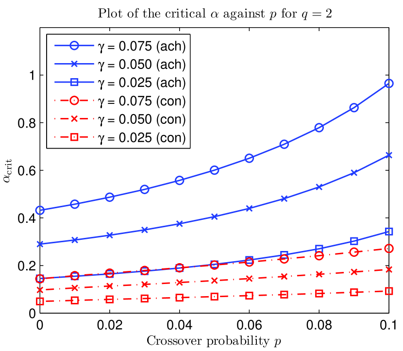
Figure 1: Plot of $\alpha_{\mathrm{crit}}$ against $p$ for $q=2$. Both $\alpha_{\mathrm{crit}}$ for the converse (con) in (37) the achievability (ach) in (39) are shown. All $\alpha$’s below the converse curves are not achievable.

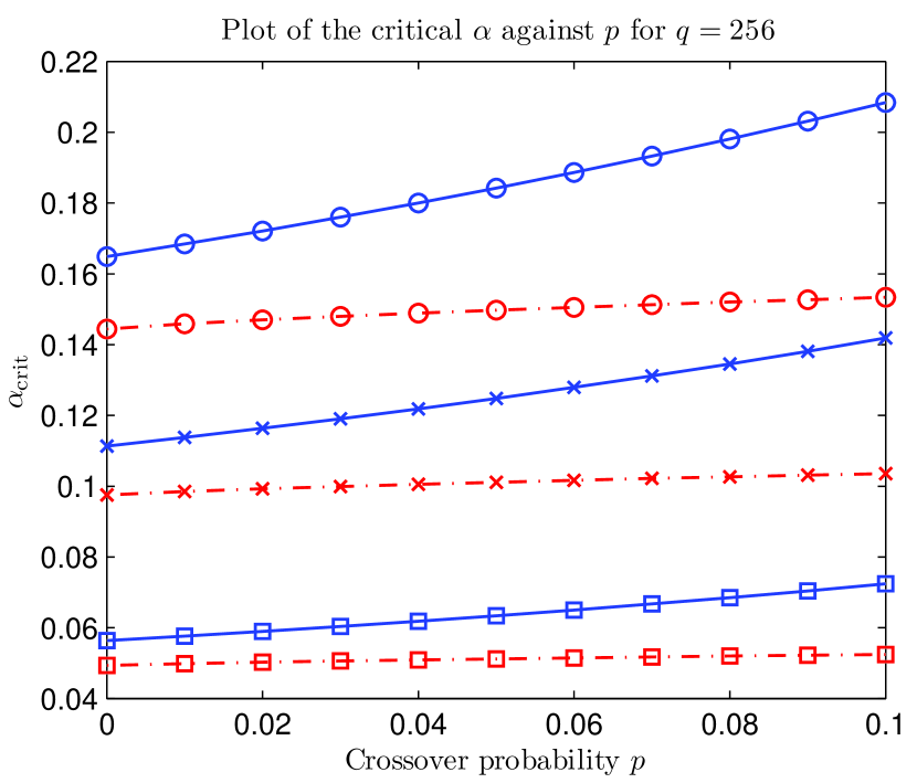
Figure 2: Plot of $\alpha_{\mathrm{crit}}$ against $p$ for $q=256$. See Fig. 1 for the legend.

From Fig. 1, we observe that the noise results in a significant increase in the critical value of the scaling parameter $\alpha$ when $q=2$. We see that for a rank-dimension ratio of $\gamma=0.05$ and with a crossover probability of $p=0.02$, the critical scaling parameter is $\alpha_{\mathrm{crit}}\approx 0.32$. Contrast this to the noiseless case (Proposition 3) and the converse result for the noisy case (Corollary 9) which stipulate that the critical scaling parameters are $2\gamma(1-\gamma/2)\approx 0.098$ and $2\gamma(1-\gamma/2)/(1-H_{2}(p))\approx 0.114$ respectively. Hence, we incur roughly a threefold increase in the number of measurements to tolerate a noise level of $p=2\%$. This phenomenon is due to our incognizance of the locations of the non-zero elements of $\mathbsf{w}$ (and hence knowledge of which measurements $\mathsf{y}_{a}$ are reliable). In contrast to the reals, in the finite field setting, there is no notion of the “size” of the noise (per measurement). Hence, estimation performance in the presence of noise does not degrade as gracefully as in the reals (cf. [6, Theorem 1.2]). However, when the field size is large (more likened to the reals), the degradation is not as severe. This is depicted in Fig. 2. Under the same settings as above, $\alpha_{\mathrm{crit}}\approx 0.114$, which is not too far from the converse ($2\gamma(1-\gamma/2)/(1-H_{256}(p))\approx 0.099$).

As a final remark, we compare the decoders for the noisy model in (34) and that in [31]. In [31], the authors considered the (analog of) following decoder (for tensors):

$$\operatorname{minimize}\quad\,\,\operatorname{rank}(\tilde{\mathbf{X}})$$

$$\operatorname{subject\,\,to}\quad\|\,\mathbsf{y}_{\tilde{\mathbf{X}}}-\mathbsf{y}\,\|_{0}\leq\tau,$$ (40)

where $\mathbsf{y}_{\tilde{\mathbf{X}}}:=[\langle{\mathbsf{H}_{1}},{\tilde{\mathbf{X}}}\rangle\,\ldots\,\langle{\mathbsf{H}_{k}},{\tilde{\mathbf{X}}}\rangle]^{T}$ and $\mathbsf{y}=\mathsf{y}^{k}$ is the noisy observation vector in (3). However, the threshold $\tau$ that constrains the Hamming distance between $\mathbsf{y}_{\tilde{\mathbf{X}}}$ and $\mathbsf{y}$ is not straightforward to choose. Our decoder, in contrast, is parameter-free because the regularization constant $\lambda$ in (34) can be chosen to be $1/n$, independent of all other parameters. In addition, Fig. 3 shows that at high $q$, our decoder and analysis result in a better (smaller) $\alpha_{\mathrm{crit}}$ than that in [31]. Our decoding scheme gives a bound that is closer to the converse at high $q$ while the decoding scheme in [31] is farther. The slight disadvantage of our decoder is that the number of measurements in (39) cannot be expressed in closed-form.

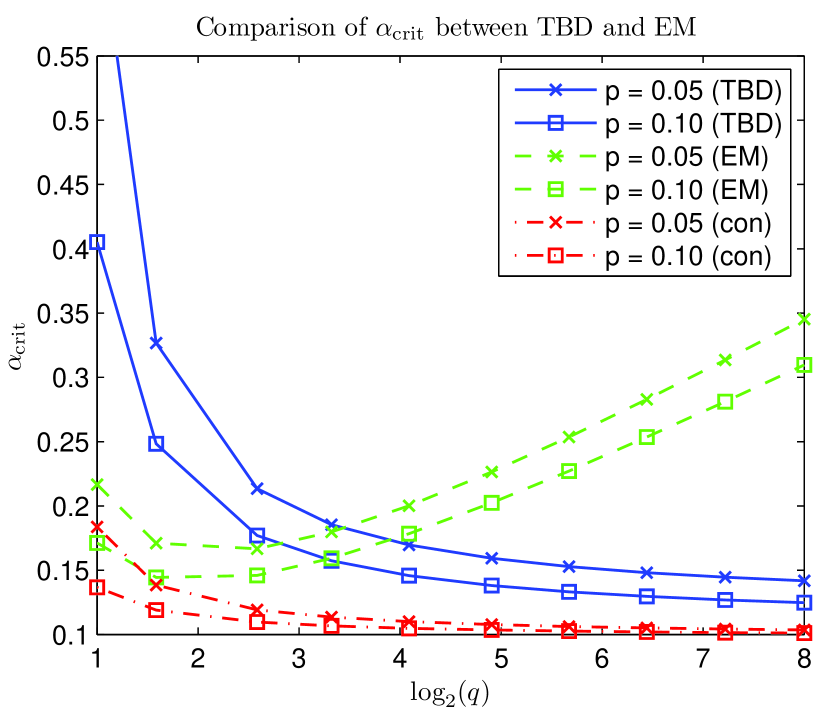
Figure 3: Plot of $\alpha_{\mathrm{crit}}$ against $\log_{2}(q)$ for our work (TBD Corollary 10), the converse in Corollary 9 and Emad and Milenkovic (EM) [31].

VI Sparse Random Sensing Matrices

In the previous two sections, we focused exclusively on the case where the elements of the sensing matrices $\mathbsf{H}_{a},a\in[k],$ are drawn uniformly from $\mathbb{F}_{q}$. However, there is substantial motivation to consider other ensembles of sensing matrices. For example, in low-density parity-check (LDPC) codes, the parity-check matrix (analogous to the set of $\mathbsf{H}_{a}$ matrices) is sparse. The sparsity aids in decoding via the sum-product algorithm [39] as the resulting Tanner (factor) graph is sparse [26]. In [32], the authors considered the case where the generator matrices are sparse and random but their setting is restricted to the BSC and BEC channel models.

In this section, we revisit the noiseless model in (2) and analyze the scenario where the sensing matrices are sparse on average. More precisely, each element of $\mathbsf{H}_{a},a\in[k],$ is assumed to be an i.i.d. random variable with associated pmf

$$P_{\mathsf{h}}(h;\delta,q):=\left\{\begin{array}[]{cc}1-\delta&h=0\\ \delta/(q-1)&h\in\mathbb{F}_{q}\setminus\{0\}\\ \end{array}\right..$$ (41)

Note that if $\delta$ is small, then the probability that an entry in $\mathbsf{H}_{a}$ is zero is close to unity. The problem of deriving a sufficient condition for reliable recovery is more challenging as compared to the equiprobable case since (18) no longer holds (compare to Lemma 21). Roughly speaking, the matrix $\mathbf{X}$ is not sensed as much as in the equiprobable case and the measurements $\mathsf{y}^{k}$ are not as informative because $\mathbsf{H}_{a},a\in[k]$, are sparse. In the rest of this section, we allow the sparsity factor $\delta$ to depend on $n$ but we do not make the dependence of $\delta$ on $n$ explicit for ease of exposition. The question we would like to answer is: How fast can $\delta$ decay with $n$ such that the min-rank decoder is still reliable for weak recovery?

Theorem 11 (Achievability under sparse measurement model).

Fix $\varepsilon>0$ and let $\delta$ be any sequence in $\Omega(\frac{\log n}{n})\cap o(1)$. Under the sparse measurement model as in (41), if the number of measurements $k$ satisfies (15) for all $n>N_{\varepsilon,\delta}$, then $\mathbb{P}(\mathcal{E}_{n})\to 0$ as $n\to\infty$.

The proof of Theorem 11, our main result, is detailed in Appendix E. It utilizes a “splitting” technique to partition the set of misleading matrices $\{\mathbf{Z}\neq\mathbf{X}:\operatorname{rank}(\mathbf{Z})\leq\operatorname{rank}(\mathbf{X})\}$ into those with low Hamming distance from $\mathbf{X}$ and those with high Hamming distance from $\mathbf{X}$.

Observe that the sparsity-factor $\delta$ is allowed to tend to zero albeit at a controlled rate of $\Omega(\frac{\log n}{n})$. Thus, each $\mathbsf{H}_{a}$ is allowed to have, on average, $\Omega(n\log n)$ non-zero entries (out of $n^{2}$ entries). The scaling rate is reminiscent of the number of trials required for success in the so-called coupon collector’s problem. Indeed, it seems plausible that we need at least one entry in each row and one entry in each column of $\mathbf{X}$ to be sensed (by a sensing matrix $\mathbsf{H}_{a}$) for the min-rank decoder to succeed. It can easily be seen that if $\delta=o(\frac{\log n}{n})$, there will be at least one row and one column in $\mathbsf{H}_{a}$ of zero Hamming weight w.h.p. Really surprisingly, the number of measurements required in the $\delta=\Omega(\frac{\log n}{n})$-sparse sensing case is exactly the same as in the case where the elements of $\mathbsf{H}_{a}$ are drawn uniformly at random from $\mathbb{F}_{q}$ in Proposition 3. In fact it also matches the information-theoretic lower bound in Proposition 2 and hence is asymptotically optimal. We will analyze this weak recovery sparse setting (and understand why it works) in greater detail by studying minimum distance properties of sparse parity-check rank-metric codes in Section VII-B. The sparse scenario may be extended to the noisy case by combining the proof techniques in Proposition 8 and Theorem 11.

There are two natural questions at this point: Firstly, can the reliability function be computed for the min-rank decoder assuming the sparse measurement model? The events $\mathcal{A}_{\mathbf{Z}}$, defined in (16), are no longer pairwise independent. Thus, it is not straightforward to compute $\mathbb{P}(\mathcal{A}_{\mathbf{Z}}\cap\mathcal{A}_{\mathbf{Z}^{\prime}})$ as in the proof of Proposition 4. Further, de Caen’s lower bound may not be tight as in the case where the entries of the sensing matrices are drawn uniformly at random from $\mathbb{F}_{q}$. Our bounding technique for Theorem 11 only ensures that

$$\limsup_{n\to\infty}\frac{1}{n\log n}\log_{q}\mathbb{P}(\mathcal{E}_{n})\leq-C$$ (42)

for some non-trivial $C\in(0,\infty)$. Thus, instead of having a speed of $n^{2}$ in the large-deviations upper bound, we have a speed of $n\log n$. This is because $\delta$ is allowed to decay to zero. Whether the speed $n\log n$ is optimal is open. Secondly, is $\delta=\Omega(\frac{\log n}{n})$ the best (smallest) possible sparsity factor? Is there a fundamental tradeoff between the sparsity factor $\delta$ and (a bound on) the number of measurements $k$? We leave these for further research.

VII Coding-Theoretic Interpretations and Minimum Rank Distance Properties

This section is devoted to understand the coding-theoretic interpretations and analogs of the rank minimization problem in (12). In particular, we would like to understand the geometry of the random linear rank-metric codes that underpin the optimization problem in (12) for both the equiprobable ensemble in (14) and the sparse ensemble in (41).

As mentioned in the Introduction, there is a natural correspondence between the rank minimization problem and rank-metric decoding [7, 8, 10, 9, 11, 12]. In the former, we solve a problem of the form (12). In the latter, the code $\mathscr{C}$ typically consists of length-$n$ vectors whose elements belong to the extension field $\mathbb{F}_{q^{n}}$ and these vectors in $\mathbb{F}_{q^{n}}^{n}$ a belong to the kernel of some linear operator $\mathbf{H}$. A particular vector codeword $\mathbf{c}\in\mathscr{C}$ is transmitted. The received word is $\mathbf{r}=\mathbf{c}+\mathbf{x},$ where $\mathbf{x}$ is assumed to be a low-rank “error” vector. (By rank of a vector we mean that there exists a fixed basis of $\mathbb{F}_{q^{n}}$ over $\mathbb{F}_{q}$ and the rank of a vector $\mathbf{a}\in\mathbb{F}_{q^{n}}^{n}$ is defined as the rank of the matrix $\mathbf{A}\in\mathbb{F}_{q}^{n\times n}$ whose elements are the coefficients of $\mathbf{a}$ in the basis. See [10, Sec. VI.A] for details of this isomorphic map.) The optimization problem for decoding $\mathbf{c}$ given $\mathbf{r}$ is then

$$\operatorname{minimize}\,\quad\operatorname{rank}(\mathbf{r}-\mathbf{c})$$

$$\operatorname{subject\,\,to}\quad\mathbf{c}\in\mathscr{C}$$ (43)

which is identical to the min-rank problem in (12) with the identification of the low error vector $\mathbf{x}\equiv\mathbf{r}-\mathbf{c}$. Note that the matrix version of the vector $\mathbf{r}$ (assuming a fixed basis), denoted as $\mathbf{R}$, satisfies the linear constraints in (2). Since the assignment $(\mathbf{A},\mathbf{B})\mapsto\operatorname{rank}(\mathbf{A}-\mathbf{B})$ is a metric on the space of matrices [10, Sec. II.B], the problem in (43) can be interpreted as a minimum (rank) distance decoder.

VII-A Distance Properties of Equiprobable Rank-Metric Codes

We formalize the notion of an equiprobable linear code and analyze its rank distance properties in this section. The results we derive here are the rank-metric analogs of the results in Barg and Forney [19] and will prove to be useful in shedding light on the geometry involved in the sufficient condition for recovering the unknown low-rank matrix $\mathbf{X}$ in Proposition 3.

Definition 3.

A rank-metric code is a non-empty subset of $\mathbb{F}_{q}^{n\times n}$ endowed with the the rank distance $(\mathbf{A},\mathbf{B})\mapsto\operatorname{rank}(\mathbf{A}-\mathbf{B})$.

Definition 4.

We say that $\mathscr{C}\subset\mathbb{F}_{q}^{n\times n}$ is an equiprobable linear rank-metric code if

$$\mathscr{C}:=\{\mathbf{C}\in\mathbb{F}_{q}^{n\times n}:\langle{\mathbf{C}},{\mathbsf{H}_{a}}\rangle=0,a\in[k]\}$$ (44)

where $\mathbsf{H}_{a},a\in[k]$ are random matrices where each entry is statistically independent of other entries and equiprobable in $\mathbb{F}_{q}$, i.e., with pmf given in (14). Each matrix $\mathbf{C}\in\mathscr{C}$ is called a codeword. Each matrix $\mathbsf{H}_{a}$ is said to be a parity-check matrix.

Recall that the inner product is defined as $\langle{\mathbf{C}},{\mathbsf{H}_{a}}\rangle=\mathrm{Tr}(\mathbf{C}\,\mathbsf{H}_{a}^{T})$. We reiterate that in the coding theory literature [7, 8, 10, 9, 11, 12], rank-metric codes usually consist of length-$n$ vectors $\mathbf{c}\in\mathscr{C}$ whose elements belong to the extension field $\mathbb{F}_{q^{n}}$. We refrain from adopting this approach here as we would like to make direct comparisons to the rank minimization problem, where the measurements are generated as in (2). Hence, the term codewords will always refer to matrices in $\mathscr{C}$.

Definition 5.

The number of codewords in the code $\mathscr{C}$ of rank $r$ ($r=0,1,\ldots,n$) is denoted as $\mathsf{N}_{\mathscr{C}}(r)$.

Note that $\mathsf{N}_{\mathscr{C}}(r)$ is a random variable since $\mathscr{C}\subset\mathbb{F}_{q}^{n\times n}$ is a random subspace. This quantity can also be expressed as

$$\mathsf{N}_{\mathscr{C}}(r):=\sum_{\mathbf{M}\in\mathbb{F}_{q}^{n\times n}:\operatorname{rank}(\mathbf{M})=r}\mathbb{I}\{\mathbf{M}\in\mathscr{C}\},$$ (45)

where $\mathbb{I}\{\mathbf{M}\in\mathscr{C}\}$ is the (indicator) random variable which takes on the value one if $\mathbf{M}\in\mathscr{C}$ and zero otherwise. Note that the matrix $\mathbf{M}$ is deterministic, while the code $\mathscr{C}$ is random. We remark that the decomposition of $\mathsf{N}_{\mathscr{C}}(r)$ in (45) is different from that in Barg and Forney [19, Eq. (2.3)] where the authors considered and analyzed the analog of the sum

$$\tilde{\mathsf{N}}_{\mathscr{C}}(r):=\sum_{j\in\{1,\ldots,|\mathscr{C}|\}\,:\,\mathbsf{C}_{j}\neq\mathbf{0}}\mathbb{I}\{\operatorname{rank}(\mathbsf{C}_{j})=r\},$$ (46)

where $j\in\{1,\ldots,|\mathscr{C}|\}$ indexes the (random) codewords in $\mathscr{C}$. Note that $\tilde{\mathsf{N}}_{\mathscr{C}}(r)={\mathsf{N}}_{\mathscr{C}}(r)$ for all $r\geq 1$ but they differ when $r=0$ ($\tilde{\mathsf{N}}_{\mathscr{C}}(0)=0$ while ${\mathsf{N}}_{\mathscr{C}}(0)=1$). It turns out that the sum in (45) is more amenable to analysis given that our parity-check (sensing) matrices $\mathbsf{H}_{a},a\in[k],$ are random (as in Gallager’s work in [20, Theorem 2.1]) whereas in [19, Sec. II.C], the generators are random. Recall the rank-dimension ratio $\gamma$ is the limit of the ratio $r/n$ as $n\to\infty$. Using (45), we can show the following:

Lemma 12 (Moments of $\mathsf{N}_{\mathscr{C}}(r)$).

For $r=0$, $\mathsf{N}_{\mathscr{C}}(r)=1$. For $1\leq r\leq n$, the mean of $\mathsf{N}_{\mathscr{C}}(r)$ satisfies

$$q^{-k+2rn-r^{2}-2r}\leq\mathbb{E}\mathsf{N}_{\mathscr{C}}(r)\leq 4q^{-k+2rn-r^{2}}.$$ (47)

Furthermore, the variance of $\mathsf{N}_{\mathscr{C}}(r)$ satisfies

$$\operatorname{var}(\mathsf{N}_{\mathscr{C}}(r)) \leq\mathbb{E}\mathsf{N}_{\mathscr{C}}(r).$$ (48)

The proof of Lemma 12 is provided in Appendix F. Observe from (47) that the average number of codewords with rank $r$, namely $\mathbb{E}\mathsf{N}_{\mathscr{C}}(r)$, is exponentially large (in $n^{2}$) if $k<(2-\varepsilon)\gamma(1-\gamma/2)n^{2}$ (compare to the converse in Proposition 2) and exponentially small if $k>(2+\varepsilon)\gamma(1-\gamma/2)n^{2}$ (compare to the achievability in Proposition 3). By Chebyshev’s inequality, an immediate corollary of Lemma 12 is the following:

Corollary 13 (Concentration of number of codewords of rank $r$).

Let $f_{n}$ be any sequence such that $\lim_{n\to\infty}f_{n}=\infty$. Then,

$$\lim_{n\to\infty}\mathbb{P}\left(|\mathsf{N}_{\mathscr{C}}(r)-\mathbb{E}\mathsf{N}_{\mathscr{C}}(r)|\geq f_{n}\sqrt{\mathbb{E}\mathsf{N}_{\mathscr{C}}(r)}\right)=0.$$ (49)

Thus, $\mathsf{N}_{\mathscr{C}}(r)$ concentrates to its mean in the sense of (49). A similar result for the random generator case was developed in [9, Corollary 1]. Also, our derivations based on Lemma 12 are cleaner and require fewer assumptions. We now define the notion of the minimum rank distance of a rank-metric code.

Definition 6.

The minimum rank distance of a rank-metric code $\mathscr{C}$ is defined as

$$\mathsf{d}_{\mathrm{R}}(\mathscr{C}):=\min_{\mathbf{C}_{1},\mathbf{C}_{2}\in\mathscr{C}:\mathbf{C}_{1}\neq\mathbf{C}_{2}}\operatorname{rank}(\mathbf{C}_{1}-\mathbf{C}_{2}).$$ (50)

By linearity of the code $\mathscr{C}$, it can be seen that the minimum rank distance in (50) can also be written as

$$\mathsf{d}_{\mathrm{R}}(\mathscr{C}):=\min_{\mathbf{C}\in\mathscr{C}:\mathbf{C}\neq\mathbf{0}}\operatorname{rank}(\mathbf{C}).$$ (51)

Thus, the minimum rank distance of a linear code is equal to the minimum rank over all non-zero matrix codewords.

Definition 7.

The relative minimum rank distance of a code $\mathscr{C}\subset\mathbb{F}_{q}^{n\times n}$ is defined as $\mathsf{d}_{\mathrm{R}}(\mathscr{C})/n$.

Note that the relative minimum rank distance is a random variable taking on values in the unit interval. In this section, we assume there exists some $\alpha\in(0,1)$ such that $k/n^{2}\to\alpha$ (cf. Section V-B). This is the scaling regime of interest.

Proposition 14 (Asymptotic linear independence).

Assume that each random matrix $\mathbsf{H}_{a}\in\mathbb{F}_{q}^{n\times n}$ consists of independent entries that are drawn according to the pmf in (41). Let $\mathsf{m}:=\dim(\mathrm{span}\{\operatorname{vec}(\mathbsf{H}_{1}),\ldots,\operatorname{vec}(\mathbsf{H}_{k})\})$. If $\delta\in\Omega(\frac{\log n}{n})$, then $\mathsf{m}/k\to 1$ almost surely (a.s.).

The proof of this proposition is a consequence of a result by Blömer et al. [42]. We provide the details in Appendix G.

We would now like to define the notion of the rate of a random code. Strictly speaking, since $\mathscr{C}$ is a random linear code, the rate of the code should be defined as the random variable $\tilde{\mathsf{R}}_{n}:=1-\mathsf{m}/n^{2}$. However, a consequence of Proposition 14 is that $\tilde{\mathsf{R}}_{n}/(1-k/n^{2})\to 1$ a.s. if $\delta\in\Omega(\frac{\log n}{n})$. Note that this prescribed rate of decay of $\delta$ subsumes the equiprobable model (of interest in this section) as a special case. (Take $\delta=(q-1)/q$ to be constant.) In light of Proposition 14, we adopt the following definition:

Definition 8.

The rate of the linear rank-metric code $\mathscr{C}$ [as in (44)] is defined as

$$R_{n}:=\frac{n^{2}-k}{n^{2}}=1-\frac{k}{n^{2}}.$$ (52)

The limit of $R_{n}$ in (52) is denoted as $R\in[0,1]$. Note also that $\tilde{\mathsf{R}}_{n}/R\to 1$ a.s.

Proposition 15 (Lower bound on relative minimum distance).

Fix $\varepsilon>0$. For any $R\in[0,1]$, the probability that the equiprobable linear code in (44) has relative minimum rank distance less than $1-\sqrt{R}-\varepsilon$ goes to zero as $n\to\infty$.

Proof.

Assume $\varepsilon\in(0,2(1-\gamma))$ and define the positive constant $\varepsilon^{\prime}:=2\varepsilon(1-\gamma)-\varepsilon^{2}$. Consider a sequence of ranks $r$ such that $r/n\to\gamma\leq 1-\sqrt{R}-\varepsilon$. Fix $\eta=\varepsilon^{\prime}/2>0$. Then, by Markov’s inequality and (47), we have

$$\mathbb{P}(\mathsf{N}_{\mathscr{C}}(r)\geq 1)\leq\mathbb{E}\mathsf{N}_{\mathscr{C}}(r)\leq 4q^{-n^{2}[\frac{k}{n^{2}}-2\gamma(1-\gamma/2)-\eta]},$$ (53)

for all $n>N_{\varepsilon^{\prime}}$. Since $\gamma\leq 1-\sqrt{R}-\varepsilon$, we may assert by invoking the definition of $R$ that $k\geq(2\gamma(1-\gamma/2)+\varepsilon^{\prime})n^{2}$. Hence, the exponent in square parentheses in (53) is no smaller than $\varepsilon^{\prime}/2$. This implies that $\mathbb{P}(\mathsf{N}_{\mathscr{C}}(r)\geq 1)\to 0$ or equivalently, $\mathbb{P}(\mathsf{N}_{\mathscr{C}}(r)=0)\to 1$. In other words, there are no matrices of rank $r$ in the equiprobable linear code $\mathscr{C}$ with probability at least $1-4q^{-\varepsilon^{\prime}n^{2}/2}$ for all $n>N_{\varepsilon^{\prime}}$. ∎

We now introduce some additional notation. We say that two positive sequences $\{a_{n}\}_{n\in\mathbb{N}}$ and $\{b_{n}\}_{n\in\mathbb{N}}$ are equal to second order in the exponent (denoted $a_{n}\stackrel{{\scriptstyle\,..}}{{=}}b_{n}$) if

$$\lim_{n\to\infty}\frac{1}{n^{2}}\log_{q}\frac{a_{n}}{b_{n}}=0.$$ (54)

Proposition 16 (Concentration of relative minimum distance).

Fix $\varepsilon>0$. For any $R\in[0,1]$, if $r$ is a sequence of ranks such that $r/n\to\gamma\geq 1-\sqrt{R}+\varepsilon$, then the probability that $\mathsf{N}_{\mathscr{C}}(r)\stackrel{{\scriptstyle\,..}}{{=}}q^{-k+2\gamma(1-\gamma/2)n^{2}}$ goes to one as $n\to\infty$.

Proof.

If the sequence of ranks $r$ is such that $r/n\to\gamma\geq 1-\sqrt{R}+\varepsilon$, then the average number of matrices in the code of rank $r$, namely $\mathbb{E}\mathsf{N}_{\mathscr{C}}(r)$, is exponentially large. By Markov’s inequality and the triangle inequality,

$$\mathbb{P}(|\mathsf{N}_{\mathscr{C}}(r)-\mathbb{E}\mathsf{N}_{\mathscr{C}}(r)|\geq t) \leq\frac{\mathbb{E}|\mathsf{N}_{\mathscr{C}}(r)-\mathbb{E}\mathsf{N}_{\mathscr{C}}(r)|\ }{t}$$

$$\leq\frac{2\mathbb{E}\mathsf{N}_{\mathscr{C}}(r)}{t}.$$ (55)

Choose $t:=q^{-k+(2\gamma(1-\gamma/2)+\eta)n^{2}+n}$, where $\eta$ is given in the proof of Proposition 15. Then, applying (47) to (VII-A) yields

$$\mathbb{P}(|\mathsf{N}_{\mathscr{C}}(r)-\mathbb{E}\mathsf{N}_{\mathscr{C}}(r)|\geq t)\leq 8q^{-n}\to 0.$$ (56)

Hence, $\mathsf{N}_{\mathscr{C}}(r)\in(\mathbb{E}\mathsf{N}_{\mathscr{C}}(r)-t,\mathbb{E}\mathsf{N}_{\mathscr{C}}(r)+t)$ with probability exceeding $1-8q^{-n}$. Furthermore, it is easy to verify that $\mathbb{E}\mathsf{N}_{\mathscr{C}}(r)\pm t\stackrel{{\scriptstyle\,..}}{{=}}q^{-k+2\gamma(1-\gamma/2)n^{2}}$, as desired.∎

Propositions 15 and 16 allow us to conclude that with probability approaching one (exponentially fast) as $n\to\infty$, the relative minimum rank distance of the equiprobable linear code in (44) is contained in the interval $(1-\sqrt{R}-\varepsilon,1-\sqrt{R}+\varepsilon)$ for all $R\in[0,1]$. The analog of the Gilbert-Varshamov (GV) distance [19, Sec. II.C] is thus

$$\gamma_{\mathrm{GV}}(R):=1-\sqrt{R}.$$ (57)

Indeed, by substituting the definition of $R$ into $\mathsf{N}_{\mathscr{C}}(r)$ in Proposition 16, we see that a typical (in the sense of [19]) equiprobable linear rank-metric code has distance distribution:

$$\mathsf{N}_{\mathrm{typ}}(r)\left\{\begin{array}[]{cc}\!\stackrel{{\scriptstyle\,..}}{{=}}\,q^{n^{2}[R-(1-\gamma)^{2}]}&\gamma\geq\gamma_{\mathrm{GV}}(R)+\varepsilon,\\ \!\!\!\!\!\!\!\!\!\!\!\!\!\!\!\!\!\!\!\!\!\!\!\!\!\!\!\!\!\!\!=\,0&\gamma\leq\gamma_{\mathrm{GV}}(R)-\varepsilon.\end{array}\right.$$ (58)

We again remark that Loidreau in [9, Sec. 5] also derived results for uniformly random linear codes in the rank-metric that are somewhat similar to Propositions 15 and 16. However, our derivations are more straightforward and require fewer assumptions. As mentioned above, we assume that the parity-check matrices $\mathbsf{H}_{a},a\in[k],$ are random (akin to [20, Theorem 2.1]), while the assumption in [9, Sec. 5] is that the generators are random and linearly independent. Furthermore, to the best of our knowledge, there are no previous studies on the minimum distance properties for the sparse parity-check matrix setting. We do this in Section VII-B.

From the rank distance properties, we can re-derive the achievability (weak recovery) result in Proposition 3 by using the definition of $R$ and solving the following inequality for $k$:

$$1-\sqrt{R}-\varepsilon\geq\gamma.$$ (59)

This provides geometric intuition as to why the min-rank decoder succeeds on average; the typical relative minimum rank distance of the code should exceed the rank-dimension ratio for successful error correction. We derive a stronger condition (known as the strong recovery condition) in Section VII-C.

VII-B Distance Properties of Sparse Rank-Metric Codes

In this section, we derive the analog of Proposition 15 for the case where the code $\mathscr{C}$ is characterized by sparse sensing (or measurement or parity-check) matrices $\mathbsf{H}_{a},a\in[k]$.

Definition 9.

We say that $\mathscr{C}$ is a $\delta$-sparse linear rank-metric code if $\mathscr{C}$ is as in (44) and where $\mathbsf{H}_{a},a\in[k]$ are random matrices where each entry is statistically independent and drawn from the pmf $P_{\mathsf{h}}(\,\cdot\,;\delta,q)$ defined in (41).

To analyze the number of matrices of rank $r$ in this random ensemble $\mathsf{N}_{\mathscr{C}}(r)$, we partition the sum in (45) into subsets of matrices based on their Hamming weight, i.e.,

$$\mathsf{N}_{\mathscr{C}}(r)=\sum_{d=0}^{n^{2}}\,\,\sum_{\mathbf{M}\in\mathbb{F}_{q}^{n\times n}:\operatorname{rank}(\mathbf{M})=r,\|\mathbf{M}\|_{0}=d}\mathbb{I}\{\mathbf{M}\in\mathscr{C}\}.$$ (60)

Define $\theta(d;\delta,q,k):=[q^{-1}+(1-q^{-1})(1-\delta/(1-q^{-1}))^{d}]^{k}$. As shown in Lemma 21 in Appendix E, this is the probability that a non-zero matrix $\mathbf{M}$ of Hamming weight $d$ belongs to the $\delta$-sparse code $\mathscr{C}$. We can demonstrate the following important bound for the $\delta$-sparse linear rank-metric code:

Lemma 17 (Mean of $\mathsf{N}_{\mathscr{C}}(r)$ for sparse codes).

For $r=0$, $\mathsf{N}_{\mathscr{C}}(r)=1$. If $1\leq r\leq n$ and $\eta>0$,

$$\mathbb{E}\mathsf{N}_{\mathscr{C}}(r) \leq 2^{n^{2}H_{2}(\beta)}(q-1)^{\beta n^{2}}(1-\delta)^{k}+$$

$$\,\,\,+4n^{2}q^{n^{2}\left[2\gamma(1-\gamma/2)+\eta+\frac{1}{n^{2}}\log_{q}\theta(\lceil{\beta n^{2}}\rceil;\,\delta,q,k)\right]},$$ (61)

for all $\beta\in[0,1/2]$ and all $n\geq N_{\eta}$.

By using the sum in (60), one sees that this lemma can be justified in exactly the same way as Theorem 11 (See steps leading to (83) and (84) in Appendix E). Hence, we omit its proof. Lemma 17 allows us to find a tight upper bound on the expectation of $\mathsf{N}_{\mathscr{C}}(r)$ for the sparse linear rank-metric code by optimizing over the free parameter $\beta\in[0,1/2]$. It turns out $\beta=\Theta(\frac{\delta}{\log n})$ is optimum. In analogy to Proposition 15 for the equiprobable linear rank-metric code, we can demonstrate the following for the sparse linear rank-metric code.

Proposition 18 (Lower bound on relative minimum distance for sparse codes).

Fix $\varepsilon>0$ assume that $\delta=\Omega(\frac{\log n}{n})\cap o(1)$. For any $R\in[0,1]$, the probability that the sparse linear code has relative minimum distance less than $1-\sqrt{R}-\varepsilon$ goes to zero as $n\to\infty$.

Proof.

The condition on the minimum distance implies that $k>(2+\tilde{\varepsilon})\gamma(1-\gamma/2)n^{2}$ for some $\tilde{\varepsilon}>0$ (for sufficiently small $\varepsilon$). See detailed argument in proof of Proposition 15. This implies from Theorem 11, Lemma 17 and Markov’s inequality that $\mathbb{P}(\mathsf{N}_{\mathscr{C}}(r)\geq 1)\to 0$.∎

Proposition 18 asserts that the relative minimum rank distance of a $\delta=\Omega(\frac{\log n}{n})$-sparse linear rank-metric code is at least $1-\sqrt{R}-\varepsilon$ w.h.p. Remarkably, this property is exactly the same as that of a (dense) linear code (cf. Proposition 15) in which the entries in the parity-check matrices $\mathbsf{H}_{a}$ are statistically independent and equiprobable in $\mathbb{F}_{q}$. The fact that the (lower bounds on the) minimum distances of both ensembles of codes coincide explains why the min-rank decoder matches the information-theoretic lower bound (Proposition 2) in the sparse setting (Theorem 11) just as in the dense one (Proposition 3). Note that only an upper bound of $\mathbb{E}\mathsf{N}_{\mathscr{C}}(r)$ as in (61) is required to make this claim.

VII-C Strong Recovery

We now utilize the insights gleaned from this section to derive results for strong recovery (See Section II-D and also [27, Sec. 2] for definitions) of low-rank matrices from linear measurements. Recall that in strong recovery, we are interested in recovering all matrices whose ranks are no larger than $r$. We contrast this to weak recovery where a matrix $\mathbf{X}$ (of low rank) is fixed and we ask how many random measurements are needed to estimate $\mathbf{X}$ reliably.

Proposition 19 (Strong recovery for uniform measurement model).

Fix $\varepsilon>0$. Under the uniform measurement model, the min-rank decoder recovers all matrices of rank less than or equal to $r$ with probability approaching one as $n\to\infty$ if

$$k>(4+\varepsilon)\gamma(1-\gamma)n^{2}.$$ (62)

We contrast this to the weak achievability result (Proposition 3) in which $\mathbf{X}$ with $\operatorname{rank}(\mathbf{X})\leq r$ was fixed and we showed that if $k>(2+\varepsilon)\gamma(1-\gamma/2)n^{2}$, the min-rank decoder recovers $\mathbf{X}$ w.h.p. Thus, Proposition 19 says that if $\gamma$ is small, roughly twice as many measurements are needed for strong recovery vis-à-vis weak recovery. These fundamental limits (and the increase in a factor of 2 for strong recovery) are exactly analogous those developed by Draper and Malekpour in [29] in the context of compressed sensing over finite fields and Eldar et al. [27] for the problem of rank minimization over the reals. Given our derivations in the preceding subsections, the proof of this result is straightforward.

Proof.

We showed in Proposition 15 that with probability approaching one (exponentially fast), the relative minimum distance of $\mathscr{C}$ is no smaller than $1-\sqrt{R}-\tilde{\varepsilon}$ for any $\tilde{\varepsilon}>0$. As such to guarantee strong recovery, we need the decoding regions (associated to each codeword in $\mathscr{C}$) to be disjoint. In other words, the rank distance between any two distinct codewords $\mathbf{C}_{1},\mathbf{C}_{2}\in\mathscr{C}$ must exceed $2r$. See Fig. 4 for an illustration. In terms of the relative minimum rank distance $1-\sqrt{R}-\tilde{\varepsilon}$, this requirement translates to

$$1-\sqrt{R}-\tilde{\varepsilon}\geq 2\gamma.$$ (63)

Rearranging this inequality as and using the definition of $R$ [limit of $R_{n}$ in (52)] as we did in Proposition 15 yields the required number of measurements prescribed. ∎

In analogy to Proposition 19, we can show the following for the sparse model.

Proposition 20 (Strong recovery for sparse measurement model).

Fix $\varepsilon>0$. Under the $\delta=\Omega(\frac{\log n}{n})$-sparse measurement model, the min-rank decoder recovers all matrices of rank less than or equal to $r$ with probability approaching one as $n\to\infty$ if (62) holds.

Proof.

The proof uses Proposition 18 and follows along the exact same lines as that of Proposition 19. ∎

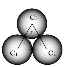
Figure 4: For strong recovery, the decoding regions associated to each codeword $\mathbf{C}\in\mathscr{C}$ have to be disjoint, resulting in the criterion in (63).

VIII Reduction in the Complexity of the Min-Rank Decoder

In this section, we devise a procedure to reduce the complexity for min-rank decoding (vis-à-vis exhaustive search). This procedure is inspired by techniques in the cryptography literature [43, 44]. We adapt the techniques for our problem which is somewhat different. As we mentioned in Section VII, the codewords in this paper are matrices rather than vectors whose elements belong to an extension field [43, 44].

Recall that in min-rank decoding (12), we search for a matrix $\mathbf{X}\in\mathbb{F}_{q}^{N\times n}$ of minimum rank that satisfies the linear constraints. In this section, for clarity of exposition, we differentiate between the number of rows ($N$) and the number of columns ($n$) in $\mathbf{X}$. The vector $\mathsf{y}^{k}$ is known as the syndrome.

We first suppose that the minimum rank in (12) is known to be equal to some integer $r\leq\min\{N,n\}$. Since our proposed algorithm requires exponentially many elementary operations (addition and multiplication) in $\mathbb{F}_{q}$, this assumption does not affect the time complexity significantly. Then the problem in (12) reduces to a satisfiability problem: Given an integer $r$, a collection of parity-check matrices $\mathbsf{H}_{a},a\in[k]$ and a syndrome vector $\mathsf{y}^{k}$, find (if possible) a matrix $\mathbf{X}\in\mathbb{F}_{q}^{N\times n}$ of rank exactly equal to $r$ that satisfies the linear constraints in (12). Note that the constrains in (12) are equivalent to $\langle{\operatorname{vec}(\mathbsf{H}_{a})},{\operatorname{vec}(\mathbf{X})}\rangle=\mathsf{y}_{a},a\in[k]$.

We first claim that we can, without loss of generality, assume that $\mathsf{y}^{k}=0^{k}$, i.e, the constraints in (12) read

$$\langle\mathbsf{H}_{a},\mathbf{X}\rangle=0,\quad a\in[k].$$ (64)

We justify this claim as follows: Consider the new syndrome-augmented vectors $[\operatorname{vec}(\mathbsf{H}_{a});\mathsf{y}_{a}]^{T}\in\mathbb{F}_{q}^{Nn+1}$ for every $a\in[k]$. Then, every solution $\operatorname{vec}(\mathbf{X}^{\prime})$ of the system of equations

$$\langle{[\operatorname{vec}(\mathbsf{H}_{a});\mathsf{y}_{a}]},{\operatorname{vec}(\mathbf{X}^{\prime})}\rangle=0,\quad a\in[k]$$ (65)

can be partitioned into two parts, $\operatorname{vec}(\mathbf{X}^{\prime})=[\operatorname{vec}(\mathbf{X}_{1});x_{2}]$ where $\operatorname{vec}(\mathbf{X}_{1})\in\mathbb{F}_{q}^{Nn}$ and $x_{2}\in\mathbb{F}_{q}$. Thus, every solution of (65) satisfies one of two conditions:

• $x_{2}=0$. In this case $\mathbf{X}_{1}$ is a solution to the linear equations in (12).

• $x_{2}\neq 0$. In this case $\mathbf{X}_{1}$ solves $\langle\mathbsf{H}_{a},\mathbf{X}_{1}\rangle=x_{2}\mathsf{y}_{a}$. Thus, $x_{2}^{-1}\mathbf{X}_{1}$ solves (12).

This is also known as coset decoding. Now, observe that since it is known that $\mathbf{X}$ has rank equal to $r$ (which is assumed known), it can be written as

$$\mathbf{X}=\sum_{l=1}^{r}\mathbf{u}_{l}\mathbf{v}_{l}^{T}=\mathbf{U}\mathbf{V}^{T}$$ (66)

where each of the vectors $\mathbf{u}_{l}\in\mathbb{F}_{q}^{N}$ and $\mathbf{v}_{l}\in\mathbb{F}_{q}^{n}$. The matrices $\mathbf{U}\in\mathbb{F}_{q}^{N\times r}$ and $\mathbf{V}\in\mathbb{F}_{q}^{n\times r}$ are of (full) rank $r$ and are referred to as the basis matrix and the coefficient matrix respectively. The linear system of equations in (64) can be expanded as

$$\sum_{l=1}^{r}\,\sum_{i=1}^{N}\,\sum_{j=1}^{n}\,[\mathbsf{H}_{a}]_{i,j}\,u_{l,i}\,v_{l,j}=0,\qquad a\in[k]$$ (67)

where $\mathbf{u}_{l}=[u_{l,1},\ldots,u_{l,N}]^{T}$ and $\mathbf{v}_{l}=[v_{l,1},\ldots,v_{l,n}]^{T}$. Thus, we need to solve a system of quadratic equations in the basis elements $u_{l,i}$ and the coefficients $v_{l,j}$.

VIII-A Naïve Implementation

A naïve way to find a consistent $\mathbf{U}$ and $\mathbf{V}$ for (67) is to employ the following algorithm:

1. Start with $r=1$.

2. Enumerate all bases $\mathbf{U}=\{u_{l,i}:i\in[N],l\in[r]\}$.

3. For each basis, solve (if possible) the resulting linear system of equations in $\mathbf{V}=\{v_{l,j}:j\in[n],l\in[r]\}$.

4. If a consistent set of coefficients $\mathbf{V}$ exists (i.e., (67) is satisfied), terminate and set $\mathbf{X}=\mathbf{U}\mathbf{V}^{T}$. Else increment $r\leftarrow r+1$ and go to step 2.

The second step can be solved easily if the number of equations is less than or equal to the number of unknowns, i.e., if $nr\geq k$. However, this is usually not the case since for successful recovery, $k$ has to satisfy (15) so, in general, there are more equations (linear constraints) than unknowns. We attempt to solve for (if possible) a consistent $\mathbf{V}$, otherwise we increment the guessed rank $r$. The computational complexity of this naïve approach (assuming $r$ is known and so no iterations over $r$ are needed) is $O((nr)^{3}q^{Nr})$ since there are $q^{Nr}$ distinct bases and solving the linear system via Gaussian elimination requires at most $O((nr)^{3})$ operations in $\mathbb{F}_{q}$.

VIII-B Simple Observations to Reduce the Search for the Basis $\mathbf{U}$

We now use ideas from [43, 44] and make two simple observations to dramatically reduce the search for the basis in step 2 of the above naïve implementation.

Observation (A): Note that if $\tilde{\mathbf{X}}$ solves (64), so does $\rho\tilde{\mathbf{X}}$ for any $\rho\in\mathbb{F}_{q}$. Hence, without loss of generality, we may assume that the we can scale the (1,1) element of $\mathbf{U}$ to be equal to 1. The number of bases we need to enumerate may thus be reduced by a factor of $q$.

Observation (B): Note that the decomposition $\mathbf{X}=\mathbf{U}\mathbf{V}^{T}$ is not unique. Indeed if $\mathbf{X}=\mathbf{U}\mathbf{V}^{T}$, we may also decompose $\mathbf{X}$ as $\mathbf{X}=\tilde{\mathbf{U}}\tilde{\mathbf{V}}^{T}$, where $\tilde{\mathbf{U}}=\mathbf{U}\mathbf{T}$ and $\tilde{\mathbf{V}}=\mathbf{V}\mathbf{T}^{-T}$ and $\mathbf{T}$ is any invertible $r\times r$ matrix over $\mathbb{F}_{q}$. We say that two bases $\mathbf{U},\tilde{\mathbf{U}}$ are equivalent, denoted $\mathbf{U}\sim\tilde{\mathbf{U}}$, if there exists an invertible matrix $\mathbf{T}$ such that $\mathbf{U}=\tilde{\mathbf{U}}\mathbf{T}$. The equivalence relation $\sim$ induces a partition of the set of $\mathbb{F}_{q}^{N\times r}$ matrices.

Let $[\mathbf{U}]:=\{\tilde{\mathbf{U}}\in\mathbb{F}_{q}^{N\times r}:\tilde{\mathbf{U}}\sim\mathbf{U}\}$ be the equivalence class of matrices containing the matrix $\mathbf{U}$. From the preceding discussion on the indeterminacies in the decomposition of the low rank matrix $\mathbf{X}$, we observe that the complexity involved in the enumeration of all $\mathbb{F}_{q}^{N\times r}$ matrices in step 2 in the naïve implementation can be reduced by only enumerating the different equivalence classes induced by $\sim$. More precisely, we find (if possible) coefficients $\mathbf{V}$ for a basis $\mathbf{U}$ from each equivalence class, e.g., $\mathbf{U}_{1}\in[\mathbf{U}_{1}],\ldots,\mathbf{U}_{m}\in[\mathbf{U}_{m}]$. Note that the number of equivalence classes (by Lagrange’s theorem) is

$$m=\frac{q^{Nr}}{\Phi_{q}(r,r)}\leq 4q^{r(N-r)},$$ (68)

where recall from Section II-E that $\Phi_{q}(r,r)$ is the number of non-singular matrices in $\mathbb{F}_{q}^{r\times r}$. The inequality arises from the fact that $\Phi_{q}(r,r)\geq\frac{1}{4}q^{r^{2}}$, a simple consequence of [43, Cor. 4]. Algorithmically, we can enumerate the equivalence classes by first considering all matrices of the form

$$\mathbf{U}=\begin{bmatrix}\mathbf{I}_{r\times r}\\ \mathbf{Q}\end{bmatrix},$$ (69)

where $\mathbf{I}_{r\times r}$ is the identity matrix of size $r$, and $\mathbf{Q}$ takes on all possible values in $\mathbb{F}_{q}^{(N-r)\times r}$. Note that if $\mathbf{Q}$ and $\tilde{\mathbf{Q}}$ are distinct, the corresponding $\mathbf{U}=[\mathbf{I};\mathbf{Q}^{T}]^{T}$ and $\tilde{\mathbf{U}}=[\mathbf{I};\tilde{\mathbf{Q}}^{T}]^{T}$ belong to different equivalence classes. However, the top $r$ rows of $\mathbf{U}$ may not be linearly independent so we have yet to consider all equivalence classes. Hence, we subsequently permute the rows of each previously considered $\mathbf{U}$ to ensure every equivalence class is considered.

From the considerations in (A) and (B), the computational complexity can be reduced from $O((nr)^{3}q^{Nr})$ to $O((nr)^{3}q^{r(N-r)-1})$. By further noting that there is symmetry between the basis matrix $\mathbf{U}$ and the coefficient matrix $\mathbf{V}$, we see that the resulting computational complexity is $O((\max\{n,N\}r)^{3}q^{r(\min\{n,N\}-r)-1})$. Finally, to incorporate the fact that $r$ is unknown, we start the procedure assuming $r=1$, proceed to $r\leftarrow r+1$ if there does not exist a consistent solution and so on, until a consistent $(\mathbf{U},\mathbf{V})$ pair is found. The resulting computational complexity is thus $O(r(\max\{n,N\}r)^{3}q^{r(\min\{n,N\}-r)-1}).$

IX Discussion and Conclusion

In this section, we elaborate on connections of our work to the related works mentioned the introduction and in Tables I and II. We will also conclude the paper by summarizing our main contributions and suggesting avenues for future research.

IX-A Comparison to existing coding-theoretic techniques for rank minimization over finite fields

In general, solving the min-rank decoding problem (43) is intractable (NP-hard). However, it is known that if the linear operator $\mathbf{H}$ (in (4) characterizing the code $\mathscr{C}$) admits a favorable algebraic structure, then one can estimate a sufficiently low-rank (vector with elements in the extension field $\mathbb{F}_{q^{n}}$ or matrix with elements in $\mathbb{F}_{q}$) $\mathbf{x}$ and thus the codeword $\mathbf{c}$ from the received word $\mathbf{r}$ efficiently (i.e., in polynomial time). For instance, the class of Gabidulin codes [7, 8], which are rank-metric analogs of Reed-Solomon codes, not only achieves the Singleton bound and thus has maximum rank distance (MRD), but decoding can be achieved using a modified form of the Berlekamp-Massey algorithm (See [45] for example). However, the algebraic structure of the codes (and in particular the mutual dependence between the equivalent $\mathbsf{H}_{a}$ matrices) does not permit the line of analysis we adopted. Thus it is unclear how many linear measurements would be required in order to guarantee recovery using the suggested code structure. Silva, Kschischang and Kötter [10] extended the Berlekamp-Massey-based algorithm to handle errors and erasures for the purpose of error control in linear random network coding. In both these cases, the underlying error matrix is assumed to be deterministic and the algebraic structure on the parity check matrix permitted efficient decoding based on error locators.

In another related work, Montanari and Urbanke [11] assumed that the error matrix $\mathbsf{X}$ is drawn uniformly at random from all matrices of known rank $r$. The authors then constructed a sparse parity check code (based on a sparse factor graph). Using an “error-trapping” strategy by constraining codewords to have rows that are have zero Hamming weight without any loss of rate, they first learned the rowspace of $\mathbsf{X}$ before adopting a (subspace) message passing strategy to complete the reconstruction. However, the dependence across rows of the parity check matrix (caused by lifting) violates the independence assumptions needed for our analyses to hold. The ideas in [11] were subsequently extended by Silva, Kschischang and Kötter [18] where the authors computed the information capacity of various (additive and/or multiplicative) matrix-valued channels over finite fields. They also devised “error-trapping” codes to achieve capacity. However, unlike this work, it is assumed in [18] that the underlying low-rank error matrix is chosen uniformly. As such, their guarantees do not apply to so-called crisscross error patterns [17, 45] (see Fig. 5), which are of interest in data storage applications.

Figure 5: Probabilistic crisscross error patterns [17]: The figure shows an error matrix $\mathbf{X}$. The non-zero values (indicated as black dots) are restricted to two columns and one row. Thus, the rank of the error matrix $\mathbf{X}$ is at most three.

Our work in this paper is focused primarily on understanding the fundamental limits of rank-metric codes that are random. More precisely, the codes are characterized by either dense or sparse sensing (parity-check) matrices. This is in contrast to the literature on rank-metric codes (except [9, Sec. 5]), in which deterministic constructions predominate. The codes presented in Section VII are random. However, in analogy to the random coding argument for channel coding [35, Sec. 7.7], if the ensemble of random codes has low average error probability, there exists a deterministic code that has low error probability. In addition, the strong recovery results in Section VII-C allow us to conclude that our analyses apply to all low-rank matrices $\mathbf{X}$ in both equiprobable and sparse settings. This completes all remaining entries in Table II.

Yet another line of research on rank minimization over finite fields (in particular over $\mathbb{F}_{2}$) has been conducted by the combinatorial optimization and graph theory communities. In [33, Sec. 6] and [46, Sec. 1] for example, it was demonstrated that if the code (or set of linear constraints) is characterized by a perfect graph, then the rank minimization problem can be solved exactly and in polynomial time by the ellipsoid method (since the problem can be stated as a semidefinite program). In fact, the rank minimization problem is also intimately related to Lovász’s $\theta$ function [47, Theorem 4], which characterizes the Shannon capacity of a graph.

IX-B Conclusion and Future Directions

In this paper, we derive information-theoretic limits for recovering a low-rank matrix with elements over a finite field given noiseless or noisy linear measurements. We show that even if the random sensing (or parity-check) matrices are very sparse, decoding can be done with exactly the same number of measurements as when the sensing matrices are dense. We then adopt a coding-theoretic approach and derived minimum rank distance properties of sparse random rank-metric codes. These results provide geometric insights as to how and why decoding succeeds when sufficiently many measurements are available. The work herein could potentially lead to the design of low-complexity sparse codes for rank-metric channels.

It is also of interest to analyze whether the sparsity factor of $\Theta(\frac{\log n}{n})$ is the smallest possible and whether there is a fundamental tradeoff between this sparsity factor and the number of measurements required for reliable recovery of the low-rank matrix. Additionally, in many of the applications that motivate this problem, the sensing matrices fixed by the application and will not be random; take for example deterministic parity-check matrices that might define a rank-metric code. In rank minimization in the real field there are properties about the sensing matrices, and about the underlying matrix being estimated, that can be checked (for example the restricted isometry property [6, Eq. (1)], or random point sampling joint with incoherence of the low-rank matrix) that, if they are satisfied, guarantee that the true matrix of interest can be recovered using convex programming. It is of interest to identify an analog in the finite field, that is, a necessary (or sufficient) condition on the sensing matrices and the underlying matrix such that recovery is guaranteed. We would like to develop tractable algorithms along the lines of those in Table I or in the work by Baron et al. [26] to solve the min-rank optimization problem approximately for particular classes of sensing matrices such as the sparse random ensemble.

Finally, Dimakis and Vontobel [48] make an intriguing connection between linear programming (LP) decoding for channel coding and LP decoding for compressed sensing. They reach known compressed sensing results via a new path – channel coding. Analogously, we wonder whether known rank minimization results can be derived using rank-metric coding tools, thereby providing novel interpretations. And just as in [48], the reverse direction is also open. That is, whether the growing literature and understanding of rank minimization problems could be leveraged to design more tractable and interesting decoding approaches for rank-metric codes.

Acknowledgements

We would like to thank Associate Editor Erdal Arıkan and the reviewers for their suggestions to improve the paper and to acknowledge discussions with Ron Roth, Natalia Silberstein and especially Danilo Silva, who made the insightful points in Section IV-B1 [38]. We would also like to thank Ying Liu and Huili Guo for detailed comments and help in generating Fig. 4 respectively.

Appendix A Proof of Lemma 6

Proof.

It suffices to show that the conditional probability $\mathbb{P}(\mathcal{A}_{\mathbf{Z}^{\prime}}|\mathcal{A}_{\mathbf{Z}})=\mathbb{P}(\mathcal{A}_{\mathbf{Z}^{\prime}})=q^{-k}$ for $\mathbf{Z}\neq\mathbf{Z}^{\prime}$. We define the non-zero matrices $\mathbf{M}:=\mathbf{X}-\mathbf{Z}$ and $\mathbf{M}^{\prime}:=\mathbf{X}-\mathbf{Z}^{\prime}$. Let $\mathcal{K}:=\operatorname{supp}(\mathbf{M}^{\prime}-\mathbf{M})$ and $\mathcal{L}:=\operatorname{supp}(\mathbf{M})$. The idea of the proof is to partition the joint support $\mathcal{K}\cup\mathcal{L}$ into disjoint sets. More precisely, consider

$$\mathbb{P}(\mathcal{A}_{\mathbf{Z}^{\prime}}|\mathcal{A}_{\mathbf{Z}}) \stackrel{{\scriptstyle(a)}}{{=}}\mathbb{P}(\langle{\mathbf{M}^{\prime}},{\mathbsf{H}_{1}}\rangle=0\,|\,\langle{\mathbf{M}},{\mathbsf{H}_{1}}\rangle=0)^{k}$$

$$\stackrel{{\scriptstyle(b)}}{{=}}\mathbb{P}(\langle{\mathbf{M}^{\prime}\!-\!\mathbf{M}},{\mathbsf{H}_{1}}\rangle\!=0\,|\,\langle{\mathbf{M}},{\mathbsf{H}_{1}}\rangle=0)^{k},$$ (70)

where $(a)$ is from the definition of $\mathcal{A}_{\mathbf{Z}}:=\{\langle{\mathbf{X}-\mathbf{Z}},{\mathbsf{H}_{a}}\rangle=0,\forall\,a\in[k]\}$ and the independence of the random matrices $\mathbsf{H}_{a},a\in[k]$ and $(b)$ by linearity. It suffices to show that the probability in (70) is $q^{-1}$. Indeed,

$$\mathbb{P}(\langle{\mathbf{M}^{\prime}-\mathbf{M}},{\mathbsf{H}_{1}}\rangle=0\,|\,\langle{\mathbf{M}},{\mathbsf{H}_{1}}\rangle=0)$$

$$\stackrel{{\scriptstyle(c)}}{{=}}\mathbb{P}\Big{(}\sum_{(i,j)\in\mathcal{K}}[\mathbf{M}^{\prime}-\mathbf{M}]_{i,j}[\mathbsf{H}_{1}]_{i,j}=0\,\Big{|}\,$$

$$\qquad\qquad\qquad\sum_{(i,j)\in\mathcal{L}}[\mathbf{M}]_{i,j}[\mathbsf{H}_{1}]_{i,j}=0\Big{)}$$

$$\stackrel{{\scriptstyle(d)}}{{=}}\mathbb{P}\Big{(}\sum_{(i,j)\in\mathcal{K}}[\mathbsf{H}_{1}]_{i,j}=0\,\Big{|}\,\sum_{(i,j)\in\mathcal{L}}[\mathbsf{H}_{1}]_{i,j}=0\Big{)},$$ (71)

where $(c)$ is from the definition of the inner product and the sets $\mathcal{K}$ and $\mathcal{L}$, $(d)$ from the fact that $[\mathbf{M}]_{i,j}[\mathbsf{H}_{1}]_{i,j}$ has the same distribution as $[\mathbsf{H}_{1}]_{i,j}$ since $[\mathbf{M}]_{i,j}\neq 0$ and $[\mathbsf{H}_{1}]_{i,j}$ is uniformly distributed in $\mathbb{F}_{q}$. Now, we split the sets $\mathcal{K}$ and $\mathcal{L}$ in (71) into two disjoint subsets each, obtaining

$$\mathbb{P}(\langle{\mathbf{M}^{\prime}-\mathbf{M}},{\mathbsf{H}_{1}}\rangle=0\,|\,\langle{\mathbf{M}},{\mathbsf{H}_{1}}\rangle=0)$$

$$=\mathbb{P}\Big{(}\sum_{(i,j)\in\mathcal{K}\setminus\mathcal{L}}[\mathbsf{H}_{1}]_{i,j}+\sum_{(i,j)\in\mathcal{L}\cap\mathcal{K}}[\mathbsf{H}_{1}]_{i,j}=0\,\Big{|}\,$$

$$\qquad\qquad\qquad\sum_{(i,j)\in\mathcal{L}\setminus\mathcal{K}}[\mathbsf{H}_{1}]_{i,j}+\sum_{(i,j)\in\mathcal{L}\cap\mathcal{K}}[\mathbsf{H}_{1}]_{i,j}=0\Big{)}$$

$$\stackrel{{\scriptstyle(e)}}{{=}}\mathbb{P}\Big{(}\sum_{(i,j)\in\mathcal{L}\setminus\mathcal{K}}[\mathbsf{H}_{1}]_{i,j}=\sum_{(i,j)\in\mathcal{K}\setminus\mathcal{L}}[\mathbsf{H}_{1}]_{i,j}\,\Big{|}\,$$

$$\qquad\qquad\sum_{(i,j)\in\mathcal{L}\setminus\mathcal{K}}[\mathbsf{H}_{1}]_{i,j}=-\sum_{(i,j)\in\mathcal{L}\cap\mathcal{K}}[\mathbsf{H}_{1}]_{i,j}\Big{)}\stackrel{{\scriptstyle(f)}}{{=}}q^{-1},$$

Equality $(e)$ is by using the condition $\sum_{(i,j)\in\mathcal{L}\setminus\mathcal{K}}[\mathbsf{H}_{1}]_{i,j}=-\sum_{(i,j)\in\mathcal{L}\cap\mathcal{K}}[\mathbsf{H}_{1}]_{i,j}$ and finally $(f)$ from the fact that the sets $\mathcal{K}\setminus\mathcal{L}$, $\mathcal{L}\setminus\mathcal{K}$ and $\mathcal{L}\cap\mathcal{K}$ are mutually disjoint so the probability is $q^{-1}$ by independence and uniformity of $[\mathbsf{H}_{1}]_{i,j},(i,j)\in[n]^{2}$.∎

Appendix B Proof of Proposition 8

Proof.

Recall the optimization problem for the noisy case in (34) where the optimization variables are $\tilde{\mathbf{X}}$ and $\tilde{\mathbf{w}}$. Let $\mathcal{S}^{\mathrm{noisy}}\subset\mathbb{F}_{q}^{n\times n}\times\mathbb{F}_{q}^{k}$ be the set of optimizers. In analogy to (13), we define the “noisy” error event

$$\mathcal{E}_{n}^{\mathrm{noisy}}\!\!:=\!\{|\mathcal{S}^{\mathrm{noisy}}|\!>\!1\}\cup(\{|\mathcal{S}^{\mathrm{noisy}}|\!=\!1\}\cap\{(\mathbsf{X}^{*},\mathbsf{w}^{*})\!\neq\!(\mathbf{X},\mathbf{w})\}).$$

Note that $(\mathcal{E}_{n}^{\mathrm{noisy}})^{c}$ occurs, both the matrix $\mathbf{X}$ and the noise vector $\mathbf{w}$ are recovered so, in fact, we are decoding two objects when we are only interested in $\mathbf{X}$. Clearly, $\mathcal{E}_{n}\subset\mathcal{E}_{n}^{\mathrm{noisy}}$ so it suffices to upper bound $\mathbb{P}(\mathcal{E}_{n}^{\mathrm{noisy}})$ to obtain an upper bound of $\mathbb{P}(\mathcal{E}_{n})$. For this purpose consider the event

$$\mathcal{A}_{\mathbf{Z},\mathbf{v}}^{\mathrm{noisy}}:=\{\langle{\mathbf{Z}},{\mathbsf{H}_{a}}\rangle=\langle\mathbf{X},\mathbsf{H}_{a}\rangle+v_{a},\forall\,a\in[k]\},$$ (72)

defined for each matrix-vector pair $(\mathbf{Z},\mathbf{v})\in\mathbb{F}_{q}^{n\times n}\times\mathbb{F}_{q}^{k}$ such that $\operatorname{rank}(\mathbf{Z})+\lambda\|\mathbf{v}\|_{0}\leq\operatorname{rank}(\mathbf{X})+\lambda\|\mathbf{w}\|_{0}$. The error event $\mathcal{E}_{n}^{\mathrm{noisy}}$ occurs if and only if there exists a pair $(\mathbf{Z},\mathbf{v})\neq(\mathbf{X},\mathbf{w})$ such that (i) $\operatorname{rank}(\mathbf{Z})+\lambda\|\mathbf{v}\|_{0}\leq\operatorname{rank}(\mathbf{X})+\lambda\|\mathbf{w}\|_{0}$ and (ii) the event $\mathcal{A}_{\mathbf{Z},\mathbf{v}}^{\mathrm{noisy}}$ occurs. By the union of events bound, the error probability can be bounded as:

$$\mathbb{P}(\mathcal{E}_{n}^{\mathrm{noisy}}) \leq\sum_{(\mathbf{Z},\mathbf{v}):\operatorname{rank}(\mathbf{Z})+\lambda\|\mathbf{v}\|_{0}\leq\operatorname{rank}(\mathbf{X})+\lambda\|\mathbf{w}\|_{0}}\mathbb{P}(\mathcal{A}_{\mathbf{Z},\mathbf{v}}^{\mathrm{noisy}})$$

$$\stackrel{{\scriptstyle(a)}}{{=}}\sum_{(\mathbf{Z},\mathbf{v}):\operatorname{rank}(\mathbf{Z})+\lambda\|\mathbf{v}\|_{0}\leq\operatorname{rank}(\mathbf{X})+\lambda\|\mathbf{w}\|_{0}}q^{-k}$$

$$\stackrel{{\scriptstyle(b)}}{{\leq}}q^{-k}|\mathcal{U}_{r,s}|,$$ (73)

where $(a)$ is from the same argument as the noiseless case [See (18)] and in $(b)$, we defined the set $\mathcal{U}_{r,s}:=\{(\mathbf{Z},\mathbf{v}):\operatorname{rank}(\mathbf{Z})+\lambda\|\mathbf{v}\|_{0}\leq\operatorname{rank}(\mathbf{X})+\lambda\|\mathbf{w}\|_{0}\}$, where the subscripts $r$ and $s$ index respectively the upper bound on the rank of $\mathbf{X}$ and sparsity of $\mathbf{w}$. Note that $s=\|\mathbf{w}\|_{0}=\lfloor{\sigma n^{2}}\rfloor\leq\sigma n^{2}$. It remains to bound the cardinality of $\mathcal{U}_{r,s}$. In the following, we partition the counting argument into disjoint subsets by fixing the sparsity of the vector $\mathbf{v}$ to be equal to $l$ for all possible $l$’s. Note that $0\leq l\leq(\|\mathbf{v}\|_{0})_{\max}:=\frac{r}{\lambda}+s$. The cardinality of $\mathcal{U}_{r,s}$ is bounded as follows:

$$|\mathcal{U}_{r,s}| =\sum_{l=0}^{(\|\mathbf{v}\|_{0})_{\max}}|\{\mathbf{v}\in\mathbb{F}_{q}^{k}:\|\mathbf{v}\|_{0}=l\}|\times$$

$$\qquad\qquad\times|\{\mathbf{Z}\in\mathbb{F}_{q}^{n\times n}:\operatorname{rank}(\mathbf{Z})\leq r+\lambda(s-l)\}|$$

$$\stackrel{{\scriptstyle(a)}}{{\leq}}\sum_{l=0}^{(\|\mathbf{v}\|_{0})_{\max}}\left[\binom{k}{l}(q-1)^{l}\right]4q^{2n[r+\lambda(s-l)]-[r+\lambda(s-l)]^{2}}$$

$$\stackrel{{\scriptstyle(b)}}{{\leq}}\left(\frac{r}{\lambda}+s+1\right)\binom{k}{\frac{r}{\lambda}+s}q^{\frac{r}{\lambda}+s}4q^{2n(r+\lambda s)-(r+\lambda s)^{2}}$$

$$\stackrel{{\scriptstyle(c)}}{{\leq}}\left(\frac{r}{\lambda}+s+1\right)2^{kH_{2}(\frac{\frac{r}{\lambda}+s}{k})}q^{\frac{r}{\lambda}+s}4q^{2n(r+\lambda s)-(r+\lambda s)^{2}},$$

where $(a)$ follows by bounding the number of vectors which are non-zero in $l$ positions and the number of matrices whose rank is no greater than $r+\lambda(s-l)$ (Lemma 1), $(b)$ follows by first noting that the assignment $r\mapsto 2nr-r^{2}$ is monotonically increasing in $r=0,1,\ldots,n$ and second by upper bounding the summands by their largest possible values. Observe that (35) ensures that $\frac{r}{\lambda}+s\leq\frac{k}{2}$, which is needed to upper bound the binomial coefficient since $l\mapsto\binom{k}{l}$ is monotonically increasing iff $l\leq k/2$. Inequality $(c)$ uses the fact that the binomial coefficient is upper bounded by a function of the binary entropy [35, Theorem 11.1.3]. Now, note that since $r/n\to\gamma$, for every $\eta>0$, $|r/n-\gamma|<\eta$ for $n$ sufficiently large. Define $\tilde{\gamma}_{\eta}:=\gamma+\eta+\sigma$. From $(c)$ above, $|\mathcal{U}_{r,s}|$ can be further upper bounded as

$$\stackrel{{\scriptstyle(d)}}{{\leq}}4\left(\tilde{\gamma}_{\eta}n^{2}+1\right)2^{kH_{2}(\frac{\tilde{\gamma}_{\eta}n^{2}}{k})}q^{\tilde{\gamma}_{\eta}n^{2}}q^{2\tilde{\gamma}_{\eta}n^{2}-\tilde{\gamma}_{\eta}^{2}n^{2}}$$ (74)

$$\stackrel{{\scriptstyle(e)}}{{\leq}}O(n^{2})2^{kH_{2}(\frac{1}{3-\tilde{\gamma}_{\eta}})}q^{\tilde{\gamma}_{\eta}n^{2}+2\tilde{\gamma}_{\eta}n^{2}-\tilde{\gamma}_{\eta}^{2}n^{2}}.$$ (75)

Inequality $(d)$ follows from the problem assumption that $\operatorname{rank}(\mathbf{X})\leq r\leq(\gamma+\eta)n$ for $n$ sufficiently large, $\|\mathbf{w}\|_{0}=s\leq\sigma n^{2}$ and the choice of the regularization parameter $\lambda=1/n$. Inequality $(e)$ follows from the fact that since $k$ satisfies (35), $k>3\tilde{\gamma}_{\eta}(1-\tilde{\gamma}_{\eta}/3)n^{2}$ and hence the binary entropy term in (74) can be upper bounded as in (75). By combining (73) and (75), we observe that the error probability $\mathbb{P}(\mathcal{E}_{n}^{\mathrm{noisy}})$ can be upper bounded as

$$\mathbb{P}(\mathcal{E}_{n}^{\mathrm{noisy}})\leq O(n^{2})q^{-n^{2}\big{[}\frac{k}{n^{2}}(1-(\log_{q}2)H_{2}(\frac{1}{3-\tilde{\gamma}_{\eta}})-3\tilde{\gamma}_{\eta}+\tilde{\gamma}_{\eta}^{2}\big{]}}.$$ (76)

Now, again by using the assumption that $k$ satisfies (35), the exponent in (76) is positive for $\eta$ sufficiently small ($\tilde{\gamma}_{\eta}\to\gamma+\sigma$ as $\eta\to 0$) and hence $\mathbb{P}(\mathcal{E}_{n}^{\mathrm{noisy}})\to 0$ as $n\to\infty$. ∎

Appendix C Proof of Corollary 9

Proof.

Fano’s inequality can be applied to obtain inequality $(a)$ as in (10). We lower bound the term $H(\mathbsf{X}|\mathsf{y}^{k},\mathbsf{H}^{k})$ in (10) differently taking into account the stochastic noise. It can be expressed as

$$H(\mathbsf{X}|\mathsf{y}^{k},\mathbsf{H}^{k})=H(\mathbsf{X})-H(\mathsf{y}^{k}|\mathbsf{H}^{k})+H(\mathsf{y}^{k}|\mathbsf{H}^{k},\mathbsf{X}).$$ (77)

The second term can be upper bounded as $H(\mathsf{y}^{k}|\mathbsf{H}^{k})\leq k$ by (11). The third term, which is zero in the noiseless case, can be (more tightly) lower bounded as follows:

$$H(\mathsf{y}^{k}|\mathbsf{H}^{k},\mathbsf{X})=kH(\mathsf{y}_{1}|\mathbsf{H}_{1},\mathbsf{X})\stackrel{{\scriptstyle(a)}}{{=}}kH(\mathsf{w}_{1})\stackrel{{\scriptstyle(b)}}{{\geq}}kH_{q}(p),$$ (78)

where $(a)$ follows by the independence of $(\mathbsf{X},\mathbsf{H}_{1})$ and $\mathsf{w}_{1}$ and $(b)$ follows from the fact that the entropy of $\mathsf{w}$ with pmf in (36) is lower bounded by putting all the remaining probability mass $p$ on a single symbol in $\mathbb{F}_{q}\setminus\{0\}$ (i.e., a $\mathrm{Bern}(p)$ distribution). Note that logarithms are to the base $q$. The result in (37) follows by uniting (77), (78) and the lower bound in (7). ∎

Appendix D Proof of Corollary 10

Proof.

The main idea in the proof is to reduce the problem to the deterministic case and apply Proposition 8. For this purpose, we define the $\zeta$-typical set (for the length-$k=\lceil{\alpha n^{2}}\rceil$ noise vector $\mathbsf{w}$) as

$$\mathcal{T}_{\zeta}=\mathcal{T}_{\zeta}(\mathsf{w}):=\left\{\mathbf{w}\in\mathbb{F}_{q}^{k}:\left|\,\frac{\|\mathbf{w}\|_{0}}{\alpha n^{2}}-p\,\right|\leq\zeta\right\}.$$

We choose $\zeta$ to be dependent on $n$ in the following way (cf. the Delta-convention [49]): $\zeta_{n}\to 0$ and $n\zeta_{n}\to\infty$ (e.g., $\zeta_{n}=n^{-1/2}$). By Chebyshev’s inequality, $\mathbb{P}(\mathbsf{w}\notin\mathcal{T}_{\zeta_{n}})\to 0$ as $n\to\infty$. We now bound the probability of error that the estimated matrix is not the same as the true one by using the law of total probability to condition the error event $\mathcal{E}_{n}^{\mathrm{noisy}}$ on the event $\{\mathbsf{w}\in\mathcal{T}_{\zeta_{n}}\}$ and its complement:

$$\mathbb{P}(\mathcal{E}_{n}^{\mathrm{noisy}})\leq\mathbb{P}(\mathcal{E}_{n}^{\mathrm{noisy}}|\mathbsf{w}\in\mathcal{T}_{\zeta_{n}})+\mathbb{P}(\mathbsf{w}\notin\mathcal{T}_{\zeta_{n}}).$$ (79)

Since the second term in (79) converges to zero, it suffices to prove that the first term also converges to zero. For this purpose, we can follow the steps of the proof in Proposition 8 and in particular the steps leading to (74) and (76). Doing so and defining $p_{\zeta}:=p+\zeta$, we arrive at the upper bound

$$\mathbb{P}(\mathcal{E}_{n}^{\mathrm{noisy}}|\mathbsf{w}\in\mathcal{T}_{\zeta_{n}})$$

$$\leq\!O(n^{2})2^{kH_{2}(\frac{\gamma n^{2}+p_{\zeta_{n}}\alpha n^{2}}{\alpha n^{2}})}q^{(\frac{\gamma n^{2}+p_{\zeta_{n}}\alpha n^{2}}{\alpha n^{2}})}\times$$

$$\qquad\qquad\qquad\times q^{2n^{2}(\gamma+p_{\zeta_{n}}\alpha)-(\gamma n+p_{\zeta_{n}}\alpha n)^{2}-\alpha n^{2}}$$

$$\leq\!O(n^{2})q^{-n^{2}\big{[}\alpha-\alpha(\log_{q}2)H_{2}(p_{\zeta_{n}}+\frac{\gamma}{\alpha})-2\alpha p_{\zeta_{n}}(1-\gamma)+\alpha^{2}p_{\zeta_{n}}^{2}-2\gamma+\gamma^{2}\big{]}}$$

$$=\!O(n^{2})q^{-n^{2}[\,g(\alpha;p_{\zeta_{n}},\gamma)-2\gamma(1-\gamma/2)\,]},$$ (80)

Since $\zeta_{n}\to 0$ and $g$ defined in (38) is continuous in the second argument, $g(\alpha;p_{\zeta_{n}},\gamma)\to g(\alpha;p,\gamma)$. Thus, if $\alpha$ satisfies (39), the exponent in (80) is positive. Hence, $\mathbb{P}(\mathcal{E}_{n}^{\mathrm{noisy}})\to 0$ as $n\to\infty$ as desired. ∎

Appendix E Proof of Theorem 11

Proof.

We first state a lemma which will be proven as the end of this section.

Lemma 21.

Define $d:=\|\mathbf{X}-\mathbf{Z}\|_{0}$. The probability of $\mathcal{A}_{\mathbf{Z}}$, defined in (16), under the $\delta$-sparse measurement model, denoted as $\theta(d;\delta,q,k)$, is a function of $d$ and is given as

$$\theta(d;\delta,q,k):=\left[q^{-1}+(1-q^{-1})\left(1-\frac{\delta}{1-q^{-1}}\right)^{d}\right]^{k}.$$ (81)

Lemma 21 says that the probability $\mathbb{P}(\mathcal{A}_{\mathbf{Z}})$ is only a function of $\mathbf{X}$ though the number of entries it differs from $\mathbf{Z}$, namely $d$. Furthermore, it is easy to check that the probability in (81) satisfies the following two properties:

1. $\theta(d;\delta,q,k)\leq(1-\delta)^{k}\leq\exp(-k\delta)$ for all $d\in[n^{2}]$,

2. $\theta(d;\delta,q,k)$ is a monotonically decreasing function in $d$.

We upper bound the probability in (17). To do so, we partition all possibly misleading matrices $\mathbf{Z}$ into subsets based on their Hamming distance from $\mathbf{X}$. Our idea is to separately bound those partitions with low Hamming distance (which are few and so for which a loose upper bound on $\theta(d;\delta,q,k)$ suffices) and those further from $\mathbf{X}$ (which are many, but for which we can get a tight upper bound on $\theta(d;\delta,q,k)$, a bound that is only a function of the Hamming distance $\lceil{\beta n^{2}}\rceil$). Then we optimize the split over the free parameter $\beta$:

$$\mathbb{P}(\mathcal{E}_{n})\leq\sum_{d=1}^{n^{2}}\sum_{\begin{subarray}{c}\mathbf{Z}:\mathbf{Z}\neq\mathbf{X},\operatorname{rank}(\mathbf{Z})\leq\operatorname{rank}(\mathbf{X})\\ \|\mathbf{X}-\mathbf{Z}\|_{0}=d\end{subarray}}\mathbb{P}(\mathcal{A}_{\mathbf{Z}})$$

$$\stackrel{{\scriptstyle(a)}}{{=}}\sum_{d=1}^{\lfloor{\beta n^{2}}\rfloor}\sum_{\begin{subarray}{c}\mathbf{Z}:\mathbf{Z}\neq\mathbf{X},\operatorname{rank}(\mathbf{Z})\leq\operatorname{rank}(\mathbf{X})\\ \|\mathbf{X}-\mathbf{Z}\|_{0}=d\end{subarray}}\theta(d;\delta,q,k)+$$

$$\qquad+\sum_{d=\lceil{\beta n^{2}}\rceil}^{n^{2}}\sum_{\begin{subarray}{c}\mathbf{Z}:\mathbf{Z}\neq\mathbf{X},\operatorname{rank}(\mathbf{Z})\leq\operatorname{rank}(\mathbf{X})\\ \|\mathbf{X}-\mathbf{Z}\|_{0}=d\end{subarray}}\theta(d;\delta,q,k)$$

$$\stackrel{{\scriptstyle(b)}}{{\leq}}\sum_{d=1}^{\lfloor{\beta n^{2}}\rfloor}\sum_{\begin{subarray}{c}\mathbf{Z}:\mathbf{Z}\neq\mathbf{X},\operatorname{rank}(\mathbf{Z})\leq\operatorname{rank}(\mathbf{X})\\ \|\mathbf{X}-\mathbf{Z}\|_{0}=d\end{subarray}}\exp(-k\delta)+$$

$$\qquad+\sum_{d=\lceil{\beta n^{2}}\rceil}^{n^{2}}\sum_{\begin{subarray}{c}\mathbf{Z}:\mathbf{Z}\neq\mathbf{X},\operatorname{rank}(\mathbf{Z})\leq\operatorname{rank}(\mathbf{X})\\ \|\mathbf{X}-\mathbf{Z}\|_{0}=d\end{subarray}}\theta(\lceil{\beta n^{2}}\rceil;\delta,q,k)$$

$$\stackrel{{\scriptstyle(c)}}{{\leq}}|\{\mathbf{Z}:\|\mathbf{Z}-\mathbf{X}\|_{0}\leq\lfloor{\beta n^{2}}\rfloor\}\exp(-k\delta)+$$

$$\quad+n^{2}|\{\mathbf{Z}:\operatorname{rank}(\mathbf{Z})\leq\operatorname{rank}(\mathbf{X})\}|\theta(\lceil{\beta n^{2}}\rceil;\delta,q,k).$$ (82)

In $(a)$, we used the definition of $\theta(d;\delta,q,k)$ in Lemma 21. The fractional parameter $\beta$, which we choose later, may depend on $n$. In $(b)$, we used the fact that $\theta(d;\delta,q,k)\leq\exp(-k\delta)$ and that $\theta(d;\delta,q,k)$ is monotonically decreasing in $d$ so $\theta(d;\delta,q,k)\leq\theta(\lceil{\beta n^{2}}\rceil;\delta,q,k)$ for all $d\geq\lceil{\beta n^{2}}\rceil$. In $(c)$, we upper bounded the cardinality of the set $\{\mathbf{Z}\neq\mathbf{X}:\operatorname{rank}(\mathbf{Z})\leq\operatorname{rank}(\mathbf{X}),\|\mathbf{X}-\mathbf{Z}\|_{0}\leq\lfloor{\beta n^{2}}\rfloor\}$ by the cardinality of the set of matrices that differ from $\mathbf{X}$ in no more than $\lfloor{\beta n^{2}}\rfloor$ locations (neglecting the rank constraint). For the second term, we upper bounded the cardinality of each set $\mathcal{M}_{d}:=\{\mathbf{Z}\neq\mathbf{X}:\operatorname{rank}(\mathbf{Z})\leq\operatorname{rank}(\mathbf{X}),\|\mathbf{X}-\mathbf{Z}\|_{0}=d\}$ by the cardinality of the set of matrices whose rank no more than $\operatorname{rank}(\mathbf{X})$ (neglecting the Hamming weight constraint). We denote the first and second terms in (82) as $A_{n}$ and $B_{n}$ respectively. Now,

$$A_{n} :=|\{\mathbf{Z}:\|\mathbf{Z}-\mathbf{X}\|_{0}\leq\lfloor{\beta n^{2}}\rfloor\}|\exp(-k\delta)$$

$$\stackrel{{\scriptstyle(a)}}{{\leq}}2^{n^{2}H_{2}(\beta)}(q-1)^{\beta n^{2}}\exp(-k\delta)$$

$$\leq 2^{n^{2}\left[H_{2}(\beta)+\beta\log_{2}(q-1)-\frac{k}{n^{2}}\delta\log_{2}(e)\right]},$$ (83)

where $(a)$ used the fact that the number of matrices that differ from $\mathbf{X}$ by less than or equal to $\lfloor{\beta n^{2}}\rfloor$ positions is upper bounded by $2^{n^{2}H_{2}(\beta)}(q-1)^{\beta n^{2}}$. Note that this upper bound is independent of $\mathbf{X}$. Now fix $\eta>0$ and consider $B_{n}$:

$$B_{n}:=n^{2}|\{\mathbf{Z}:\operatorname{rank}(\mathbf{Z})\leq\operatorname{rank}(\mathbf{X})\}|\theta(\lceil{\beta n^{2}}\rceil;\delta,q,k)$$

$$\stackrel{{\scriptstyle(a)}}{{\leq}}4n^{2}q^{(2\gamma(1-\gamma/2)+\eta)n^{2}}\theta(\lceil{\beta n^{2}}\rceil;\delta,q,k)$$

$$\stackrel{{\scriptstyle(b)}}{{=}}4n^{2}q^{n^{2}\left[2\gamma(1-\gamma/2)+\eta+\frac{k}{n^{2}}\log_{q}\left(q^{-1}+(1-q^{-1})(1-\frac{\delta}{1-q^{-1}})^{\lceil{\beta n^{2}}\rceil}\right)\right]}.$$ (84)

In $(a)$, we used the fact that the number of matrices of rank no greater than $r$ is bounded above by $4q^{(2\gamma(1-\gamma/2)+\eta)n^{2}}$ (Lemma 1) for $n$ sufficiently large (depending on $\eta$ by the convergence of $r/n$ to $\gamma$). Equality $(b)$ is obtained by applying (81) in Lemma 21.

Our objective in the rest of the proof is to find sufficient conditions on $k$ and $\beta$ so that (83) and (84) both converge to zero. We start with $B_{n}$. From (84) we observe that if for every $\varepsilon>0$, there exists an $N_{1,\varepsilon}\in\mathbb{N}$ such that

$$k>\left(1+\frac{\varepsilon}{5}\right)\frac{2\gamma(1-\gamma/2)n^{2}}{-\log_{q}\left(q^{-1}+(1-q^{-1})\left(1-\frac{\delta}{1-q^{-1}}\right)^{\lceil{\beta n^{2}}\rceil}\right)},$$ (85)

for all $n>N_{1,\varepsilon}$, then $B_{n}\to 0$ since the exponent in (84) is negative (for $\eta$ sufficiently small). Now, we claim that if $\lim_{n\to\infty}\lceil{\beta n^{2}}\rceil\delta=+\infty$ then the denominator in (85) tends to $1$ from below. This is justified as follows: Consider the term,

$$\left(1-\frac{\delta}{1-q^{-1}}\right)^{\lceil{\beta n^{2}}\rceil}\leq\exp\left(-\frac{{\lceil{\beta n^{2}}\rceil}\delta}{1-q^{-1}}\right)\stackrel{{\scriptstyle n\to\infty}}{{\longrightarrow}}0,$$

so the argument of the logarithm in (85) tends to $q^{-1}$ from above if $\lim_{n\to\infty}\lceil{\beta n^{2}}\rceil\delta=+\infty$.

Since $\delta\in\Omega(\frac{\log n}{n})$, by definition, there exists a constant $C\in(0,\infty)$ and an integer $N_{\delta}\in\mathbb{N}$ such that

$$\delta=\delta_{n}\geq C\frac{\log_{2}(n)}{n},$$ (86)

for all $n>N_{\delta}$. Let $\beta$ be defined as

$$\beta=\beta_{n}:=\frac{2\gamma(1-\gamma/2)\log_{2}(e)\delta}{\log_{2}(n)}.$$ (87)

Then $\lceil{\beta n^{2}}\rceil\delta\geq 2\gamma(1-\gamma/2)\log_{2}(e)C^{2}\log_{2}(n)=\Theta(\log n)$ and so the condition $\lim_{n\to\infty}\lceil{\beta n^{2}}\rceil\delta=+\infty$ is satisfied. Thus, for sufficiently large $n$, the denominator in (85) exceeds $1/(1+\varepsilon/5)<1$. As such, the condition in (85) can be equivalently written as: Given the choice of $\beta$ in (87), if there exists an $N_{2,\varepsilon}\in\mathbb{N}$ such that

$$k>2\left(1+\frac{\varepsilon}{5}\right)^{2}\gamma(1-\gamma/2)n^{2}$$ (88)

for all $n>N_{2,\varepsilon}$, then $B_{n}\to 0$.

We now revisit the upper bound on $A_{n}$ in (83). The inequality says that, for every $\varepsilon>0$, if there exists an $N_{3,\varepsilon}\in\mathbb{N}$ such that

$$k>\left(1+\frac{\varepsilon}{5}\right)\frac{H_{2}(\beta)+\beta\log_{2}(q-1)}{\delta\log_{2}(e)}n^{2},$$ (89)

for all $n>N_{3,\varepsilon}$, then $A_{n}\to 0$ since the exponent in (83) is negative. Note that $H_{2}(\beta)/(-\beta\log_{2}\beta)\downarrow 1$ as $\beta\downarrow 0$. Hence, if $\beta$ is chosen as in (87), then by using (86), we obtain

$$\lim_{n\to\infty}\frac{H_{2}(\beta)+\beta\log_{2}(q-1)}{\delta\log_{2}(e)}\leq 2\gamma(1-\gamma/2).$$ (90)

In particular, for $n$ sufficiently large, the terms in the sequence in (90) and its limit (which exists) differ by less than $2\gamma(1-\gamma/2)\varepsilon/5$. Hence (89) is equivalent to the following: Given the choice of $\beta$ in (87), if there exists an $N_{4,\varepsilon}\in\mathbb{N}$ such that

$$k>2\left(1+\frac{\varepsilon}{5}\right)^{2}\gamma(1-\gamma/2)n^{2}$$ (91)

for all $n>N_{4,\varepsilon}$, the sequence $A_{n}\to 0$. The choice of $\beta$ in (87) “balances” the two sums $A_{n}$ and $B_{n}$ in (82). Also note that $2(1+\varepsilon/5)^{2}<2+\varepsilon$ for all $\varepsilon\in(0,5/2)$.

Hence, if the number of measurements $k$ satisfies (15) for all $n>N_{\varepsilon,\delta}:=\max\{N_{1,\varepsilon},N_{2,\varepsilon},N_{3,\varepsilon},N_{4,\varepsilon},N_{\delta}\}$, both (88) and (91) will also be satisfied and consequently, $\mathbb{P}(\mathcal{E}_{n})\leq A_{n}+B_{n}\to 0$ as $n\to\infty$ as desired. We remark that the restriction of $\varepsilon\in(0,5/2)$ is not a serious one, since the validity of the claim in Theorem 11 for some $\varepsilon_{0}>0$ implies the same for all $\varepsilon>\varepsilon_{0}$. This completes the proof of Theorem 11. ∎

It now remains to prove Lemma 21.

Proof.

Recall that $d=\|\mathbf{X}-\mathbf{Z}\|_{0}$ and $\theta(d;\delta,q,k)=\mathbb{P}(\langle\mathbsf{H}_{a},\mathbf{X}\rangle=\langle\mathbsf{H}_{a},\mathbf{Z}\rangle,a\in[k])$. By the i.i.d. nature of the random matrices $\mathbsf{H}_{a},a\in[k]$, it is true that

$$\theta(d;\delta,q,k)=\mathbb{P}(\langle\mathbsf{H}_{1},\mathbf{X}\rangle=\langle\mathbsf{H}_{1},\mathbf{Z}\rangle)^{k}.$$

It thus remains to demonstrate that

$$\mathbb{P}(\langle\mathbsf{H}_{1},\mathbf{X}\rangle=\langle\mathbsf{H}_{1},\mathbf{Z}\rangle)=q^{-1}+(1-q^{-1})\left(1-\frac{\delta}{1-q^{-1}}\right)^{d}.$$ (92)

This may be proved using induction on $d$ but we prove it using more direct transform-domain ideas. Note that (92) is simply the $d$-fold $q$-point circular convolution of the $\delta$-sparse pmf in (41). Let $\mathbf{F}\in\mathbb{C}^{q\times q}$ and $\mathbf{F}^{-1}\in\mathbb{C}^{q\times q}$ be the discrete Fourier transform (DFT) and the inverse DFT matrices respectively. We use the convention in [50]. Let

$$\mathbf{p}:=P_{\mathsf{h}}(\,\cdot\,;\delta,q)=\begin{bmatrix}1-\delta\\ \delta/(q-1)\\ \vdots\\ \delta/(q-1)\end{bmatrix}$$

be the vector of probabilities defined in (41). Then, by properties of the DFT, (92) is simply given by $\mathbf{F}^{-1}[(\mathbf{F}\mathbf{p})^{.d}]$ evaluated at the vector’s first element. (The notation $\mathbf{v}^{.d}:=[v_{0}^{d}\,\ldots\,v_{q-1}^{d}]^{T}$ denotes the vector in which each component of the vector $\mathbf{v}$ is raised to the $d$-th power.) We split $\mathbf{p}$ into two vectors whose DFTs can be evaluated in closed-form:

$$\mathbf{p}=\begin{bmatrix}\delta/(q-1)\\ \delta/(q-1)\\ \vdots\\ \delta/(q-1)\end{bmatrix}+\begin{bmatrix}1-\delta-\delta/(q-1)\\ 0\\ \vdots\\ 0\end{bmatrix}.$$

Let the first and second vectors above be $\mathbf{p}_{1}$ and $\mathbf{p}_{2}$ respectively. Then, by linearity of the DFT, $\mathbf{F}\mathbf{p}=\mathbf{F}\mathbf{p}_{1}+\mathbf{F}\mathbf{p}_{2}$ where

$$\mathbf{F}\mathbf{p}_{1}=\begin{bmatrix}q\delta/(q-1)\\ 0\\ \vdots\\ 0\end{bmatrix},\quad\mathbf{F}\mathbf{p}_{2}=\begin{bmatrix}1-\delta-\delta/(q-1)\\ 1-\delta-\delta/(q-1)\\ \vdots\\ 1-\delta-\delta/(q-1)\end{bmatrix}.$$

Summing these up yields

$$\mathbf{F}\mathbf{p}=\begin{bmatrix}1\\ 1-\delta/(1-q^{-1})\\ \vdots\\ 1-\delta/(1-q^{-1})\end{bmatrix}.$$

Raising $\mathbf{F}\mathbf{p}$ to the $d$-th power yields

$$(\mathbf{F}\mathbf{p})^{.d}=\begin{bmatrix}1\\ (1-\delta/(1-q^{-1}))^{d}\\ \vdots\\ (1-\delta/(1-q^{-1}))^{d}\end{bmatrix}.$$

Now using the same splitting technique, $(\mathbf{F}\mathbf{p})^{.d}$ can be decomposed into

$$(\mathbf{F}\mathbf{p})^{.d}\!=\!\begin{bmatrix}(1-\delta/(1-q^{-1}))^{d}\\ (1-\delta/(1-q^{-1}))^{d}\\ \vdots\\ (1-\delta/(1-q^{-1}))^{d}\end{bmatrix}+\begin{bmatrix}1\!-\!(1-\delta/(1-q^{-1}))^{d}\\ 0\\ \vdots\\ 0\end{bmatrix}.$$

Let $\mathbf{s}_{1}$ and $\mathbf{s}_{2}$ denote each vector on the right hand side above. Define $\varphi:=(1-\delta/(1-q^{-1}))^{d}$. Then, the inverse DFTs of $\mathbf{s}_{1}$ and $\mathbf{s}_{2}$ can be evaluated analytically as

$$\mathbf{F}^{-1}\mathbf{s}_{1}=\begin{bmatrix}\varphi\\ 0\\ \vdots\\ 0\end{bmatrix},\qquad\mathbf{F}^{-1}\mathbf{s}_{2}=\begin{bmatrix}q^{-1}(1-\varphi)\\ q^{-1}(1-\varphi)\\ \vdots\\ q^{-1}(1-\varphi)\end{bmatrix}.$$

Summing the first elements of $\mathbf{F}^{-1}\mathbf{s}_{1}$ and $\mathbf{F}^{-1}\mathbf{s}_{2}$ completes the proof of (92) and hence of Lemma 21. ∎

Appendix F Proof of Lemma 12

Proof.

The only matrix for which the rank $r=0$ is the zero matrix which is in $\mathscr{C}$, since $\mathscr{C}$ is a linear code (i.e., a subspace). Hence, the sum in (45) consists only of a single term, which is one. Now for $1\leq r\leq n$, we start from (45) and by the linearity of expectation, we have

$$\mathbb{E}\mathsf{N}_{\mathscr{C}}(r) =\sum_{\mathbf{M}\in\mathbb{F}_{q}^{n\times n}:\operatorname{rank}(\mathbf{M})=r}\mathbb{E}\,\mathbb{I}\{\mathbf{M}\in\mathscr{C}\}$$

$$=\sum_{\mathbf{M}\in\mathbb{F}_{q}^{n\times n}:\operatorname{rank}(\mathbf{M})=r}\mathbb{P}(\mathbf{M}\in\mathscr{C})$$

$$\stackrel{{\scriptstyle(a)}}{{=}}\sum_{\mathbf{M}\in\mathbb{F}_{q}^{n\times n}:\operatorname{rank}(\mathbf{M})=r}q^{-k}=\Phi_{q}(n,r)q^{-k},$$

where $(a)$ is because $\mathbf{M}\neq\mathbf{0}$ (since $1\leq r\leq n$). Hence, as in (18), $\mathbb{P}(\mathbf{M}\in\mathscr{C})=q^{-k}$. The proof is completed by appealing to (6), which provides upper and lower bounds on the number of matrices of rank exactly $r$. For the variance, note that the random variables in the set $\{\mathbb{I}\{\mathbf{M}\in\mathscr{C}\}:\operatorname{rank}(\mathbf{M})=r\}$ are pairwise independent (See Lemma 6). As a result, the variance of the sum in (45) is a sum of variances, i.e.,

$$\operatorname{var} (\mathsf{N}_{\mathscr{C}}(r))=\sum_{\mathbf{M}\in\mathbb{F}_{q}^{n\times n}:\operatorname{rank}(\mathbf{M})=r}\operatorname{var}(\mathbb{I}\{\mathbf{M}\in\mathscr{C}\})$$

$$=\sum_{\mathbf{M}\in\mathbb{F}_{q}^{n\times n}:\operatorname{rank}(\mathbf{M})=r}\mathbb{E}\left[\mathbb{I}\{\mathbf{M}\in\mathscr{C}\}^{2}\right]-[\mathbb{E}\,\mathbb{I}\{\mathbf{M}\in\mathscr{C}\}]^{2}$$

$$\leq\sum_{\mathbf{M}\in\mathbb{F}_{q}^{n\times n}:\operatorname{rank}(\mathbf{M})=r}\mathbb{E}\,\mathbb{I}\{\mathbf{M}\in\mathscr{C}\}=\mathbb{E}\mathsf{N}_{\mathscr{C}}(r),$$

as desired. ∎

Appendix G Proof of Proposition 14

Proof.

We first restate a beautiful result from [42]. For each positive integer $k$, define the interval $\mathcal{I}_{k}:=[\frac{\log_{e}k}{k},\frac{q-1}{q}]$.

Theorem 22 (Corollary 2.4 in [42]).

Let $\mathbsf{M}$ be a random $k\times k$ matrix over the finite field $\mathbb{F}_{q}$, where each element is drawn independently from the pmf in (41) with $\delta$, a sequence in $k$, belonging to $\mathcal{I}_{k}$ for each $k\in\mathbb{N}$. Then, for every $l\leq k$,

$$\mathbb{P}(k-\operatorname{rank}(\mathbsf{M})\geq l)\leq Aq^{-l},$$ (93)

and $A$ is a constant. Moreover, if $A$ is considered as a function of $\delta$ then it is monotonically decreasing as a function in the interval $\mathcal{I}_{k}$.

To prove the Proposition 14, first define $N:=n^{2}$ and let $\mathbsf{h}_{a}:=\operatorname{vec}(\mathbsf{H}_{a})\in\mathbb{F}_{q}^{N}$ be the vectorized versions of the random sensing matrices. Also let $\mathbsf{H}:=[\mathbsf{h}_{1}\,\ldots\,\mathbsf{h}_{k}]\in\mathbb{F}_{q}^{N\times k}$ be the matrix with columns $\mathbsf{h}_{a}$. Finally, let $\mathbsf{H}_{[k\times k]}\in\mathbb{F}_{q}^{k\times k}$ be the square sub-matrix of $\mathbsf{H}$ consisting only of its top $k$ rows. Clearly, the dimension of the column span of $\mathbsf{H}$, denoted as $\mathsf{m}\geq\operatorname{rank}(\mathbsf{H}_{[k\times k]})$. Note that $\mathsf{m}$ is a sequence of random variables and $k$ is a sequence of integers but we suppress their dependences on $n$. Fix $0<\epsilon<1$ and consider

$$\mathbb{P}\left(\left|\frac{\mathsf{m}}{k}-1\right|\geq\epsilon\right) =\mathbb{P}\left(\frac{\mathsf{m}}{k}\leq 1-\epsilon\right)$$

$$\leq\mathbb{P}\left(\frac{\operatorname{rank}(\mathbsf{H}_{[k\times k]})}{k}\leq 1-\epsilon\right)$$

$$=\mathbb{P}\left(k-\operatorname{rank}(\mathbsf{H}_{[k\times k]})\geq\epsilon k\right)$$

$$\stackrel{{\scriptstyle(a)}}{{\leq}}Aq^{-\epsilon k},$$ (94)

where for $(a)$ recall that $k\in\Theta(n^{2})$ and $\delta\in\Omega(\frac{\log n}{n})$. These facts imply that $\delta$ (as a sequence in $n$) belongs to the interval $\mathcal{I}_{k}$ for all sufficiently large $n$ [because any function in $\Omega(\frac{\log n}{n})$ dominates the lower bound $\frac{\log_{e}k}{k}$ for $k\in\Theta(n^{2})$] so the hypothesis of Theorem 22 is satisfied and we can apply (93) (with $l=\epsilon k$) to get inequality $(a)$. Since (94) is a summable sequence, by the Borel-Cantelli lemma, the sequence of random variables $\mathsf{m}/{k}\to 1$ a.s. ∎

Vincent Y. F. Tan received the B.A. and M.Eng. degrees in Electrical and Information Engineering from Sidney Sussex College, Cambridge University in 2005. He received the Ph.D. degree in Electrical Engineering and Computer Science (EECS) from the Massachusetts Institute of Technology (MIT) in 2011. He is currently a postdoctoral researcher in the Electrical and Computer Engineering Department at the University of Wisconsin (UW), Madison as well as a research affiliate at the Laboratory for Information and Decision Systems (LIDS) at MIT. He has held summer research internships at Microsoft Research in 2008 and 2009. His research is supported by A*STAR, Singapore. His research interests include network information theory, detection and estimation, and learning and inference of graphical models. Dr. Tan is a recipient of the 2005 Charles Lamb Prize, a Cambridge University Engineering Department prize awarded annually to the top candidate in Electrical and Information Engineering. He also received the 2011 MIT EECS Jin-Au Kong outstanding doctoral thesis prize. He has served as a reviewer for the IEEE Transactions on Signal Processing, the IEEE Transactions on Information Theory, and the Journal of Machine Learning Research.

Laura Balzano is a Ph.D. candidate in Electrical and Computer Engineering, working with Professor Robert Nowak at the University of Wisconsin (UW), Madison, degree expected May 2012. Laura received her B.S. and M.S. in Electrical Engineering from Rice University 2002 and the University of California in Los Angeles 2007 respectively. She received the Outstanding M.S. Degree of the year award from UCLA. She has worked as a software engineer at Applied Signal Technology, Inc. Her Ph.D. is being supported by a 3M fellowship. Her main research focus is on low-rank modeling for inference and learning with highly incomplete or corrupted data, and its applications to communications, biological, and sensor networks, and collaborative filtering.

Stark C. Draper (S’99-M’03) is an Assistant Professor of Electrical and Computer Engineering at the University of Wisconsin (UW), Madison. He received the M.S. and Ph.D. degrees in Electrical Engineering and Computer Science from the Massachusetts Institute of Technology (MIT), and the B.S. and B.A. degrees in Electrical Engineering and History, respectively, from Stanford University. Before moving to Wisconsin, Dr. Draper worked at the Mitsubishi Electric Research Laboratories (MERL) in Cambridge, MA. He held postdoctoral positions in the Wireless Foundations, University of California, Berkeley, and in the Information Processing Laboratory, University of Toronto, Canada. He has worked at Arraycomm, San Jose, CA, the C. S Draper Laboratory, Cambridge, MA, and Ktaadn, Newton, MA. His research interests include communication and information theory, error-correction coding, statistical signal processing and optimization, security, and application of these disciplines to computer architecture and semiconductor device design. Dr. Draper has received an NSF CAREER Award, the UW ECE Gerald Holdridge Teaching Award, the MIT Carlton E. Tucker Teaching Award, an Intel Graduate Fellowship, Stanford’s Frederick E. Terman Engineering Scholastic Award, and a U.S. State Department Fulbright Fellowship.

References

- [1] V. Y. F. Tan, L. Balzano, and S. C. Draper, “Rank minimization over finite fields,” in Intl. Symp. Inf. Th., (St Petersburg, Russia), Aug 2011.
- [2] E. J. Candès and T. Tao, “The power of convex relaxation: near-optimal matrix completion,” IEEE Trans. on Inf. Th., vol. 56, pp. 2053–2080, May 2010.
- [3] E. J. Candès and B. Recht, “Exact matrix completion via convex optimization,” Foundations of Computational Mathematics, vol. 9, no. 6, pp. 717–772, 2009.
- [4] B. Recht, “A simpler approach to matrix completion,” To appear in J. Mach. Learn. Research, 2009. arXiv:0910.0651v2.
- [5] B. Recht, M. Fazel, and P. A. Parrilo, “Guaranteed minimum-rank solutions of linear matrix equations via nuclear norm minimization,” SIAM Rev., vol. 2, no. 52, pp. 471–501, 2009.
- [6] R. Meka, P. Jain, and I. S. Dhillon, “Guaranteed rank minimization via singular value projection,” in Proc. of Neural Information Processing Systems, 2010. arXiv:0909.5457.
- [7] E. M. Gabidulin, “Theory of codes with maximum rank distance,” Probl. Inform. Transm., vol. 21, no. 1, pp. 1–12, 1985.
- [8] R. M. Roth, “Maximum-rank array codes and their application to crisscross error correction,” IEEE Trans. on Inf. Th., vol. 37, pp. 328–336, Feb 1991.
- [9] P. Loidreau, “Properties of codes in rank metric,” 2006. arXiv:0610057.
- [10] D. Silva, F. R. Kschischang, and R. Kötter, “A rank-metric approach to error control in random network coding,” IEEE Trans. on Inf. Th., vol. 54, pp. 3951 – 3967, Sep 2008.
- [11] A. Montanari and R. Urbanke, “Coding for network coding,” 2007. arXiv:0711.3935.
- [12] M. Gadouleau and Z. Yan, “Packing and covering properties of rank metric codes,” IEEE Trans. on Inf. Th., vol. 54, pp. 3873–3883, Sep 2008.
- [13] ACM SIGKDD and Netflix, Proceedings of KDD Cup and Workshop, (San Jose, CA), Aug 2007. Proceedings available online at http://www.cs.uic.edu/~liub/KDD-cup-2007/proceedings.html.
- [14] M. Fazel, H. Hindi, and S. P. Boyd, “A Rank Minimization Heuristic with Application to Minimum Order System Approximation,” in American Control Conference, 2001.
- [15] M. Fazel, H. Hindi, and S. P. Boyd, “Log-det heuristic for matrix rank minimization with applications with applications to Hankel and Euclidean distance metrics,” in American Control Conference, 2003.
- [16] Z. Bar-Yossef, Y. Birk, T. S. Jayram, and T. Kol, “Index coding with side information,” IEEE Trans. on Inf. Th., vol. 57, pp. 1479 – 1494, Mar 2011.
- [17] R. M. Roth, “Probabilistic crisscross error correction,” IEEE Trans. on Inf. Th., vol. 43, pp. 1425–1438, May 1997.
- [18] D. Silva, F. R. Kschischang, and R. Kötter, “Communication over finite-field matrix channels,” IEEE Trans. on Inf. Th., vol. 56, pp. 1296 – 1305, Mar 2010.
- [19] A. Barg and G. D. Forney, “Random codes: Minimum distances and error exponents,” IEEE Trans. on Inf. Th., vol. 48, pp. 2568–2573, Sep 2002.
- [20] R. G. Gallager, Low density parity check codes. MIT Press, 1963.
- [21] R. Kötter and F. R. Kschischang, “Coding for errors and erasures in random network coding,” IEEE Trans. on Inf. Th., vol. 54, pp. 3579 – 3591, Aug 2008.
- [22] R. W. Nóbrega, B. F. Uchôa-Filho, and D. Silva, “On the capacity of multiplicative finite-field matrix channels,” in Intl. Symp. Inf. Th., (St Petersburg, Russia), Aug 2011.
- [23] D. de Caen, “A lower bound on the probability of a union,” Discrete Math., vol. 69, pp. 217–220, May 1997.
- [24] G. E. Séguin, “A lower bound on the error probability for signals in white Gaussian noise,” IEEE Trans. on Inf. Th., vol. 44, pp. 3168––3175, Jul 1998.
- [25] A. Cohen and N. Merhav, “Lower bounds on the error probability of block codes based on improvements on de Caen’s inequality,” IEEE Trans. on Inf. Th., vol. 50, pp. 290–310, Feb 2004.
- [26] D. Baron, S. Sarvotham, and R. G. Baraniuk, “Bayesian compressive sensing via belief propagation,” IEEE Trans. on Sig. Proc., vol. 51, pp. 269 – 280, Jan 2010.
- [27] Y. C. Eldar, D. Needell, and Y. Plan, “Unicity conditions for low-rank matrix recovery,” Preprint, Apr 2011. arXiv:1103.5479 (Submitted to SIAM Journal on Mathematical Analysis).
- [28] D. S. Papailiopoulos and A. G. Dimakis, “Distributed storage codes meet multiple-access wiretap channels,” in Proc. of Allerton, 2010.
- [29] S. C. Draper and S. Malekpour, “Compressed sensing over finite fields,” in Intl. Symp. Inf. Th., (Seoul, Korea), July 2009.
- [30] S. Vishwanath, “Information theoretic bounds for low-rank matrix completion,” in Intl. Symp. Inf. Th., (Austin, TX), July 2010.
- [31] A. Emad and O. Milenkovic, “Information theoretic bounds for tensor rank minimization,” in Proc. of Globecomm, Dec 2011. arXiv:1103.4435.
- [32] A. Kakhaki, H. K. Abadi, P. Pad, H. Saeedi, K. Alishahi, and F. Marvasti, “Capacity achieving random sparse linear codes,” Preprint, Aug 2011. arXiv:1102.4099v3.
- [33] M. Grötchel, L. Lovász, and A. Schrijver, “The ellipsoid method and its consequences in combinatorial optimization,” Combinatorica, vol. 1, no. 2, pp. 169–197, 1981.
- [34] T. Cormen, C. Leiserson, R. Rivest, and C. Stein, Introduction to Algorithms. McGraw-Hill Science/Engineering/Math, 2nd ed., 2003.
- [35] T. M. Cover and J. A. Thomas, Elements of Information Theory. Wiley-Interscience, 2nd ed., 2006.
- [36] I. Csiszár, “Linear codes for sources and source networks: Error exponents, universal coding,” IEEE Trans. on Inf. Th., vol. 28, pp. 585–592, Apr 1982.
- [37] R. G. Gallager, Information Theory and Reliable Communication. Wiley, 1968.
- [38] D. Silva. Personal communication, Sep 2011.
- [39] F. Kschischang, B. Frey, and H.-A. Loeliger, “Factor graphs and the sum-product algorithm,” IEEE Trans. on Inf. Th., vol. 47, pp. 498–519, Feb 2001.
- [40] A. Dembo and O. Zeitouni, Large Deviations Techniques and Applications. Springer, 2nd ed., 1998.
- [41] R. Lidl and H. Niederreiter, Introduction to Finite Fields and their Applications. Cambridge University Press, 1994.
- [42] J. Blömer, R. Karp and E. Welzl, “The Rank of Sparse Random Matrices over Finite Fields,” Random Structures and Algorithms, vol. 10, no. 4, pp. 407–419, 1997.
- [43] F. Chabaud and J. Stern, “The cryptographic security of the syndrome decoding problem for rank distance codes,” in ASIACRYPT, pp. 368–381, 1996.
- [44] A. V. Ourivski and T. Johansson, “New technique for decoding codes in the rank metric and its cryptography applications,” Probl. Inf. Transm., vol. 38, pp. 237–246, July 2002.
- [45] G. Richter and S. Plass, “Error and erasure of rank-codes with a modified Berlekamp-Massey algorithm,” in Proceedings of ITG Conference on Source and Channel Coding, Jan 2004.
- [46] R. Peeters, “Orthogonal representations over finite fields and the chromatic number of graphs,” Combinatorica, vol. 16, no. 3, pp. 417–431, 1996.
- [47] L. Lovász, “On the Shannon capacity of a graph,” IEEE Trans. on Inf. Th., vol. IT-25, pp. 1–7, Jan 1981.
- [48] A. G. Dimakis and P. O. Vontobel, “LP Decoding meets LP Decoding: A Connection between Channel Coding and Compressed Sensing,” in Proc. of Allerton, 2009.
- [49] I. Csiszár and J. Korner, Information Theory: Coding Theorems for Discrete Memoryless Systems. Akademiai Kiado, 1997.
- [50] A. V. Oppenheim, R. W. Schafer, and J. R. Buck, Discrete-Time Signal Processing. Prentice Hall, 1999.