Capacity Theorems for the Fading Interference Channel with a Relay and Feedback Links

Abstract

Handling interference is one of the main challenges in the design of wireless networks. One of the key approaches to interference management is node cooperation, which can be classified into two main types: relaying and feedback. In this work we consider simultaneous application of both cooperation types in the presence of interference. We obtain exact characterization of the capacity regions for Rayleigh fading and phase fading interference channels with a relay and with feedback links, in the strong and very strong interference regimes. Four feedback configurations are considered: (1) feedback from both receivers to the relay, (2) feedback from each receiver to the relay and to one of the transmitters (either corresponding or opposite), (3) feedback from one of the receivers to the relay, (4) feedback from one of the receivers to the relay and to one of the transmitters. Our results show that there is a strong motivation for incorporating relaying and feedback into wireless networks.

I Introduction

Communication in the presence of interference is one of the main areas of research in information theory. The most basic network in which there is interference is the interference channel (IC), introduced by Shannon in [1]. The IC consists of two transmitter-receiver pairs, Tx_k-Rx_k, $k\in\{1,2\}$, sharing the same physical channel. The very strong interference (VSI) regime was first characterized for ICs by Carleial in [2]. When VSI occurs in ICs, each receiver can decode the interference by treating its own signal as noise, without limiting the rate of the other pair. Thus, each pair can communicate at a rate equal to its point-to-point (PtP) interference-free capacity. A weaker notion called strong interference (SI) was introduced by Sato in [3]. When SI occurs in ICs, each receiver can decode both messages without reducing the capacity region of the IC. In [3] Sato showed that in such a scenario the capacity region of the IC is given by the intersection of the capacity regions of two multiple-access channels (MACs) – derived from the IC. The capacity region of the scenario where both messages are required by both receivers was first derived by Ahlswede in [4].

One of the key approaches to interference management in wireless networks is relaying. The relay channel was first introduced by van der Meulen in [5] and it consists of three nodes – a transmitter, a receiver, and a relay, which assists the communication between the transmitter and the receiver. In [6] Cover and El Gamal derived an achievable rate for the relay channel by using a superposition block-Markov codebook and by decoding the source message at the relay. The relay then sends a message that assists the decoder resolve the uncertainty about the source message. This scheme is called decode-and-forward (DF). Another fundamental scheme introduced in [6] is based on compression at the relay. This scheme is commonly referred to as compress-and-forward (CF). In addition, Cover and El Gamal provided an outer bound on the capacity of a general relay channel, but the exact capacity remains unknown. An important contribution to the study of relay networks is the work of Kramer et al. in [7]. Kramer et al. obtained capacity theorems as well as achievable rate regions for different relay networks by using the DF and CF strategies. In [7], capacity results were presented for several relay networks for phase fading and Rayleigh fading channel models.

The classic relay channel of [6] can be extended by adding a second source node, such that (s.t.) the relay assists the communications from both sources to the (single) destination. This model is called the multiple-access relay channel (MARC). Some capacity results as well as inner and outer bounds for the white Gaussian MARC were derived by Kramer et al. in [8]. The capacity region of the phase fading MARC was characterized in [7]. Sankaranarayanan et al. presented outer bounds on the capacity region as well as achievable rate regions for the MARC in [9]. The sum-capacity of the degraded Gaussian MARC was studied by Sankar in [10]. In [10] it was shown that while in the relay channel the degradedness assumption simplified the cut-set bound to coincide with the DF achievable rate region, in the MARC this is not the case. The MARC model can be generalized by considering multiple relays. The relay nodes are said to be parallel if there is no direct link between them, while all source-relay, relay-destination and source-destination links exist. The parallel Gaussian MARC, with the relay nodes using the amplify-and-forward (AF) strategy, was studied by del Coso et al. in [11].

The MARC can be further extended by adding a second destination node s.t. each transmitter communicates only with a single destination. This gives rise to the interference channel with a relay (ICR) which consists of five nodes. This channel was first studied by Sahin and Erkip [12] and has gained considerable interest in the past few years. Inner bounds as well as outer bounds on the capacity region were derived for the ICR, see [13], [14], [15] and [16] and the references therein. One of the critical aspects in the study of ICRs is to determine what is the best strategy for the relay, since when assisting one receiver the relay may degrade the performance of the other receiver. Moreover, in some situations the optimal relay strategy would be to forward interference rather than desired information [14]. Thus, there might not be one scheme which increases the achievable rates for both pairs simultaneously. In [52] it was shown that when the relay is cognitive then it is able to assist both pairs simultaneously by simultaneously zero-forcing the interference at each receiver. This assistance was shown to be optimal from the degrees-of-freedom (DoF) perspective for a large range of channel coefficients. The capacity region of fading ICRs for a non-degraded scenario with a causal relay and finite signal-to-noise ratios on all links, was first characterized in [17] and [18]. In these works it was shown that in some situations the best strategy for the relay is DF and that the relay can optimally assist both receivers simultaneously, from the capacity perspective. Lastly, global, instantaneous CSI was considered in [59]. In the work [59], fading ICRs with an “on-and-off” relay were studied. Under the assumption of using “asynchronous relaying” (i.e., the codebooks of the sources and of the relay are mutually independent) and with the assumption that the fading coefficient equals zero with a positive probability, [59] obtained an achievable rate region.

Another tool for handling interference in wireless networks is feedback from receiving nodes to transmitting nodes. Feedback allows the nodes to coordinate their transmissions and thereby sometimes helps in achieving higher rates compared to those achieved without coordination. In [19] Shannon showed that feedback does not increase the capacity of memoryless PtP channels. However, in [20] Gaarder and Wolf showed that in a memoryless MAC, if both transmitters have feedback from the receiver, they can cooperate to increase the capacity region. This was the first time it was shown that feedback increases the capacity region of a memoryless channel. In [6] Cover and El Gamal showed that the cut-set bound for the relay channel is achieved with DF when feedback is available at the relay. In such a scenario feedback to the transmitter does not provide further improvement onto feedback to the relay. Additional results on the achievable rates in the relay channel with receiver-transmitter feedback were obtained in [21]. For the MARC with feedback from the relay to the sources, Hou et al. derived an outer bound on the capacity region as well as achievable rate regions in [22]. In [22] feedback was used to allow each source to decode the message of the other source, thereby the transmitters could cooperate and resolve the uncertainty at the receiver. The MARC with generalized feedback (MARC-GF) was studied by Ho et al. in [23]. The MARC-GF models cellular networks in which all the mobile stations can listen to the ongoing transmissions through the channel.

Feedback was also studied for ICs. In [24] it was shown that for interference channels at SI, the capacity region is enlarged if each transmitter receives feedback from the receiver to which it is sending messages. The sum-capacity of symmetric deterministic ICs with infinite-capacity feedback links from the receivers to the transmitters, was studied by Sahai et al. in [25]. In [25] it was shown that having a single feedback link from one of the receivers to its own transmitter results in the same sum-capacity as having a total of four feedback links - from both receivers to both transmitters. [25] also considered a practical feedback configuration for a TDD based system, where the forward and the feedback channels are symmetric and time-shared and it was shown that in such a scenario, feedback does not increase the sum capacity of the IC in the SI regime. In [51] Cadambe and Jafar provided a tight characterization of the generalized degrees-of-freedom (GDoF) for ICs with feedback for values of $\alpha\triangleq\frac{\log(INR)}{\log{SNR}}\geq\frac{2}{3}$. It was observed in [51] that feedback leads to an unbounded capacity gain in the very strong interference regime ($\alpha\geq 2$). In [26] the capacity region of the Gaussian IC with feedback was characterized to within 2 bits/symbol/Hz, and the exact GDoF was characterized for all values of $\alpha$. In particular, it was shown in [26] that feedback provides a capacity gain that increases with the SNR to infinity also in the weak interference regime ($0\leq\alpha\leq\frac{2}{3}$), in addition to the case $\alpha\geq 2$. In [27] an achievable rate region for ICs with generalized feedback was derived. In this scenario, each transmitter observes outputs from the channel, thereby allowing the transmitters to cooperate and achieve higher rates compared to the no-feedback scenario. The effect of finite-capacity feedback links on the capacity region of ICs was also studied in recent works. The work of [54] considered the effect of rate limited feedback on the ICs. In [54], communication schemes, based on sending to the transmitter partial information on the interfering signal, were developed. The paper [54] presented a constant-gap result for Gaussian ICs with rate-limited feedback and a tight characterization for linear deterministic ICs. In [55] the effect of noisy feedback on the capacity region of Gaussian ICs was considered. For the situation in which both transmitters observe noisy feedback from both receivers, it was shown that feedback looses its value when the noise in the feedback signal is of the same variance as the noise in the direct link. Finally, note that generalized feedback (or, equivalently source cooperation), studied in [27], [56], and [57] can also considered rate-limited feedback when the SNR is finite. In [56] and [57] outer bounds were derived for ICs with generalized feedback.

The impact of both relaying and feedback on the DoF of interference channels was studied in [53]. The work [53] considered a network with multiple sources, multiple relays and multiple destinations, in which the channel coefficients are random time-varying/frequency-selective and all channel coefficients are known a-priori at all nodes. For such a scenario, [53] showed that relays and feedback (and even noisy cooperation between the destinations and the sources) do not provide higher total DoF than that obtained without such techniques. However, the impact of the combination of relaying and feedback on the capacity of ICs at finite SNRs has not yet been characterized. In this work we study the capacity of full-duplex fading interference channel with a relay and with different feedback configurations. We consider the channel when it is subject to phase fading and Rayleigh fading. The phase fading model is mostly applicable to high-speed microwave communications, in which phase noise is generated by the oscillators or due to the lack of synchronization. The phase fading model also applies to orthogonal frequency division multiplexing (OFDM) [28], as well as to some applications of naval communications. Rayleigh fading models are commonly used in wireless communications and apply to scenarios in which the multipath effect is not negligible, e.g., dense urban environments [29].

Main Contributions

In this paper we present the first investigation of the application of both relaying and feedback to interference channels. We provide capacity characterization for the fading interference channel with a relay and feedback links (ICRF), in the SI and VSI regimes. We assume only receiver channel state information (Rx-CSI). All capacity regions obtained in this work are derived under the assumptions that the fading channel coefficients are mutually independent and i.i.d. in time, and that the phase of each fading coefficient is uniformly distributed over $[0,2\pi)$, and is independent of its magnitude. Explicit capacity regions are given for two fading models: phase fading and Rayleigh fading, which are special cases of this general model.

• We first characterize the capacity regions of ICRFs in which both receivers send (noiseless) causal feedback only to the relay, for VSI and SI regimes.

• Next, we consider the case where feedback is also available at the transmitters to determine whether the transmitters can exploit this additional information to cooperate and enlarge the capacity region compared to the first configuration. The answer to this question is not immediate since the availability of feedback at the transmitters can enlarge the capacity region of MACs and ICs, but for the relay channel it does not provide any improvement once feedback is available at the relay.

• We then study the performance when feedback is available only from one of the receivers and examine whether the performance degradation is the same for both pairs. Capacity results are provided for this scenario as well.

Identifying optimal strategies for ICRFs has a direct impact on the design of future wireless networks in which interference is a critical issue. These implications will be highlighted throughout. Some important consequences of our results include a proof that a single relay can be optimal simultaneously for two separate Tx-Rx pairs as well as the maximum performance gains that can be obtained in different feedback configurations. To the best of our knowledge these are the first capacity results for ICs with relaying and feedback.

The rest of this paper is organized as follows: in section II we define the system model. In section III several frequently used lemmas and theorems are provided. In sections IV and V we provide an exact characterization of the capacity regions of ICRFs with feedback from both receivers to the relay, in the VSI and SI regimes. We also provide explicit expressions for the phase fading and Rayleigh fading models. In section VI we analyze the scenario in which feedback is available both at the relay and at the transmitters. In section VII we consider the case in which partial feedback (only from one of the receivers) is available at the relay. For this scenario, we characterize the capacity regions in the VSI and SI regimes and provide explicit expressions for the phase fading and Rayleigh fading models. Finally, in section VIII we present concluding remarks.

II Notations and Channel Model

We denote random variables (RVs) with capital letters, e.g., $X,Y$ and their realizations with lower case letters, e.g., $x,y$. We denote the probability density function (p.d.f.) of a continuous RV $X$ with $f_{X}(x)$. Capital double-stroke letters are used for matrices, e.g., $\mathds{A}$, with the exception that $\mathds{E}\{X\}$ denotes the stochastic expectation of $X$. Vectors are denoted with bold-face letters, e.g., $\mathbf{x}$ and the $i$’th element of a vector $\mathbf{x}$ is denoted with $x_{i}$. We use $x_{i}^{j}$ where $i\leq j$ to denote the vector $(x_{i},x_{i+1},...,x_{j-1},x_{j})$. $X^{*}$ denotes the conjugate of $X$ and $\mathds{A}^{H}$ denotes the Hermitian transpose of $\mathds{A}$. Given two $n\times n$ Hermitian matrices, $\mathds{A},\mathds{B}$, we write $\mathds{B}\preceq\mathds{A}$ if $\mathds{A}-\mathds{B}$ is positive semidefinite (p.s.d.) and $\mathds{B}\prec\mathds{A}$ if $\mathds{A}-\mathds{B}$ is positive definite (p.d.). $A^{(n)}_{\epsilon}(X,Y)$ denotes the set of weakly jointly typical sequences with respect to $f_{X,Y}(x,y)$, as defined in [39, Sec. 8.2]. We denote with $\varnothing$ the empty set. Finally, we denote the Normal distribution with mean $\mu$ and variance $\sigma^{2}$ with $\mathcal{N}(\mu,\sigma^{2})$, and the circularly symmetric, complex Normal distribution with mean $\mu$ and variance $\sigma^{2}$ with $\mathcal{CN}(\mu,\sigma^{2})$.

In the interference channel with a relay there are two transmitters and two receivers. Tx₁ wants to send a message to Rx₁ and Tx₂ wants to send a message to Rx₂. The received signals at Rx₁, Rx₂ and the relay at time $i$ are denoted by $Y_{1,i}$, $Y_{2,i}$, $Y_{3,i}$ respectively. The channel inputs from $\mbox{Tx}_{1}$, $\mbox{Tx}_{2}$ and the relay at time $i$ are denoted by $X_{1,i}$, $X_{2,i}$ and $X_{3,i}$, respectively. The relationship between the channel inputs and its outputs is given by:

$$\!\!\!\!\!Y_{1,i} = H_{11,i}X_{1,i}+H_{21,i}X_{2,i}+H_{31,i}X_{3,i}+Z_{1,i}$$ (1a)

$$\!\!\!\!\!Y_{2,i} = H_{12,i}X_{1,i}+H_{22,i}X_{2,i}+H_{32,i}X_{3,i}+Z_{2,i}$$ (1b)

$$\!\!\!\!\!Y_{3,i} = H_{13,i}X_{1,i}+H_{23,i}X_{2,i}+Z_{3,i},$$ (1c)

$i=1,2,...,n$, where $Z_{1}$, $Z_{2}$ and $Z_{3}$ are mutually independent, zero-mean, circularly symmetric complex Normal RVs, $\mathcal{CN}(0,1)$, independent in time and independent of the channel inputs and the channel coefficients. The channel input signals are subject to per-symbol average power constraints: $\mathds{E}\big{\{}|X_{k}|^{2}\big{\}}\leq P_{k}$, $k\in\{1,2,3\}$. The channel coefficients $H_{lk,i}$ are mutually independent and i.i.d. in time. The magnitude and phase of $H_{lk,i}$ are independent RVs, and the phase is uniformly distributed over $[0,2\pi)$.

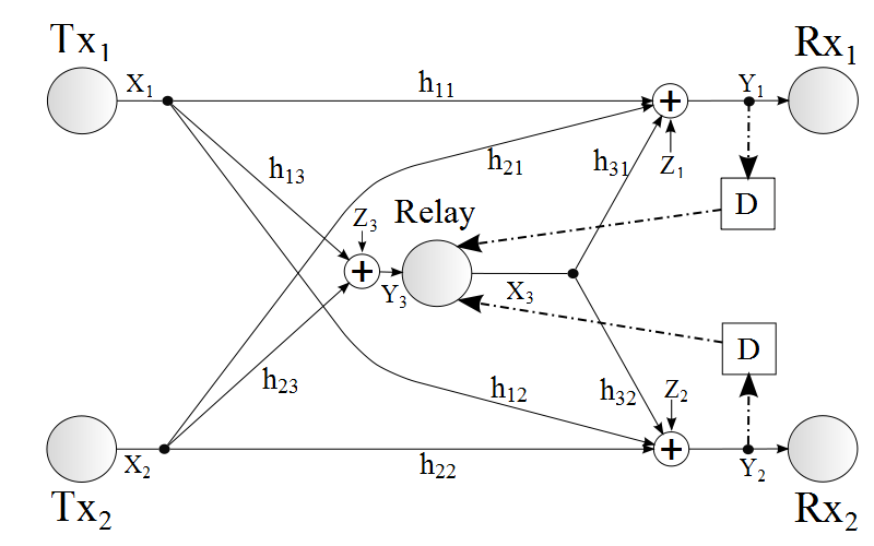
Figure 1: The interference channel with a relay and with feedback from both receivers to the relay. The ‘D’ block represents a single-symbol delay.

Throughout this paper channel state information (CSI) at the receivers is assumed. We represent the CSI at receiver $k$ with $\tilde{H}_{k}\triangleq\big{(}H_{1k},H_{2k},H_{3k}\big{)}$, $k\in\{1,2\}$. As each element in $\tilde{H}_{k}$ is a complex scalar random variable, then $\tilde{H}_{k}\in\mathfrak{C}^{3}$. For consistency of notations we use $\tilde{\mathfrak{H}}_{k}$ to denote the space of the random vector $\tilde{H}_{k}$, thus $\tilde{\mathfrak{H}}_{k}\equiv\mathfrak{C}^{3}$. In sections IV and V we assume noiseless feedback links from both receivers to the relay, s.t. the channel outputs $y_{1,1}^{i-1},y_{2,1}^{i-1}$, and the corresponding Rx-CSIs, $\tilde{h}_{1,1}^{i-1}$ and $\tilde{h}_{2,1}^{i-1}$, are available at the relay at time $i$ prior to transmission. This model is described in Fig. 1. Hence, the CSI at the relay is represented by $\underline{\tilde{H}}\triangleq\big{(}H_{13},H_{23},\tilde{H}_{1},\tilde{H}_{2}\big{)}\in\mathfrak{C}^{8}$. We denote the space of $\underline{\tilde{H}}$ with $\underline{\tilde{\mathfrak{H}}}\equiv\mathfrak{C}^{8}$.

Comment 1.

Note that as feedback contains both channel output and Rx-CSI, feedback from both receivers to the relay, leads to the relay having delayed Tx-CSI on its outgoing links. In this work we will show that as the channel is memoryless and the coefficients are i.i.d. with uniformly distributed phases, independent of their magnitudes, such feedback does not result in correlated channel inputs. Note that destinations-relay feedback which includes Rx-CSI leads to the conclusion that reliable decoding at the destinations guarantees reliable decoding at the relay. This, in turn, leads to the optimality of DF in SI and VSI. Without including Rx-CSI in the feedback signal, then, in order to achieve such an implication, it is necessary to impose restrictions on the channel coefficients. This decreases the set of channel coefficients for which we can achieve the capacity region of the ICRF by using DF at the relay. This will be elaborated upon in Comment 10.

Comment 2.

We note that an important problem is the case of global instantaneous CSI. In such a case, following the approach in [59] and [60], the fading channel is decomposed into parallel Gaussian ICRs. However, for such channels it is not possible to use the techniques of the current work to show that mutually independent channel inputs maximize the cut-set bound. This is because the channel coefficients and channel inputs at the same time instant can be correlated, and therefore the nodes can use the CSI to achieve correlation between their signals. The case of global instantaneous CSI will not be treated in the current manuscript.

We now define the code, probability of error, achievable rates, and capacity region:

Definition 1.

An $(R_{1},R_{2},n)$ code for the ICRF, depicted in Fig. 1, consists of two message sets $\mathcal{M}_{k}\triangleq\big{\{}1,2,...,2^{nR_{k}}\big{\}}$, $k\in\{1,2\}$, two encoders at the sources, $e_{1},e_{2}$, and two decoders at the destinations, $g_{1},g_{2}$; $e_{k}:\mathcal{M}_{k}\mapsto\mathfrak{C}^{n}$, $g_{k}:\tilde{\mathfrak{H}}_{k}^{n}\times\mathfrak{C}^{n}\mapsto\mathcal{M}_{k}$, $k\in\{1,2\}$. At the relay there is a causal encoder. Since in sections IV and V feedback from both receivers is available at the relay, then the encoded signal at the relay is a causal function of the channel outputs at the receivers, its own received symbols and the corresponding Rx-CSIs, i.e.,

$$x_{3,i}=t_{i}\big{(}y_{1,1}^{i-1},y_{2,1}^{i-1},y_{3,1}^{i-1},h_{13,1}^{i-1},h_{23,1}^{i-1},\tilde{h}_{1,1}^{i-1},\tilde{h}_{2,1}^{i-1}\big{)}\in\mathfrak{C},$$ (2)

$i=1,2,...,n$.

Definition 2.

The average probability of error is defined as $\makebox{P}_{e}^{(n)}\triangleq\Pr\big{(}g_{1}(\tilde{H}_{1}^{n},Y_{1}^{n})\neq M_{1}\mbox{ or }g_{2}(\tilde{H}_{2}^{n},Y_{2}^{n})\neq M_{2}\big{)}$, where $M_{1}$ and $M_{2}$ are selected independently and uniformly over their message sets.

Definition 3.

A rate pair $(R_{1},R_{2})$ is called achievable if for any $\epsilon>0$ and $\delta>0$ there exists some block length $n_{0}(\epsilon,\delta)$ s.t. for every integer $n>n_{0}(\epsilon,\delta)$ there exists an $(R_{1}-\delta,R_{2}-\delta,n)$ code with $\makebox{P}_{e}^{(n)}<\epsilon$.

Definition 4.

The capacity region is defined as the convex hull of all achievable rate pairs.

In sections VI and VII, the definitions of Rx-CSI and the code will be specialized according to the feedback configurations of these sections.

In this paper we also present explicit capacity expressions for phase fading and Rayleigh fading models, which are two fading models that satisfy the general fading model defined above. These models are defined as follows:

• Phase fading channels: The channel coefficients are given by $H_{lk,i}=a_{lk}e^{j\Theta_{lk,i}}$, $a_{lk}\in\mathfrak{R}_{+}$ are non-negative constants corresponding to the attenuation of the signal power from node $l$ to node $k$, and $\Theta_{lk,i}$ are uniformly distributed over $[0,2\pi)$, independent in time and independent of each other and of the additive noises $Z_{k}$, $k\in\{1,2,3\}$.

• Rayleigh fading channels: The channel coefficients are given by $H_{lk,i}=a_{lk}U_{lk,i}$ , $a_{lk}\in\mathfrak{R}_{+}$ are non-negative constants corresponding to the attenuation of the signal power from node $l$ to node $k$, and $U_{lk,i}$ are circularly symmetric, complex Normal RVs, $U_{lk,i}\sim\mathcal{CN}(0,1)$, independent in time and independent of each other and of the additive noises $Z_{k}$, $k\in\{1,2,3\}$.

III Preliminaries

In this section we present some of the frequently used lemmas.

III-A Maximum Entropy for Complex Random Vectors

Lemma 1.

Consider a complex random vector, $\mathbf{X}\triangleq(\mathbf{X}_{1},\mathbf{X}_{2})$. Let $\mathbf{X}^{\prime}\triangleq(\mathbf{X}^{\prime}_{1},\mathbf{X}^{\prime}_{2})=\mathbf{X}-\mathds{E}\{\mathbf{X}\}$. Then $h(\mathbf{X}^{\prime}_{1}|\mathbf{X}^{\prime}_{2})=h(\mathbf{X}_{1}|\mathbf{X}_{2})$.

Proof.

The proof follows directly from the definition of the differential entropy. ∎

Lemma 2.

Let $X_{1},X_{2},...,X_{k}$ be an arbitrary set of $k$ zero-mean complex random variables with covariance matrix $\mathds{K}$. Let $\mathcal{S}$ be any subset of $n$ elements from $\{1,2,...,k\}$ and $\mathcal{S}^{C}$ be its complement. Then:

$$h(\mathbf{X}_{\mathcal{S}}|\mathbf{X}_{\mathcal{S}^{C}})\leq\log\Big{(}(\pi e)^{n}\det\big{(}\textnormal{cov}(\mathbf{X}_{\mathcal{S}}|\mathbf{X}_{\mathcal{S}^{C}})\big{)}\Big{)},$$

with equality if and only if $X_{1},X_{2},...,X_{k}\sim\mathcal{CN}(0,\mathds{K})$.

Proof.

The proof follows along the lines of the proof of [49, Lemma 1] and an application of [34, Theorem 1] and [34, Theorem 2]. ∎

III-B The Positive Semidefinite Ordering

Lemma ([46, Lemma 3.1]).

Let $\mathbf{X_{1}}$ and $\mathbf{X_{2}}$ be random vectors with zero mean and covariance matrices $\mathds{C}_{mk}\triangleq\mathds{E}\{\mathbf{X}_{m}\mathbf{X}^{H}_{k}\},m,k\in\{1,2\}$. Define: $\mathds{A}\triangleq\mathds{C}^{-\frac{1}{2}}_{11}\cdot\mathds{C}_{12}\cdot\mathds{C}^{-\frac{1}{2}}_{22}$. Then there exists $\rho\in[0,1]$ s.t.

$$\mathds{I}-\mathds{A}\mathds{A}^{H}\preceq(1-\rho^{2})\mathds{I}.$$

III-C Joint Typicality

Lemma ([6, Lemma 2]).

Let $(\mathbf{S}_{1},\mathbf{S}_{2},\mathbf{S}_{3})\sim\prod_{i=1}^{n}p(s_{1,i},s_{2,i},s_{3,i})$ and ${(\mathbf{S}^{\prime}_{1},\mathbf{S}^{\prime}_{2},\mathbf{S}_{3})\sim\prod_{i=1}^{n}p(s_{3,i})\times}$ $p(s_{1,i}|s_{3,i})p(s_{2,i}|s_{3,i})$. Then for $n$ s.t. $\Pr\big{\{}A^{n}_{\epsilon}(\mathbf{S}_{1},\mathbf{S}_{2},\mathbf{S}_{3})\big{\}}\geq 1-\epsilon$, it holds that:

$$\Pr\big{\{}(\mathbf{S}^{\prime}_{1},\mathbf{S}^{\prime}_{2},\mathbf{S}_{3})\in A^{(n)}_{\epsilon}(\mathbf{S}_{1},\mathbf{S}_{2},\mathbf{S}_{3})\big{\}}$$

$$\quad\qquad\qquad\qquad\qquad\qquad\qquad\leq 2^{-n\big{(}I(S_{1};S_{2}|S_{3})-7\epsilon\big{)}}.$$

III-D The Capacity of Phase Fading and of Rayleigh Fading MIMO Relay Channels

We now state a slight variation of [7, Theorem. 8] which will be used in this paper:

Theorem ([7, Theorem. 8]).

For phase fading and for Rayleigh fading relay channels with multiple antennas, and with Rx-CSI available, the channel inputs $\tilde{{X}}_{1}$ and $\tilde{{X}}_{3}$ that maximize both the cut-set bound,

$$\max_{p(\tilde{{x}}_{1},\tilde{{x}}_{3})}\min\big{\{}I(\tilde{{X}}_{1};\tilde{Y}_{1},\tilde{Y}_{3}|\tilde{{X}}_{3},\tilde{H}_{11},\tilde{H}_{31},\tilde{H}_{13}),$$

$$\qquad\qquad\qquad\qquad\qquad I(\tilde{{X}}_{1},\tilde{{X}}_{3};\tilde{Y}_{1}|\tilde{H}_{11},\tilde{H}_{31})\big{\}},$$

and the DF rate, $\max_{p(\tilde{{x}}_{1},\tilde{{x}}_{3})}\min\big{\{}I(\tilde{{X}}_{1};\tilde{Y}_{3}|\tilde{{X}}_{3},\tilde{H}_{13}),$ $I(\tilde{{X}}_{1},\tilde{{X}}_{3};\tilde{Y}_{1}|\tilde{H}_{11},\tilde{H}_{31})\big{\}}$, are independent complex Normal variables. The best covariance matrix for transmitter $\mbox{Tx}_{t}$ is $\mathds{Q}_{\tilde{{X}}_{t}}=\sqrt{\frac{P_{t}}{n_{t}}}\mathds{I}_{n_{t}}$, $t=1,2$, where $\mathds{I}_{n_{t}}$ is the $n_{t}\times n_{t}$ identity matrix. DF achieves capacity if its rate is $I(\tilde{{X}}_{1},\tilde{{X}}_{3};\tilde{Y}_{1})$. The capacity is then given by

$$C_{\mbox{\scriptsize fading relay}} = \int_{\tilde{h}_{\mathcal{T}},1}f(\tilde{h}_{\mathcal{T},1})\log_{2}\bigg{|}\mathds{I}_{l_{1}}+a_{11}^{2}\frac{P_{1}}{n_{1}}\tilde{h}_{11}\tilde{h}_{11}^{H}$$

$$\qquad\qquad\qquad\qquad+a_{31}^{2}\frac{P_{3}}{n_{3}}\tilde{h}_{31}\tilde{h}_{31}^{H}\bigg{|}d\tilde{h}_{\mathcal{T},1},$$

where $\tilde{h}_{\mathcal{T},1}\triangleq\big{\{}\tilde{h}_{11},\tilde{h}_{31}\big{\}}$.

IV ICRFs in the Very Strong Interference Regime

In this section, we consider the ICRF with two noiseless feedback links from the receivers to the relay (see Fig. 1) and we characterize the capacity region of ICRFs in the VSI regime. This result is stated in the following theorem:

Theorem 1.

Consider the fading ICRF with Rx-CSI. Assume that the channel coefficients are independent in time and independent of each other s.t. their phases are i.i.d. and distributed uniformly over $[0,2\pi)$. Let the additive noises be i.i.d. circularly symmetric complex Normal processes, $\mathcal{CN}(0,1)$, and let the sources have power constraints $\mathds{E}\big{\{}|X_{k}|^{2}\big{\}}\leq P_{k}$, $k\in\{1,2,3\}$. Assume noiseless feedback links from both receivers to the relay (see Fig. 1). If

$$I(X_{1},X_{3};Y_{1}|X_{2},\tilde{H}_{1}) \leq I(X_{1};Y_{2}|\tilde{H}_{2})$$ (3a)

$$I(X_{2},X_{3};Y_{2}|X_{1},\tilde{H}_{2}) \leq I(X_{2};Y_{1}|\tilde{H}_{1}),$$ (3b)

where the mutual information expressions are evaluated with $X_{k}\sim\mathcal{CN}(0,P_{k}),k\in\{1,2,3\}$, mutually independent, then the capacity region is given by all the nonnegative rate pairs s.t.

$$R_{1} \leq I(X_{1},X_{3};Y_{1}|X_{2},\tilde{H}_{1})$$ (4a)

$$R_{2} \leq I(X_{2},X_{3};Y_{2}|X_{1},\tilde{H}_{2}),$$ (4b)

and it is achieved with $X_{k}\sim\mathcal{CN}(0,P_{k}),k\in\{1,2,3\}$, mutually independent and with DF strategy at the relay.

IV-A Proof of Theorem 1

The proof consists of the following steps:

• We obtain an outer bound on the capacity region using the cut-set bound.

• We show that the input distribution that maximizes the outer bound is zero-mean, circularly symmetric complex Normal with channel inputs independent of each other and with maximum allowed power.

• We derive an achievable rate region based on DF at the relay and by using mutually independent codebooks generated according to the zero-mean, circularly symmetric complex Normal input distribution:

  • We derive an achievable rate region for decoding at the relay using steps similar to [7, Sec. 4.D].

  • We obtain an achievable rate region for decoding at the destination by decoding the interference first, while treating the relay signal and the desired signal as additive i.i.d. noises, followed by using a backward decoding scheme for decoding the desired message.

• We derive the VSI conditions which guarantee that decoding the interference first at each receiver, does not constrain the rate of the other pair.

• We conclude that when the VSI conditions hold the achievable region coincides with the cut-set bound.

These steps are elaborated in sections IV-A1, IV-A2 and IV-A3.

IV-A1 An Outer Bound

The cut-set theorem [39, Theorem 15.10.1] applied to the ICRF results in the following upper bounds:

$$\mathcal{S} \triangleq \{\mbox{Tx}_{1}\},\mathcal{S}^{C}\triangleq\{\mbox{Tx}_{2},\mbox{Relay},\mbox{Rx}_{1},\mbox{Rx}_{2}\}:$$ (5a)

$$\quad R_{1}\leq I(X_{1};Y_{1},Y_{2},Y_{3}|X_{2},X_{3},\underline{\tilde{H}})$$

$$\mathcal{S} \triangleq \{\mbox{Tx}_{1},\mbox{Relay},\mbox{Rx}_{2}\},\mathcal{S}^{C}\triangleq\{\mbox{Tx}_{2},\mbox{Rx}_{1}\}:$$ (5b)

$$\quad R_{1}\leq I(X_{1},X_{3};Y_{1}|X_{2},\tilde{H}_{1})$$

$$\mathcal{S} \triangleq \{\mbox{Tx}_{2}\},\mathcal{S}^{C}\triangleq\{\mbox{Tx}_{1},\mbox{Relay},\mbox{Rx}_{1},\mbox{Rx}_{2}\}:$$ (5c)

$$\quad R_{2}\leq I(X_{2};Y_{1},Y_{2},Y_{3}|X_{1},X_{3},\underline{\tilde{H}})$$

$$\mathcal{S} \triangleq \{\mbox{Tx}_{2},\mbox{Relay},\mbox{Rx}_{1}\},\mathcal{S}^{C}\triangleq\{\mbox{Tx}_{1},\mbox{Rx}_{2}\}:$$ (5d)

$$\quad R_{2}\leq I(X_{2},X_{3};Y_{2}|X_{1},\tilde{H}_{2})$$

$$\mathcal{S} \triangleq \{\mbox{Tx}_{1},\mbox{Tx}_{2}\},\mathcal{S}^{C}\triangleq\{\mbox{Rx}_{1},\mbox{Rx}_{2},\mbox{Relay}\}:$$ (5e)

$$\quad R_{1}+R_{2}\leq I(X_{1},X_{2};Y_{1},Y_{2},Y_{3}|X_{3},\underline{\tilde{H}}).$$

Next, we find the channel input distribution that maximizes the cut-set bound. We follow the same approach as in [7, Proposition 2] and [7, Theorem 8]. Let $\mathbf{X}$ denote the channel inputs with the maximizing distribution. Note that Lemma 1 states that the zero-mean complex random vector $\mathbf{X}^{\prime}\triangleq\mathbf{X}-\mathds{E}\{\mathbf{X}\}$ has the same entropy as $\mathbf{X}$. Hence, the most efficient strategy would be to transmit $\mathbf{X}^{\prime}$ rather than $\mathbf{X}$, since subtracting the average reduces the power consumption. Using the steps detailed in Appendix A, we conclude that each mutual information expression in (5) is maximized by (zero-mean) circularly symmetric complex Normal channel inputs, independent of each other, and with the sources transmitting at their maximum available power even though the scenario consists of a combination of relaying and feedback.

Comment 3.

Note that this conclusion is not immediate from [7, Theorem 8], since in the ICRF there are two destinations, while the cut-set bound in [7, Theorem 8] considers only one destination and $T$ transmitting relays. Hence, the conditional entropies in the present case contain more complicated combinations of the correlation coefficients between the channel inputs and thus each expression needs to be examined individually.

Comment 4.

Note that although the cut-set bound of the ICRF scenario requires maximization over all input distributions of the type $f(x_{1})f(x_{2})f(x_{3}|x_{1},x_{2})$, in Appendix A it is shown that $f(x_{3}|x_{1},x_{2})=f(x_{3})$ is the maximizing distribution at the relay, and that the input distribution is jointly Gaussian (as follows from [7, Proposition 2]). The intuition behind the mathematical result is that as receivers have Rx-CSI, then the mutual information expressions involve averaging over all channel coefficients. However, as the phases are all uniformly distributed over $[0,2\pi)$, it follows that for any cross-correlation structure between the channel inputs, the same rate bounds can be obtained by the negative cross-correlation. Thus the maximum rate is achieved when the cross-correlations are equal to their negatives, and are therefore zero. As the maximizing distribution is uncorrelated Gaussians, they are also independent. This also reflects the fact that due to the i.i.d. uniform phase of the fading process, it is not possible to correlate the channel codewords of the different transmitting nodes, leading, due to Gaussianity, to independence.

IV-A2 An Achievable Rate Region

Now we obtain an achievable rate region using the input distribution that maximizes the cut-set bound in (5). The achievability is based on DF strategy at the relay. Fix the blocklength $n$ and the input distribution $f_{X_{1},X_{2},X_{3}}(x_{1},x_{2},x_{3})=f_{X_{1}}(x_{1})\cdot f_{X_{2}}(x_{2})\cdot f_{X_{3}}(x_{3})$ where $f_{X_{k}}(x_{k})\sim\mathcal{CN}(0,P_{k}),k=1,2,3$. Consider the following coding scheme, in which $B-1$ messages are transmitted using $nB$ channel symbols:

Code Construction

For each message $m_{k}\in\mathcal{M}_{k},k\in\{1,2\}$ select a codeword $\mathbf{x}_{k}(m_{k})$ according to the p.d.f. $f_{\mathbf{X}_{k}}\big{(}\mathbf{x}_{k}(m_{k})\big{)}=\prod_{i=1}^{n}f_{X_{k}}\big{(}x_{k,i}(m_{k})\big{)}$. For each $(m_{1},m_{2})\in\mathcal{M}_{1}\times\mathcal{M}_{2}$ select a codeword $\mathbf{x}_{3}(m_{1},m_{2})$ according to the p.d.f. $f_{\mathbf{X}_{3}}\big{(}\mathbf{x}_{3}(m_{1},m_{2})\big{)}=\prod_{i=1}^{n}f_{X_{3}}\big{(}x_{3,i}(m_{1},m_{2})\big{)}$.

Encoding at Block $b$

At block $b$, Tx_k transmits $m_{k,b}$ using $\mathbf{x}_{k}(m_{k,b}),k\in\{1,2\}$. Let $(\hat{m}_{1,b-1},\hat{m}_{2,b-1})$ denote the decoded ($m_{1,b-1},m_{2,b-1}$) at block $b-1$ at the relay. At block $b$ the relay transmits $\mathbf{x}_{3}(\hat{m}_{1,b-1},\hat{m}_{2,b-1})$. At block $b=1$ the relay transmits $\mathbf{x}_{3}(1,1)$, and at block $b=B$, Tx₁ and Tx₂ transmit $\mathbf{x}_{1}(1)$ and $\mathbf{x}_{2}(1)$, respectively.

Decoding at the Relay at Block $b$

Decoding at the relay is very similar to the MARC case studied in [7, Sec. 4.D], the difference being that here feedback is available at the relay. In the present case, the relay uses its knowledge of $\mathbf{Y}_{1}(b),\mathbf{Y}_{2}(b),\mathbf{Y}_{3}(b)$ and $\mathbf{\underline{\tilde{H}}}(b)$ to decode $(m_{1,b},m_{2,b})$ by using a joint-typicality decoder. The decoder looks for a unique pair, $(m_{1},m_{2})\in\mathcal{M}_{1}\times\mathcal{M}_{2}$ that satisfies:

$$\!\!\!\!\!\!\!\!\!\!\Big{(}\mathbf{x}_{1}(m_{1}),\mathbf{x}_{2}(m_{2}),\mathbf{x}_{3}(m_{1,b-1},m_{2,b-1}),\mathbf{y}_{1}(b),\mathbf{y}_{2}(b),$$

$$\mathbf{y}_{3}(b),\mathbf{\underline{\tilde{h}}}(b)\Big{)}\in A_{\epsilon}^{(n)}(X_{1},X_{2},X_{3},Y_{1},Y_{2},Y_{3},\underline{\tilde{H}}).$$ (6)

Following the analysis in [7, Sec. 4.D], it is concluded that the achievable rate region for decoding at the relay is given by:

$$\!\!\!\!\!\!\!\!\!\!\!\!\!\!\!\!\!\!\mathcal{R}_{\mbox{\scriptsize{Relay Decoding}}}=$$

$$\!\!\!\!\!\!\!\!\!\!\!\!\bigg{\{}(R_{1},R_{2})\in\mathfrak{R}^{2}_{+}:$$

$$\;R_{1}\leq I(X_{1};Y_{1},Y_{2},Y_{3}|X_{2},X_{3},\underline{\tilde{H}})$$

$$\;R_{2}\leq I(X_{2};Y_{1},Y_{2},Y_{3}|X_{1},X_{3},\underline{\tilde{H}})$$

$$\;R_{1}+R_{2}\leq I(X_{1},X_{2};Y_{1},Y_{2},Y_{3}|X_{3},\underline{\tilde{H}})\bigg{\}}.$$ (7a)

Decoding at the Destinations at Block $b$

The receivers use a backward block decoding method as in [7, Appendix A]. Assume that each receiver has correctly decoded $(m_{1,b+1},m_{2,b+1})$. Recall that the codebooks are generated independently, thus, in order to decode $m_{k,b},k\in\{1,2\}$ each receiver first decodes the interference, i.e., Rx₁ decodes $m_{2,b}$ and Rx₂ decodes $m_{1,b}$ by treating the signal from the relay and its own desired signal as i.i.d. additive noise, independent of the interfering signal, which holds by construction of the codebooks and by the i.i.d. channel assumption. Note that for this decoding step the channel is treated as a PtP channel, the capacity of which is derived in [39, Ch. 7.1]. Thus, due to Rx-CSI, Rx₁ can decode the interference if

$$R_{2}\leq I(X_{2};Y_{1}|\tilde{H}_{1}),$$ (8a)

and Rx₂ can decode the interference if

$$R_{1}\leq I(X_{1};Y_{2}|\tilde{H}_{2}).$$ (8b)

After decoding the interference, each receiver uses its CSI to decode its desired message. We consider the decoding process at Rx₁; the decoding process at Rx₂ follows the same steps.

• Rx₁ generates the sets:

  $$\!\!\!\!\!\!\!\!\!\!\!\!\mathcal{E}_{0,b} \triangleq \Big{\{}m_{1}\in\mathcal{M}_{1}:\big{(}\mathbf{x}_{1}(m_{1,b+1}),\mathbf{x}_{2}(m_{2,b+1}),$$

  $$\;\mathbf{x}_{3}(m_{1},\hat{m}_{2,b}),\mathbf{y}_{1}(b+1),\mathbf{\tilde{h}}_{1}(b+1)\big{)}\in A_{\epsilon}^{(n)}\Big{\}}.$$

  $$\!\!\!\!\!\!\!\!\!\!\!\!\mathcal{E}_{1,b} \triangleq \Big{\{}m_{1}\in\mathcal{M}_{1}:\big{(}\mathbf{x}_{1}(m_{1}),\mathbf{x}_{2}(\hat{m}_{2,b}),$$

  $$\;\qquad\qquad\qquad\mathbf{y}_{1}(b),\mathbf{\tilde{h}}_{1}(b)\big{)}\in A_{\epsilon}^{(n)}\Big{\}}.$$

• Rx₁ then decodes $m_{1,b}$ by finding a unique $m_{1}\in\mathcal{E}_{0,b}\cap\mathcal{E}_{1,b}$.

Note that since the codewords are independent of each other, $\mathcal{E}_{0,b}$ is independent of $\mathcal{E}_{1,b}$. Thus, assuming $\hat{m}_{2,b}=m_{2,b}$, and using standard joint-typicality arguments [39, Theorem. 7.6.1], it follows that the probability of decoding error can be made arbitrarily small by taking $n$ large enough as long as

$$R_{1} \leq I(X_{1};Y_{1}|X_{2},\tilde{H}_{1})+I(X_{3};Y_{1}|X_{1},X_{2},\tilde{H}_{1})$$ (9a)

$$= I(X_{1},X_{3};Y_{1}|X_{2},\tilde{H}_{1}),$$

and for decoding at Rx₂ we obtain

$$R_{2}\leq I(X_{2},X_{3};Y_{2}|X_{1},\tilde{H}_{2}).$$ (9b)

Combining with (8) we conclude that subject to reliable decoding at the relay, the achievable rate region for decoding at the destinations is characterized by:

$$\!\!\!\!\!\!\!\!\!\!\!\!\!\!\!\!\!\!\mathcal{R}^{\prime}_{\mbox{\scriptsize{Destination Decoding}}}$$

$$\!\!\!\!\!\!\!\!\!\!\!\!=\bigg{\{}(R_{1},R_{2})\in\mathfrak{R}^{2}_{+}:$$

$$\;\;R_{1}\leq\min\big{\{}I(X_{1},X_{3};Y_{1}|X_{2},\tilde{H}_{1}),$$

$$\;\;\qquad\qquad\qquad\qquad I(X_{1};Y_{2}|\tilde{H}_{2})\big{\}}$$ (10a)

$$\;\;R_{2}\leq\min\big{\{}I(X_{2},X_{3};Y_{2}|X_{1},\tilde{H}_{2}),$$

$$\;\;\qquad\qquad\qquad\qquad I(X_{2};Y_{1}|\tilde{H}_{1})\big{\}}\bigg{\}}.$$ (10b)

Hence, an achievable rate region is obtained by

$$\mathcal{R}_{\mbox{\scriptsize{Achievable}}}=\mathcal{R}_{\mbox{\scriptsize{Relay Decoding}}}\cap\mathcal{R}^{\prime}_{\mbox{\scriptsize{Destination Decoding}}}.$$ (11)

IV-A3 Capacity Region for the Very Strong Interference Regime

Now we obtain the conditions on the channel coefficients which guarantee that the interference is strong enough s.t. the receivers can decode the interference without reducing the rate region. Combining (7) and (10) with (8), we obtain the VSI conditions for the ICRF:

$$\!\!\!\!\!\!\!\!\!\!\!\!\min\big{\{}I(X_{1};Y_{1},Y_{2},Y_{3}|X_{2},X_{3},\underline{\tilde{H}}),$$

$$\quad I(X_{1},X_{3};Y_{1}|X_{2},\tilde{H}_{1})\big{\}}\leq I(X_{1};Y_{2}|\tilde{H}_{2})$$ (12a)

$$\!\!\!\!\!\!\!\!\!\!\!\!\min\big{\{}I(X_{2};Y_{1},Y_{2},Y_{3}|X_{1},X_{3},\underline{\tilde{H}}),$$

$$\quad I(X_{2},X_{3};Y_{2}|X_{1},\tilde{H}_{2})\big{\}}\leq I(X_{2};Y_{1}|\tilde{H}_{1}).$$ (12b)

Thus, when (12) holds the achievable region is given by (9) and (7). Note that since the codebooks are independent of each other and of the channel coefficients,

$$I(X_{1};Y_{2}|\tilde{H}_{2}) = h(X_{1}|\tilde{H}_{2})-h(X_{1}|Y_{2},\tilde{H}_{2})$$ (13a)

$$= h(X_{1}|X_{2},X_{3},\tilde{H}_{2})-h(X_{1}|Y_{2},\tilde{H}_{2})$$

$$\leq h(X_{1}|X_{2},X_{3},\underline{\tilde{H}})$$

$$-h(X_{1}|Y_{1},Y_{2},Y_{3},X_{2},X_{3},\underline{\tilde{H}})$$

$$= I(X_{1};Y_{1},Y_{2},Y_{3}|X_{2},X_{3},\underline{\tilde{H}}),$$

we also obtain

$$I(X_{2};Y_{1}|\tilde{H}_{1})\leq I(X_{2};Y_{1},Y_{2},Y_{3}|X_{1},X_{3},\underline{\tilde{H}}).$$ (13b)

Hence, the conditions in (12) reduce to

$$I(X_{1},X_{3};Y_{1}|X_{2},\tilde{H}_{1}) \leq I(X_{1};Y_{2}|\tilde{H}_{2})$$ (14a)

$$I(X_{2},X_{3};Y_{2}|X_{1},\tilde{H}_{2}) \leq I(X_{2};Y_{1}|\tilde{H}_{1}),$$ (14b)

which give (3). Next, note that (13) and (14) imply that the achievable region is characterized by (9) and (7a). However, when (13) and (14) hold, then

$$\!\!\!\!\!\!\!I(X_{1},X_{2};Y_{1},Y_{2},Y_{3}|X_{3},\underline{\tilde{H}})$$

$$=I(X_{2};Y_{1},Y_{2},Y_{3}|X_{3},\underline{\tilde{H}})$$

$$\qquad+I(X_{1};Y_{1},Y_{2},Y_{3}|X_{2},X_{3},\underline{\tilde{H}})$$

$$\geq I(X_{2};Y_{1}|\tilde{H}_{1})+I(X_{1};Y_{2}|\tilde{H}_{2})$$

$$\geq I(X_{2},X_{3};Y_{2}|X_{1},\tilde{H}_{2})+I(X_{1},X_{3};Y_{1}|X_{2},\tilde{H}_{1}).$$

Therefore, we see that in the VSI regime, the sum-rate condition, (7a), is always satisfied. We conclude that when (3) holds, (4) defines the achievable region. Finally, note that the rate region characterized by (4) coincides with the cut-set bound in section IV-A1 (since (4) is only a subset of the constraints but it is achievable), hence it is the capacity region of the ICRF in the VSI regime.

$\blacksquare$

IV-B Ergodic Phase Fading

The capacity region of ICRFs under ergodic phase fading in the VSI regime is characterized explicitly in the following corollary:

Corollary 1.

Consider the phase fading ICRF with Rx-CSI and noiseless feedback links from both receivers to the relay, s.t. $y_{1,1}^{i-1},y_{2,1}^{i-1},\tilde{h}_{1,1}^{i-1}$ and $\tilde{h}_{2,1}^{i-1}$ are available at the relay at time $i$. If the channel coefficients satisfy

$$a_{11}^{2}P_{1}+a_{31}^{2}P_{3} \leq \frac{a_{12}^{2}P_{1}}{1+a_{22}^{2}P_{2}+a_{32}^{2}P_{3}}$$ (15a)

$$a_{22}^{2}P_{2}+a_{32}^{2}P_{3} \leq \frac{a_{21}^{2}P_{2}}{1+a_{11}^{2}P_{1}+a_{31}^{2}P_{3}},$$ (15b)

then the capacity region is characterized by all the nonnegative rate pairs s.t.

$$R_{1} \leq \log_{2}\big{(}1+a_{11}^{2}P_{1}+a_{31}^{2}P_{3}\big{)}$$ (16a)

$$R_{2} \leq \log_{2}\big{(}1+a_{22}^{2}P_{2}+a_{32}^{2}P_{3}\big{)},$$ (16b)

and it is achieved with $X_{k}\sim\mathcal{CN}(0,P_{k}),k\in\{1,2,3\}$, mutually independent and with DF strategy at the relay.

Proof.

The proof follows from the expressions of Theorem 1. In order to obtain the conditions on the channel coefficients in (15), we evaluate $I(X_{1},X_{3};Y_{1}|X_{2},\tilde{H}_{1})$ and $I(X_{2},X_{3};Y_{2}|X_{1},\tilde{H}_{2})$ using the right-hand side (r.h.s.) of equation (A-A) in Appendix A. Recall that the channel inputs that maximize these expressions are mutually independent, zero mean, circularly symmetric complex Normal and with maximum power. Thus, we obtain

$$I(X_{1},X_{3};Y_{1}|X_{2},\tilde{H}_{1}) = \log_{2}(1+a_{11}^{2}P_{1}+a_{31}^{2}P_{3})$$

$$I(X_{2},X_{3};Y_{2}|X_{1},\tilde{H}_{2}) = \log_{2}(1+a_{22}^{2}P_{2}+a_{32}^{2}P_{3}).$$

Note that for evaluating the r.h.s. of (3), $\{H_{31,i}X_{3,i}\}_{i=1}^{n}$ and $\{H_{11,i}X_{1,i}\}_{i=1}^{n}$ are treated as additive Gaussian noises at Rx₁ and $\{H_{32,i}X_{3,i}\}_{i=1}^{n}$ and $\{H_{22,i}X_{2,i}\}_{i=1}^{n}$ are treated as additive Gaussian noises at Rx₂. Hence, we obtain

$$I(X_{2};Y_{1}|\tilde{H}_{1}) = \log_{2}\Big{(}1+\frac{a_{21}^{2}P_{2}}{1+a_{11}^{2}P_{1}+a_{31}^{2}P_{3}}\Big{)}$$

$$I(X_{1};Y_{2}|\tilde{H}_{2}) = \log_{2}\Big{(}1+\frac{a_{12}^{2}P_{1}}{1+a_{22}^{2}P_{2}+a_{32}^{2}P_{3}}\Big{)}.$$

Thus (3) results in conditions (15) and (4) results in (16). ∎

IV-C Ergodic Rayleigh Fading

In this section the capacity region of ICRFs under ergodic Rayleigh fading in the VSI regime is characterized. Define $\tilde{U}_{k}\triangleq(U_{kk},U_{3k}),k\in\{1,2\}$ and define $E_{1}(x)$ as in [36, Eqn. 5.1.1]:

$$E_{1}(x)\triangleq\int^{\infty}_{x}\frac{e^{-t}}{t}dt.$$

Corollary 2.

Consider the Rayleigh fading ICRF with Rx-CSI and noiseless feedback links from both receivers to the relay, s.t. $y_{1,1}^{i-1},y_{2,1}^{i-1},\tilde{h}_{1,1}^{i-1}$ and $\tilde{h}_{2,1}^{i-1}$ are available at the relay at time $i$. If the channel coefficients satisfy

$$\!\!\!\!\!\!\!\!\frac{\frac{a_{12}^{2}P_{1}}{1+a_{22}^{2}P_{2}+a_{32}^{2}P_{3}}}{e^{\frac{1+a_{22}^{2}P_{2}+a_{32}^{2}P_{3}}{a_{12}^{2}P_{1}}}E_{1}\left(\frac{1+a_{22}^{2}P_{2}+a_{32}^{2}P_{3}}{a_{12}^{2}P_{1}}\right)}$$

$$\qquad\qquad\qquad\geq(1+a_{11}^{2}P_{1}+a_{31}^{2}P_{3})$$ (17a)

$$\!\!\!\!\!\!\!\!\frac{\frac{a_{21}^{2}P_{2}}{1+a_{11}^{2}P_{1}+a_{31}^{2}P_{3}}}{e^{\frac{1+a_{11}^{2}P_{1}+a_{31}^{2}P_{3}}{a_{21}^{2}P_{2}}}E_{1}\left(\frac{1+a_{11}^{2}P_{1}+a_{31}^{2}P_{3}}{a_{21}^{2}P_{2}}\right)}$$

$$\qquad\qquad\qquad\geq(1+a_{22}^{2}P_{2}+a_{32}^{2}P_{3}),$$ (17b)

then the capacity region is characterized by all the nonnegative rate pairs s.t.

$$\!\!\!\!\!\!\!\!\!\!\!\!R_{1} \!\leq \!\mathds{E}_{\tilde{U}_{1}}\!\big{\{}\log_{2}(1+a_{11}^{2}|U_{11}|^{2}P_{1}+a_{31}^{2}|U_{31}|^{2}P_{3})\big{\}}$$ (18a)

$$\!\!\!\!\!\!\!\!\!\!\!\!R_{2} \!\leq \!\mathds{E}_{\tilde{U}_{2}}\!\big{\{}\log_{2}(1+a_{22}^{2}|U_{22}|^{2}P_{2}+a_{32}^{2}|U_{32}|^{2}P_{3})\big{\}},$$ (18b)

and it is achieved with $X_{k}\sim\mathcal{CN}(0,P_{k}),k\in\{1,2,3\}$, mutually independent and with DF strategy at the relay.

Proof.

The proof follows the same approach as in Corollary 1. The detailed calculation of (17) can be found in [18]. Recall that for Rayleigh fading, the channel coefficients are complex Normal RVs. Thus, for decoding the interference at the receivers, $H_{31}X_{3},H_{11}X_{1},H_{32}X_{3}$ and $H_{22}X_{2}$ cannot be treated as additive Gaussian noises. Hence, the mutual information expressions on the r.h.s. of (3) need to be bounded using the $E_{1}$ function. ∎

IV-D Comments

Comment 5.

We now compare the capacity region of the ICRF in VSI to the ICR without feedback in VSI. First, consider the phase fading model, and define the set of coefficients $\mathcal{D}_{PF}$ as follows:

$$\!\!\!\!\!\!\!\!\!\!\!\!\!\!\!\!\!\!\!\!\mathcal{D}_{PF}\triangleq\Big{\{}(a_{31},a_{13},a_{32},a_{23})\in\mathfrak{R}_{+}^{4}:$$

$$\qquad\qquad a_{11}^{2}P_{1}+a_{31}^{2}P_{3}\leq a_{13}^{2}P_{1}$$ (19a)

$$\qquad\qquad a_{22}^{2}P_{2}+a_{32}^{2}P_{3}\leq a_{23}^{2}P_{2}$$ (19b)

$$\!\!\!\!\!\!\!(1\!+a_{11}^{2}P_{1}\!+a_{31}^{2}P_{3})(1\!+a_{22}^{2}P_{2}\!+\!a_{32}^{2}P_{3})$$

$$\qquad\qquad\qquad\leq 1\!+\!a_{13}^{2}P_{1}\!+\!a_{23}^{2}P_{2}\Big{\}}.$$ (19c)

In [17, Theorem 1] it is shown that when the channel coefficients satisfy (15) and $(a_{31},a_{13},a_{32},a_{23})\in\mathcal{D}_{PF}$, then capacity of the ICR is given by (16). Note that $(a_{31},a_{13},a_{32},a_{23})\in\mathcal{D}_{PF}$ implies that the links from the transmitters to the relay are good in the sense that if a rate pair can be reliably decoded at the destinations, then, it can also be reliably decoded at the relay. Observe that feedback does not affect the rate constraints (16), thus, when capacity is achieved without any feedback, then additional feedback links from each receiver to the relay do not enlarge the capacity region. Hence, the main benefit of feedback to the relay is that it allows to achieve capacity in VSI for any quality of links from the transmitters to the relay. Therefore, the set of channel coefficients for which capacity is achieved is defined only by (15) without the additional restrictions of $\mathcal{D}_{PF}$.

We also note that for the ICRF, when (15) holds, the cut-set bound is given by (16). Consider next the ICR in which (15) holds yet $(a_{31},a_{13},a_{32},a_{23})\notin\mathcal{D}_{PF}$. Taking $a_{13},a_{23}\rightarrow 0$, we eventually obtain that the cut-set bound (see [18, Eqn. (C.1)]) is a subset of (16). For such scenarios, feedback enlarges the capacity region compared to the no-feedback case. Similar conclusions hold also for Rayleigh fading.

Comment 6.

Fig. 2 shows the position of the relay in a 2D-plane in which the VSI conditions, (3), are satisfied for the phase fading scenario with $P_{1}=P_{2}=10,P_{3}=3$. For phase fading (3) are evaluated to be (15) . Each channel coefficient $a_{ij}$ is related to the distance $d_{ij}$ from node $i$ to node $j$ via $a_{ij}=\frac{1}{d_{ij}^{2}}$, and hence the path-loss exponent is $4$, corresponding to the two-ray propagation model. The locations of the transmitters and the receivers are fixed, thus the corresponding channel coefficients are fixed to be $a_{11}=a_{22}=0.18$ and $a_{12}=a_{21}=0.25$. Note that indeed the cross-links are stronger than the direct links.

From the figure we observe that with feedback, the VSI conditions (15) hold (hence, the capacity region is known) in both the black and the gray areas, while without feedback, the conditions [17, Eqns. (8) and (9)] hold only in the black area, thus capacity is achieved with DF only in that area. This clearly shows the benefits of feedback. Note that without feedback, the relay has to be close to the transmitters and far enough from the destinations, to satisfy the conditions [17, Eqns. (8) and (9)]. This is because the signal received from the relay should not increase too much the noise level when decoding the interference first, and it also should not increase too much the rate of the desired information. This is needed in order to make sure that the unintended receiver can decode its interference based only on the cross-link signal component, while the desired message and the relay signal are treated as noises.

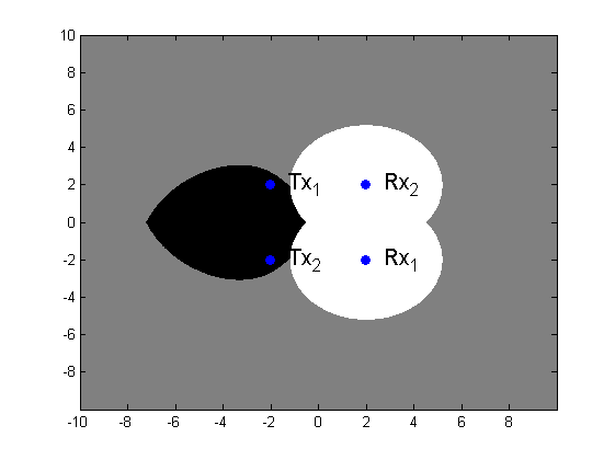
Figure 2: The geographical position in the 2D-plane in which the VSI conditions hold for the ICR subject to phase fading. The black region shows the location of the relay for ICRs without feedback in which DF at the relay achieves capacity at VSI. The union of the black and gray regions shows the location of the relay for ICRFs in which DF at the relay achieves capacity at VSI. The scenario parameters are detailed in Comment 6.

Comment 7.

Note from (4) that in the VSI regime, the ICRF behaves like two parallel relay channels.

Comment 8.

Although in practice there is only one relay node, it is simultaneously optimal for both “parallel relay channels” s.t. capacity is achieved in both simultaneously. From a practical aspect, this observation gives a strong motivation to employ a combination of relaying and feedback in wireless networks since a relatively small number of relay stations can optimally assist several nodes simultaneously.

Comment 9.

Note that since the capacity achieving channel inputs are mutually independent, adding relay nodes to the existing wireless networks does not require any modifications in the transmitters codebooks. Hence, these techniques (relaying with feedback) can be incorporated into current designs in a relatively simple manner.

Comment 10.

We now discuss the implication of having feedback of only channel outputs without CSI. Recall that in Comment 5 it is noted that, since feedback includes Rx-CSI as well as channel outputs, then, when feedback from both destinations to the relay is available, we can employ the DF scheme to obtain a characterization of the capacity region for any quality of links from the transmitters to the relay. When feedback does not include CSI from the receivers, then decoding the sources’ messages at the relay leads to additional restrictions on the channel coefficients, which are needed in order to arrive to a capacity characterization using DF. These restrictions decrease the set of channel coefficients for which the capacity region of the ICRF is achieved by the DF scheme. It should be emphasized that when the channel coefficients satisfy the additional restrictions, then the SI/VSI conditions are the same as those obtained with feedback that includes both Rx-CSI as well as channel output, and so are the rate constraints.

Comment 11.

Note that the capacity result in Theorem 1 holds also when there is no independent receiver at the relay, i.e., when $Y_{3}=\varnothing$, in the VSI regime. This observation holds only in scenarios where there are two noiseless feedback links, one from each receiver to the relay and not with partial feedback at the relay which will be studied in section VII. This is because the feedback turns each component relay channel into a degraded channel in the sense of [6]. In the next sections VI, VII, where we consider feedback to the transmitters and partial feedback, degradedness does not occur.

V ICRFs in the Strong Interference Regime

In this section, we characterize the capacity region of ICRFs in the SI regime. We consider two noiseless feedback links, one from each receiver to the relay. This capacity region is characterized in the following theorem:

Theorem 2.

Consider the fading ICRF with Rx-CSI. Assume that the channel coefficients are independent in time and independent of each other s.t. their phases are i.i.d. and distributed uniformly over $[0,2\pi)$. Let the additive noises be i.i.d. circularly symmetric complex Normal processes, $\mathcal{CN}(0,1)$, and let the sources have power constraints $\mathds{E}\big{\{}|X_{k}|^{2}\big{\}}\leq P_{k}$, $k\in\{1,2,3\}$. Assume noiseless feedback links from both receivers to the relay. If

$$I(X_{1},X_{3};Y_{1}|X_{2},\tilde{H}_{1}) \leq I(X_{1};Y_{2}|X_{2},\tilde{H}_{2})$$ (20a)

$$I(X_{2},X_{3};Y_{2}|X_{1},\tilde{H}_{2}) \leq I(X_{2};Y_{1}|X_{1},\tilde{H}_{1}),$$ (20b)

where the mutual information expressions are evaluated with $X_{k}\sim\mathcal{CN}(0,P_{k}),k\in\{1,2,3\}$, mutually independent, then the capacity region is given by all the nonnegative rate pairs s.t.

$$R_{1} \leq I(X_{1},X_{3};Y_{1}|X_{2},\tilde{H}_{1})$$ (21a)

$$R_{2} \leq I(X_{2},X_{3};Y_{2}|X_{1},\tilde{H}_{2})$$ (21b)

$$R_{1}+R_{2} \leq \min\big{\{}I(X_{1},X_{2},X_{3};Y_{1}|\tilde{H}_{1}),$$ (21c)

$$\qquad\;\;\;\;\;I(X_{1},X_{2},X_{3};Y_{2}|\tilde{H}_{2})\big{\}},$$

and it is achieved with $X_{k}\sim\mathcal{CN}(0,P_{k}),k\in\{1,2,3\}$, mutually independent and with DF strategy at the relay.

V-A Proof of Theorem 2

The proof consists of the following steps:

• From the ICRF we obtain the enhanced MARC (EMARC) as a MARC whose message destination is one of the destinations of the ICRF, but the relay receives feedback from both receivers. Therefore, EMARC₁ is defined by equations (1) and its receiver is Rx₁ and EMARC₂ is defined by equations (1) and its receiver is Rx₂.

• We derive the capacity region of EMARC₁ and EMARC₂.

• We show that the same coding strategy at the sources and at the relay achieves capacity for both EMARCs simultaneously.

  • We therefore obtain an achievable rate region for the ICRF as the intersection of capacity regions of EMARC₁ and EMARC₂.

• We show that in the SI regime the intersection of the capacity regions of EMARC₁ and EMARC₂ contains the capacity region of the ICRF .

• We characterize the SI conditions for the ICRF.

• We conclude the capacity region of ICRF in the SI regime is equal to the intersection of the capacity regions of EMARC₁ and EMARC₂.

The first three steps are detailed in section V-A1 and the last three steps are detailed in section V-A2.

V-A1 An Achievable Rate Region

Define $\underline{\mathbf{a}}\triangleq(a_{11},a_{21},a_{31},a_{12},a_{22},a_{32},a_{13},a_{23})$. Let $y_{1,1}^{i-1},y_{2,1}^{i-1},\tilde{h}_{1,1}^{i-1},\tilde{h}_{2,1}^{i-1}$ denote the available feedback at the relay at time $i$ in EMARC₁ and EMARC₂ and let $\mathcal{C}_{\scriptsize{\mbox{EMARC${}_{1}$}}}(\underline{\mathbf{a}})$ and $\mathcal{C}_{\scriptsize{\mbox{EMARC${}_{2}$}}}(\underline{\mathbf{a}})$ denote their capacity region, respectively. Let $t_{k}(R_{1},R_{2})$ denote the coding strategy (codebooks, encoders and decoders) for EMARC_k that achieves rate pair $(R_{1},R_{2})$. The capacity regions of the EMARCs are shown in Appendix B to be:

$$\!\!\!\!\!\!\!\!\!\!\!\!\mathcal{C}_{\scriptsize{\mbox{EMARC${}_{1}$}}}(\underline{\mathbf{a}})$$

$$\!\!\!\!\!\!\!\!=\bigg{\{}(R_{1},R_{2})\in\mathfrak{R}^{2}_{+}:$$

$$\;\;R_{1}\leq\min\big{\{}I(X_{1};Y_{1},Y_{2},Y_{3}|X_{2},X_{3},\underline{\tilde{H}}),$$

$$\qquad\qquad\qquad I(X_{1},X_{3};Y_{1}|X_{2},\tilde{H}_{1})\big{\}}$$ (22a)

$$\;\;R_{2}\leq\min\big{\{}I(X_{2};Y_{1},Y_{2},Y_{3}|X_{1},X_{3},\underline{\tilde{H}}),$$

$$\qquad\qquad\qquad I(X_{2},X_{3};Y_{1}|X_{1},\tilde{H}_{1})\big{\}}$$ (22b)

$$\;\;R_{1}+R_{2}\leq\min\big{\{}I(X_{1},X_{2};Y_{1},Y_{2},Y_{3}|X_{3},\underline{\tilde{H}}),$$

$$\qquad\qquad\qquad I(X_{1},X_{2},X_{3};Y_{1}|\tilde{H}_{1})\big{\}}\bigg{\}}$$ (22c)

$$\!\!\!\!\!\!\!\!\!\!\!\!\mathcal{C}_{\scriptsize{\mbox{EMARC${}_{2}$}}}(\underline{\mathbf{a}})$$

$$\!\!\!\!\!\!\!\!=\bigg{\{}(R_{1},R_{2})\in\mathfrak{R}^{2}_{+}:$$

$$\;\;R_{1}\leq\min\big{\{}I(X_{1};Y_{1},Y_{2},Y_{3}|X_{2},X_{3},\underline{\tilde{H}}),$$

$$\qquad\qquad\qquad I(X_{1},X_{3};Y_{2}|X_{2},\tilde{H}_{2})\big{\}}$$ (23a)

$$\;\;R_{2}\leq\min\big{\{}I(X_{2};Y_{1},Y_{2},Y_{3}|X_{1},X_{3},\underline{\tilde{H}}),$$

$$\qquad\qquad\qquad I(X_{2},X_{3};Y_{2}|X_{1},\tilde{H}_{2})\big{\}}$$ (23b)

$$\;\;R_{1}+R_{2}\leq\min\big{\{}I(X_{1},X_{2};Y_{1},Y_{2},Y_{3}|X_{3},\underline{\tilde{H}}),$$

$$\qquad\qquad\qquad I(X_{1},X_{2},X_{3};Y_{2}|\tilde{H}_{2})\big{\}}\bigg{\}},$$ (23c)

where $X_{k}\sim\mathcal{CN}(0,P_{k}),k\in\{1,2,3\}$ are mutually independent and DF is used at the relay.

Next, we have the following proposition:

Proposition 1.

The same coding strategy at the sources and at the relay achieves capacity for both EMARCs simultaneously, i.e.,

$$\mathcal{C}_{\scriptsize{\mbox{EMARC${}_{1}$}}}(\underline{\mathbf{a}})\cap\mathcal{C}_{\scriptsize{\mbox{EMARC${}_{2}$}}}(\underline{\mathbf{a}})\subseteq\mathcal{C}_{ICRF}(\underline{\mathbf{a}}).$$ (24)

Proof.

In Appendix B it is shown that the capacity region of each EMARC is achieved with DF strategy at the relay and codebooks generated according to independent circularly symmetric complex Normal distribution at the sources and at the relay (the same distributions are used in both EMARCs). In both EMARCs, for all rate pairs $(R_{1},R_{2})$, the relay codebook has $2^{n(R_{1}+R_{2})}$ codewords generated i.i.d. according to $\mathcal{CN}(0,P_{3})$, independent of the codewords at the sources. For all rate pairs $(R_{1},R_{2})$ the same scheme is used at the relay in both EMARCs: at block $b$ the relay decodes the messages $(m_{1,b},m_{2,b})$ via a joint-typicality decoder using $\big{(}\mathbf{y}_{1}(b),\mathbf{y}_{2}(b),\mathbf{y}_{3}(b),\mathbf{\underline{\tilde{h}}}(b)\big{)}$, and transmits $\mathbf{x}_{3}(m_{1,b},m_{2,b})$. Thus, all rate pairs $(R_{1},R_{2})$ s.t. $(R_{1},R_{2})\in\mathcal{C}_{\scriptsize{\mbox{EMARC${}_{1}$}}}(\underline{\mathbf{a}})\cap\mathcal{C}_{\scriptsize{\mbox{EMARC${}_{2}$}}}(\underline{\mathbf{a}})$ are achieved at both EMARCs simultaneously with $t_{1}(R_{1},R_{2})=t_{2}(R_{1},R_{2})=t_{DF}(R_{1},R_{2})$, where $t_{DF}(R_{1},R_{2})$ is the coding strategy detailed in Appendix B, for achieving the rate pair $(R_{1},R_{2})$. ∎

From Proposition 1 it follows that an achievable rate region for the ICRF, $\mathcal{R}_{\scriptsize{ICRF}}(\underline{\mathbf{a}},t_{DF})$ (here $t_{DF}$ should be understood as the DF strategy appropriate for each rate pair in the achievable region, see Appendix B), can be obtained by:

$$\!\!\!\!\!\!\!\mathcal{R}_{\scriptsize{ICRF}}(\underline{\mathbf{a}},t_{DF})$$

$$\quad=\mathcal{C}_{\scriptsize{\mbox{EMARC${}_{1}$}}}(\underline{\mathbf{a}})\cap\mathcal{C}_{\scriptsize{\mbox{EMARC${}_{2}$}}}(\underline{\mathbf{a}})\subseteq\mathcal{C}_{\scriptsize{\mbox{ICRF}}}(\underline{\mathbf{a}}),$$ (25)

and it is achieved with $X_{k}\sim\mathcal{CN}(0,P_{k}),k\in\{1,2,3\}$, independent of each other and with DF strategy at the relay.

V-A2 Converse

By definition of the SI regime, in this regime both receivers can decode both messages without reducing the capacity region, i.e., any achievable rate pair $(R_{1},R_{2})\in\mathcal{C}_{\scriptsize{\mbox{ICRF}}}(\underline{\mathbf{a}})$ is also achievable in EMARC₁ and EMARC₂, hence $\mathcal{C}_{\scriptsize{\mbox{ICRF}}}(\underline{\mathbf{a}})\subseteq\mathcal{C}_{\scriptsize{\mbox{EMARC${}_{1}$}}}(\underline{\mathbf{a}})\cap\mathcal{C}_{\scriptsize{\mbox{EMARC${}_{2}$}}}(\underline{\mathbf{a}})$. Combined with equation (V-A1) we conclude that in the SI regime $\mathcal{C}_{\scriptsize{\mbox{ICRF}}}(\underline{\mathbf{a}})=\mathcal{C}_{\scriptsize{\mbox{EMARC${}_{1}$}}}(\underline{\mathbf{a}})\cap\mathcal{C}_{\scriptsize{\mbox{EMARC${}_{2}$}}}(\underline{\mathbf{a}})$. Hence, the only problem left open is to determine the SI conditions for the ICRF. Note that from proposition 1 we obtain that $\mathcal{C}_{\scriptsize{\mbox{EMARC${}_{1}$}}}(\underline{\mathbf{a}})$ and $\mathcal{C}_{\scriptsize{\mbox{EMARC${}_{2}$}}}(\underline{\mathbf{a}})$ are achieved with $t_{DF}$, thus for the rest of the proof we only consider mutually independent, circularly symmetric complex Normal channel inputs with zero mean. The rest of the proof consists of the following steps:

• We assume an achievable rate pair $(R_{1},R_{2})$ in the ICRF.

• We characterize the maximal rate at which each receiver can decode its desired message. We conclude that this rate is achieved with independent channel inputs generated i.i.d. according to the circularly symmetric complex Normal distribution (see Theorem B.1 in Appendix B).

• We characterize the worst case conditions for each receiver to decode the interfering message.

• We derive the conditions for which decoding both messages at each receiver does not reduce the capacity region.

For the first two steps note that the maximal rates for decoding at the destinations are given by the cut-set bounds in (5), i.e.,

$$\mbox{max }R_{1} = \!\!\!\!\!\!\!\!\sup_{f(x_{1},x_{2},x_{3})}\Big{\{}\min\big{\{}I(X_{1};Y_{1},Y_{2},Y_{3}|X_{2},X_{3},\underline{\tilde{H}}),$$ (26a)

$$\qquad\qquad I(X_{1},X_{3};Y_{1}|X_{2},\tilde{H}_{1})\big{\}}\Big{\}}$$

$$\mbox{max }R_{2} = \!\!\!\!\!\!\!\!\sup_{f(x_{1},x_{2},x_{3})}\Big{\{}\min\big{\{}I(X_{2};Y_{1},Y_{2},Y_{3}|X_{1},X_{3},\underline{\tilde{H}}),$$ (26b)

$$\qquad\qquad I(X_{2},X_{3};Y_{2}|X_{1},\tilde{H}_{2})\big{\}}\Big{\}},$$

and they are achieved with mutually independent, circularly symmetric complex Normal channel inputs with zero mean and with DF at the relay (see Appendix B for a detailed proof). The worst case scenario for decoding at the destinations, however, is when the signal from the relay degrades the performance of the receivers. Given two vectors, $\mathbf{a}$ and $\mathbf{b}$, define the notation $\mathbf{a}\cdot\mathbf{b}\triangleq(a_{1}b_{1},a_{2}b_{2},...,a_{n}b_{n})$. Assume the rate pair $(R_{1},R_{2})\in\mathcal{C}_{\scriptsize{\mbox{ICRF}}}(\underline{\mathbf{a}})$. If Rx₁ can decode $m_{1}$ from the signal

$$\mathbf{y}_{1}=\mathbf{h}_{11}\cdot\mathbf{x}_{1}+\mathbf{h}_{21}\cdot\mathbf{x}_{2}+\mathbf{h}_{31}\cdot\mathbf{x}_{3}+\mathbf{z}_{1},$$

then it can create the signal

$$\mathbf{y}_{1}^{\prime}=\mathbf{h}_{21}\cdot\mathbf{x}_{2}+\mathbf{h}_{31}\cdot\mathbf{x}_{3}+\mathbf{z}_{1},$$

from which it can decode $m_{2}$ by treating $\mathbf{h}_{31}\cdot\mathbf{x}_{3}$ as additive noise if

$$R_{2}\leq I(X_{2};Y_{1}^{\prime}|\tilde{H}_{1})\triangleq R_{2}^{\prime}.$$

Similarly, Rx₂ can decode $m_{1}$ if

$$R_{1}\leq I(X_{1};Y_{2}^{\prime}|\tilde{H}_{2})\triangleq R_{1}^{\prime}.$$

Next, we should guarantee that decoding both messages at each receiver does not reduce the capacity region of the ICRF. This is achieved if $\max R_{1}\leq R_{1}^{\prime}$ and $\max R_{2}\leq R_{2}^{\prime}$, i.e.,

$$\!\!\!\!\!\!\!\!\!\!\!\!\!\!\!\sup_{f(x_{1},x_{2},x_{3})}\Big{\{}\min\big{\{}I(X_{1};Y_{1},Y_{2},Y_{3}|X_{2},X_{3},\underline{\tilde{H}}),$$

$$\qquad\qquad\qquad\qquad I(X_{1},X_{3};Y_{1}|X_{2},\tilde{H}_{1})\big{\}}\Big{\}}$$

$$\leq I(X_{1};Y_{2}^{\prime}|\tilde{H}_{2})$$

$$\stackrel{{\scriptstyle(a)}}{{=}}I(X_{1};Y_{2}|X_{2},\tilde{H}_{2}),$$

$$\!\!\!\!\!\!\!\!\!\!\!\!\!\!\!\sup_{f(x_{1},x_{2},x_{3})}\Big{\{}\min\big{\{}I(X_{2};Y_{1},Y_{2},Y_{3}|X_{1},X_{3},\underline{\tilde{H}}),$$

$$\qquad\qquad\qquad\qquad I(X_{2},X_{3};Y_{2}|X_{1},\tilde{H}_{2})\big{\}}\Big{\}}$$

$$\leq I(X_{2};Y_{1}^{\prime}|\tilde{H}_{1})$$

$$=I(X_{2};Y_{1}|X_{1},\tilde{H}_{1}),$$

where (a) follows from the fact that the capacity region of the ICRF in the SI regime, as well as the supremum on the left-hand side (l.h.s.) of the inequality, are achieved with $X_{k}\sim\mathcal{CN}(0,P_{k}),k\in\{1,2,3\}$, independent of each other and of the channel coefficients; thus all mutual information expressions are evaluated with the same distribution. Note that from arguments similar to those used in section IV-A3, we also obtain that

$$I(X_{1};Y_{2}|X_{2},\tilde{H}_{2}) \leq I(X_{1};Y_{1},Y_{2},Y_{3}|X_{2},X_{3},\underline{\tilde{H}})$$

$$I(X_{2};Y_{1}|X_{1},\tilde{H}_{1}) \leq I(X_{2};Y_{1},Y_{2},Y_{3}|X_{1},X_{3},\underline{\tilde{H}}).$$

Thus, to guarantee that $\max R_{1}\leq R_{1}^{\prime}$ and $\max R_{2}\leq R_{2}^{\prime}$, it is enough to require

$$I(X_{1},X_{3};Y_{1}|X_{2},\tilde{H}_{1}) \leq I(X_{1};Y_{2}|X_{2},\tilde{H}_{2})$$ (27a)

$$I(X_{2},X_{3};Y_{2}|X_{1},\tilde{H}_{2}) \leq I(X_{2};Y_{1}|X_{1},\tilde{H}_{1}),$$ (27b)

which give (20). Hence, when (27) holds, $\mathcal{C}_{\scriptsize{\mbox{ICRF}}}(\underline{\mathbf{a}})=\mathcal{C}_{\scriptsize{\mbox{EMARC${}_{1}$}}}(\underline{\mathbf{a}}_{1})\cap\mathcal{C}_{\scriptsize{\mbox{EMARC${}_{2}$}}}(\underline{\mathbf{a}}_{2})$.

Comment 12.

Note that the argument presented here uses only local Rx-CSI, as opposed to the argument of Sato [3].

V-A3 Simplification of the Capacity Region

Consider the constraints on $R_{1}$ in (22) and (23). Note that if (27) holds, since the channel inputs are independent of each other and of the channel coefficients, we get

$$I(X_{1},X_{3};Y_{1}|X_{2},\tilde{H}_{1}) \leq I(X_{1};Y_{2}|X_{2},\tilde{H}_{2})$$

$$\leq I(X_{1},X_{3};Y_{2}|X_{2},\tilde{H}_{2}),$$

$$I(X_{1},X_{3};Y_{1}|X_{2},\tilde{H}_{1}) \leq I(X_{1};Y_{2}|X_{2},\tilde{H}_{2})$$

$$\leq I(X_{1};Y_{1},Y_{2},Y_{3}|X_{2},X_{3},\underline{\tilde{H}}).$$

Thus, the constraints on $R_{1}$ in (22) and (23) can be reduced to

$$R_{1}\leq I(X_{1},X_{3};Y_{1}|X_{2},\tilde{H}_{1}).$$ (28a)

Following the same steps, the constraints on $$R_{2}$$ in (22) and (23) can be reduced to

$$R_{2}\leq I(X_{2},X_{3};Y_{2}|X_{1},\tilde{H}_{2}).$$ (28b)

Finally, note that since the channel inputs are independent of each other and of the channel coefficients, then

$$I(X_{1};Y_{2}|\tilde{H}_{1}) \leq I(X_{1};Y_{2}|X_{2},\underline{\tilde{H}})$$

$$\leq I(X_{1};Y_{1},Y_{2},Y_{3}|X_{2},X_{3},\underline{\tilde{H}})$$

$$I(X_{2};Y_{1}|\tilde{H}_{1}) \leq I(X_{2};Y_{1},Y_{2},Y_{3}|X_{3},\underline{\tilde{H}}).$$

Hence, when (27) is satisfied,

$$\!\!\!\!\!\!\!\!\!\!\!\!\!\!\!\!\!\!\!\!\!\!\!\!\!I(X_{1},X_{2};Y_{1},Y_{2},Y_{3}|X_{3},\underline{\tilde{H}})$$

$$= I(X_{2};Y_{1},Y_{2},Y_{3}|X_{3},\underline{\tilde{H}})$$

$$\qquad+I(X_{1};Y_{1},Y_{2},Y_{3}|X_{2},X_{3},\underline{\tilde{H}})$$

$$\geq I(X_{2};Y_{1}|\tilde{H}_{1})+I(X_{1},X_{3};Y_{1}|X_{2},\tilde{H}_{1})$$

$$= I(X_{1},X_{2},X_{3};Y_{1}|\tilde{H}_{1}),$$

and

$$I(X_{1},X_{2};Y_{1},Y_{2},Y_{3}|X_{3},\underline{\tilde{H}})\geq I(X_{1},X_{2},X_{3};Y_{2}|\tilde{H}_{2}),$$

implying that in the SI regime, the sum-rate conditions for decoding at the relay is always satisfied. This shows that when (20) holds, the capacity region is characterized in (21).

$\blacksquare$

V-B Ergodic Phase Fading

When the channel is subject to ergodic phase fading, we obtain the following explicit result:

Corollary 3.

Consider the phase fading ICRF with Rx-CSI and noiseless feedback links from both receivers to the relay, s.t. $y_{1,1}^{i-1},y_{2,1}^{i-1},\tilde{h}_{1,1}^{i-1}$ and $\tilde{h}_{2,1}^{i-1}$ are available at the relay at time $i$. If the channel coefficients satisfy

$$a_{11}^{2}P_{1}+a_{31}^{2}P_{3} \leq \frac{a_{12}^{2}P_{1}}{1+a_{32}^{2}P_{3}}$$ (29a)

$$a_{22}^{2}P_{2}+a_{32}^{2}P_{3} \leq \frac{a_{21}^{2}P_{2}}{1+a_{31}^{2}P_{3}},$$ (29b)

then the capacity region is characterized by all the nonnegative rate pairs s.t.

$$R_{1} \leq \log_{2}\big{(}1+a_{11}^{2}P_{1}+a_{31}^{2}P_{3}\big{)}$$ (30a)

$$R_{2} \leq \log_{2}\big{(}1+a_{22}^{2}P_{2}+a_{32}^{2}P_{3}\big{)}$$ (30b)

$$R_{1}+R_{2} \leq \min\bigg{\{}\log_{2}(1+a_{11}^{2}P_{1}+a_{21}^{2}P_{2}+a_{31}^{2}P_{3}),$$ (30c)

$$\log_{2}(1+a_{12}^{2}P_{1}+a_{22}^{2}P_{2}+a_{32}^{2}P_{3})\bigg{\}},$$

and it is achieved with $X_{k}\sim\mathcal{CN}(0,P_{k}),k\in\{1,2,3\}$, mutually independent and with DF strategy at the relay.

Proof.

The result follows from the expressions of Theorem 2. In order to obtain the conditions on the channel coefficients in (29) we first evaluate $I(X_{1},X_{3};Y_{1}|X_{2},\tilde{H}_{1})$ and $I(X_{2},X_{3};Y_{2}|X_{1},\tilde{H}_{2})$ as in Corollary 1, by using the r.h.s. of (A-A). Also note that $\{H_{31,i}X_{3,i}\}_{i=1}^{n}$ can be considered as additive Gaussian noise at Rx₁ and $\{H_{32,i}X_{3,i}\}_{i=1}^{n}$ can be considered as additive Gaussian noise at Rx₂. Therefore from the independence of the channel inputs we obtain

$$I(X_{2};Y_{1}|X_{1},\tilde{H}_{1}) = \log_{2}\Big{(}1+\frac{a_{21}^{2}P_{2}}{1+a_{31}^{2}P_{3}}\Big{)}$$

$$I(X_{1};Y_{2}|X_{2},\tilde{H}_{2}) = \log_{2}\Big{(}1+\frac{a_{12}^{2}P_{1}}{1+a_{32}^{2}P_{3}}\Big{)}.$$

Thus, by evaluating (20) we obtain the conditions in (29). Finally, we evaluate $I(X_{1},X_{2},X_{3};Y_{1}|\tilde{H}_{1})$ and $I(X_{1},X_{2},X_{3};Y_{2}|\tilde{H}_{2})$ by using the r.h.s. of (B-A):

$$I(X_{1},X_{2},X_{3};Y_{1}|\tilde{H}_{1})$$

$$\qquad\qquad\qquad=\log_{2}(1+a_{11}^{2}P_{1}+a_{21}^{2}P_{2}+a_{31}^{2}P_{3})$$

$$I(X_{1},X_{2},X_{3};Y_{2}|\tilde{H}_{2})$$

$$\qquad\qquad\qquad=\log_{2}(1+a_{12}^{2}P_{1}+a_{22}^{2}P_{2}+a_{32}^{2}P_{3}).$$

∎

V-C Ergodic Rayleigh Fading

Define $\tilde{U}_{k}\triangleq(U_{kk},U_{3k}),k\in\{1,2\}$ and $\underline{\tilde{U}}\triangleq(U_{11},U_{12},U_{21},U_{22},U_{31},U_{32})$. When the channel is subject to ergodic Rayleigh fading, we obtain the following explicit result:

Corollary 4.

Consider the Rayleigh fading ICRF with Rx-CSI and noiseless feedback links from both receivers to the relay, s.t. $y_{1,1}^{i-1},y_{2,1}^{i-1},\tilde{h}_{1,1}^{i-1}$ and $\tilde{h}_{2,1}^{i-1}$ are available at the relay at time $i$. If the channel coefficients satisfy

$$\!\!\!\!\!\!\!\!\!\!\!\!\frac{\frac{a_{12}^{2}P_{1}}{1+a_{32}^{2}P_{3}}}{e^{\frac{1+a_{32}^{2}P_{3}}{a_{12}^{2}P_{1}}}E_{1}\left(\frac{1+a_{32}^{2}P_{3}}{a_{12}^{2}P_{1}}\right)} \geq (1+a_{11}^{2}P_{1}+a_{31}^{2}P_{3})$$ (31a)

$$\!\!\!\!\!\!\!\!\!\!\!\!\frac{\frac{a_{21}^{2}P_{2}}{1+a_{31}^{2}P_{3}}}{e^{\frac{1+a_{31}^{2}P_{3}}{a_{21}^{2}P_{2}}}E_{1}\left(\frac{1+a_{31}^{2}P_{3}}{a_{21}^{2}P_{2}}\right)} \geq (1+a_{22}^{2}P_{2}+a_{32}^{2}P_{3}),$$ (31b)

then the capacity region is characterized by all the nonnegative rate pairs s.t.

$$\!\!\!\!\!\!\!\!\!\!\!\!\!\!\!\!R_{1}\leq\mathds{E}_{\tilde{U}_{1}}\!\big{\{}\log_{2}(1+a_{11}^{2}|U_{11}|^{2}P_{1}+a_{31}^{2}|U_{31}|^{2}P_{3})\big{\}}$$ (32a)

$$\!\!\!\!\!\!\!\!\!\!\!\!\!\!\!\!R_{2}\leq\mathds{E}_{\tilde{U}_{2}}\!\big{\{}\log_{2}(1+a_{22}^{2}|U_{22}|^{2}P_{2}+a_{32}^{2}|U_{32}|^{2}P_{3})\big{\}}$$ (32b)

$$\!\!\!\!\!\!\!\!\!\!\!\!\!\!\!\!R_{1}+R_{2}\leq\min_{k\in\{1,2\}}\Big{\{}\mathds{E}_{\underline{\tilde{U}}}\!\big{\{}\log_{2}(1+a_{1k}^{2}|U_{1k}|^{2}P_{1}$$

$$\qquad\qquad+a_{2k}^{2}|U_{2k}|^{2}P_{2}+a_{3k}^{2}|U_{3k}|^{2}P_{3})\big{\}}\Big{\}},$$ (32c)

and it is achieved with $X_{k}\sim\mathcal{CN}(0,P_{k}),k\in\{1,2,3\}$, mutually independent and with DF strategy at the relay.

Proof.

The result follows from the expressions of Theorem 2 and follows the same approach as in the proof of Corollary 3. Here (31) follows from [18, Proposition 1]. ∎

(a) The range of $a_{12}$ and $a_{21}$ which satisfy the conditions for the VSI regime (gray area only) and for the SI regime (both black and gray areas) when DF achieves capacity in the phase fading scenario.

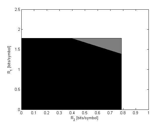
(b) The capacity region of the ICRF for the phase fading scenario in the VSI regime (both black and gray areas, $a_{12}=a_{21}=0.7$) and the SI regime (black area only, $a_{12}=0.53$, $a_{21}=0.36$)

Figure 3: SI and VSI for $P_{1}=P_{2}=P_{3}=10,a_{11}=0.42,a_{22}=0.25,a_{31}=0.26$ and $a_{32}=0.1.$

V-D Comments

Comment 13.

In order to compare the feedback capacity region of Corollary 3 to that obtained without feedback, let $\mathcal{D}_{k}$ be the set of channel coefficients $\mathbf{a}_{k}=\big{(}a_{1k},a_{2k},a_{3k},a_{13},a_{23}\big{)}\in\mathfrak{R}^{5}_{+}$ that satisfy

$$a_{1k}^{2}P_{1}+a_{3k}^{2}P_{3} \leq a_{13}^{2}P_{1}$$ (33a)

$$a_{2k}^{2}P_{2}+a_{3k}^{2}P_{3} \leq a_{23}^{2}P_{2}$$ (33b)

$$a_{1k}^{2}P_{1}+a_{2k}^{2}P_{2}+a_{3k}^{2}P_{3} \leq a_{13}^{2}P_{1}+a_{23}^{2}P_{2},$$ (33c)

$k=1,2$. Let $\mathbf{a}\triangleq\big{(}a_{11},a_{12},a_{13},a_{21},a_{22},a_{23},a_{31},a_{32}\big{)}\in\mathfrak{R}^{8}_{+}$ and let $\mathbf{a}\in\mathcal{D}_{1}\cap\mathcal{D}_{2}$ be a short form notation to denote that $\mathbf{a}_{1}$ and $\mathbf{a}_{2}$ satisfy $\big{\{}\mathbf{a}_{1}\cup\mathbf{a}_{2}=\mathbf{a}\big{\}}\bigcap\big{\{}\mathbf{a}_{1}\in\mathcal{D}_{1}\big{\}}\bigcap\big{\{}\mathbf{a}_{2}\in\mathcal{D}_{2}\big{\}}$.

[17, Theorem 2] states that when the channel coefficients satisfy (29) and also $\mathbf{a}\in\mathcal{D}_{1}\cap\mathcal{D}_{2}$, then the capacity region is given by (30). Similar to VSI (see Comment 5), observe that the rate constraints are the same for both the feedback and the no-feedback cases, thus when capacity is achieved without feedback, then feedback does not enlarge the capacity region. Using similar arguments as in the discussion in Comment 5, it is possible to show that when (29) hold, then there are situations in which feedback enlarges the capacity region. The same conclusion applies to Rayleigh fading as well.

Comment 14.

Since the optimal codewords are generated independent of each other and of the channel coefficients, we obtain

$$I(X_{1};Y_{2}|\tilde{H}_{2}) \leq I(X_{1};Y_{2}|X_{2},\tilde{H}_{2})$$

$$I(X_{2};Y_{1}|\tilde{H}_{1}) \leq I(X_{2};Y_{1}|X_{1},\tilde{H}_{1}),$$

thus, its easy to see that the SI conditions in (20) are weaker than the VSI conditions in (3), as depicted in Fig. 3a. The capacity region are compared in Fig. 3b.

Comment 15.

Although in the SI regime the resulting model can be thought of as a “compound EMARC”, it is important to note that both EMARCs share the same relay and thus they are not separate, contrary to ICs without relay. Note that the strategy at the relay is optimal for both EMARCs s.t. capacity is achieved for both simultaneously.

VI ICRs with Feedback to the Relay and Transmitters

In this section we study the scenarios in which feedback is available both at the relay and at the transmitters. We consider two configurations: (1) feedback from each receiver to the relay and to its opposite transmitter, (2) feedback from each receiver to the relay and to its corresponding transmitter.

VI-A Feedback to the Opposite Transmitters

First, we study how the capacity region is affected if there are two noiseless feedback links from each receiver, both to the relay and to its opposite transmitter, s.t. $y_{1,1}^{i-1},\tilde{h}_{1,1}^{i-1}$ are available at Tx₂, $y_{2,1}^{i-1},\tilde{h}_{2,1}^{i-1}$ are available at Tx₁, and $y_{1,1}^{i-1},y_{2,1}^{i-1},\tilde{h}_{1,1}^{i-1},\tilde{h}_{2,1}^{i-1}$ are available at the relay at time $i$, prior to the transmission at each node. for this scenario, the definitions of the encoders at the transmitters in Definition 1 are modified as follows:

$$x_{1,i} = e_{1,i}(m_{1},y_{2,1}^{i-1},\tilde{h}_{2,1}^{i-1})$$ (34a)

$$x_{2,i} = e_{2,i}(m_{2},y_{1,1}^{i-1},\tilde{h}_{1,1}^{i-1});$$ (34b)

the rest of the definitions remain unchanged and they are the same as in section II. This model can represent scenarios where each transmitter is close to its opposite receiver, e.g., when VSI occurs in the ICRF. This configuration is depicted in Fig. 4.

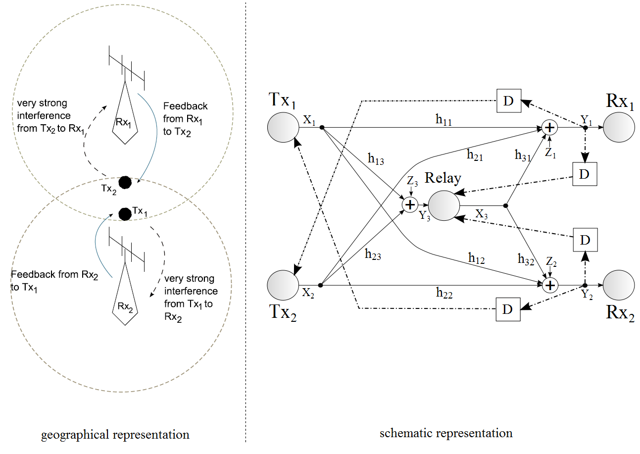
Figure 4: The interference channel with a relay and feedback from both receivers to the relay and to their opposite transmitters. The ‘D’ block represents a single-symbol delay.

Proposition 2.

Consider the ICRF in which there is a noiseless feedback link from each receiver to the relay. Then, additional feedback links from each receiver to its opposite transmitter (see Fig. 4), do not provide any further enlargement to the capacity region in the VSI regime.

Proof.

Let $m_{1}\in\mathcal{M}_{1},m_{2}\in\mathcal{M}_{2}$ denote the messages that Tx₁ and Tx₂ send to Rx₁ and Rx₂, respectively. Let the encoders at Tx₁ and Tx₂ map their messages and the information received from their feedback links into the channel input symbols $x_{1,i}$ and $x_{2,i}$, respectively. Thus, the encoders at the transmitters are given in (34). The encoder at the relay remains unchanged, i.e., it is the causal function given in (2). Consider the cut-set bound expressions in (5). Observe that in the cut-set bounds on $R_{1}$, Rx₁ and Tx₂ belong to $\mathcal{S}^{C}$ while Tx₁ and Rx₂ belong to $\mathcal{S}$. Hence, by inspection of the proof of the cut-set bound [39, Theorem 15.10.1], it is evident that the encoders at Tx₁ and Tx₂ used for the cut-set expressions are exactly those in (34) and therefore the cut-set expressions for rates $R_{1}$ and $R_{2}$ in (5) remain unchanged when feedback is also sent from each receiver to its opposite transmitter.

Finally, note that Theorem 1 proves that in the VSI regime, if feedback from both receivers is available at the relay then the cut-set bounds (5b) and (5d) are achievable and there is no constraint on the sum-rate. Hence, we conclude that when feedback from both receivers is available at the relay then additional feedback links from each receiver to its opposite transmitter do not enlarge the capacity region of the ICRF in the VSI regime. ∎

VI-A1 Comments

Comment 16.

In [20] it was shown that feedback can increase the capacity region of the discrete memoryless MAC by allowing the sources to coordinate their transmissions. In the ICRF with additional feedback links from each receiver to its opposite transmitter, since the cut-set bound expressions are maximized with mutually independent channel inputs then such coordination is not beneficial and in fact it is not possible.

Comment 17.

We conclude that if, due network limitations, each receiver may send feedback either to the relay or to its opposite transmitter (when in the VSI regime (3)), then its preferable to send feedback to the relay, since the relay can exploit the additional information to achieve the capacity in the VSI regime.

VI-B Feedback to the Corresponding Transmitters

In this section, we study how the capacity region is affected if there are two noiseless feedback links from each receiver, both to the relay and to its corresponding transmitter, s.t. $y_{1,1}^{i-1},\tilde{h}_{1,1}^{i-1}$ are available at Tx₁, $y_{2,1}^{i-1},\tilde{h}_{2,1}^{i-1}$ are available at Tx₂, and $y_{1,1}^{i-1},y_{2,1}^{i-1},\tilde{h}_{1,1}^{i-1},\tilde{h}_{2,1}^{i-1}$ are available at the relay, at time $i$, prior to the transmission at each node. For this scenario the encoders at the transmitters in Definition 1 are changed to

$$x_{1,i} = e_{1,i}(m_{1},y_{1,1}^{i-1},\tilde{h}_{1,1}^{i-1})$$ (35a)

$$x_{2,i} = e_{2,i}(m_{2},y_{2,1}^{i-1},\tilde{h}_{2,1}^{i-1}),$$ (35b)

the rest of the definitions are the same as in section II. This configuration is depicted in Fig. 5.

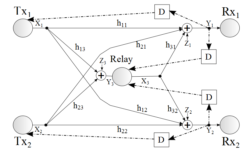
Figure 5: The interference channel with a relay and feedback from both receivers to the relay and to their corresponding transmitters. The ‘D’ block represents a single-symbol delay.

Let $\tilde{\mathcal{C}}_{MAC-FB}$ and $\tilde{\mathcal{R}}_{OB}$ be defined as

$$\!\!\!\!\!\!\!\!\!\!\!\!\!\!\!\!\tilde{\mathcal{C}}_{MAC-FB}$$

$$\!\!\!\!\!\!\!\!\!\!\!\!\triangleq\bigg{\{}(R_{1},R_{2})\in\mathfrak{R}_{+}^{2}:$$

$$R_{1}\leq I(X_{1};Y_{1},Y_{2},Y_{3}|X_{2},X_{3},\underline{\tilde{H}})$$ (36a)

$$R_{2}\leq I(X_{2};Y_{1},Y_{2},Y_{3}|X_{1},X_{3},\underline{\tilde{H}})$$ (36b)

$$R_{1}+R_{2}\leq I(X_{1},X_{2};Y_{1},Y_{2},Y_{3}|X_{3},\underline{\tilde{H}})\;\bigg{\}},$$ (36c)

$$\!\!\!\!\!\!\!\!\!\!\!\!\!\!\!\!\tilde{\mathcal{R}}_{OB}$$

$$\!\!\!\!\!\!\!\!\!\!\!\!\triangleq\bigg{\{}(R_{1},R_{2})\in\mathfrak{R}_{+}^{2}:$$

$$R_{1}\leq I(X_{1},X_{3};Y_{1},Y_{2}|X_{2},\underline{\tilde{H}})$$ (37a)

$$R_{2}\leq I(X_{2},X_{3};Y_{1},Y_{2}|X_{1},\underline{\tilde{H}})$$ (37b)

$$R_{1}+R_{2}\leq I(X_{1},X_{2},X_{3};Y_{1},Y_{2}|\underline{\tilde{H}})\quad\bigg{\}},$$ (37c)

where all mutual information expressions in (36) and (37) are evaluated with $X_{k}\sim\mathcal{CN}(0,P_{k})$, $k=1,2,3$, mutually independent. Next, define the region $\tilde{\mathcal{R}}_{ICRF}^{VSI}$ as follows:

$$\!\!\!\!\!\!\!\!\!\!\!\!\!\!\!\!\tilde{\mathcal{R}}_{ICRF}^{VSI}$$

$$\!\!\!\!\!\!\!\!\!\!\!\!\!\!\!\!\!\!\!\triangleq\bigg{\{}(R_{1},R_{2})\in\mathfrak{R}_{+}^{2}:$$

$$R_{2}\leq I(X_{2},X_{3};Y_{2}|X_{1},\tilde{H}_{2})$$

$$R_{1}\leq I(X_{1},X_{2},X_{3};Y_{1}|\tilde{H}_{1})$$

$$\qquad\qquad-\frac{I(X_{2};Y_{1}|\tilde{H}_{1})}{I(X_{2},X_{3};Y_{2}|X_{1},\tilde{H}_{2})}R_{2}\bigg{\}},$$

where all mutual information expression are evaluated with $X_{k}\sim\mathcal{CN}(0,P_{k})$, $k=1,2,3$, mutually independent. We now state the inner and outer bound in the following proposition:

Proposition 3.

The capacity region of the ICRF with noiseless feedback links from each receiver to the relay and to its corresponding transmitter, denoted $\tilde{\mathcal{C}}_{ICRF}$, is outer bounded by $\tilde{\mathcal{C}}_{ICRF}\subseteq\tilde{\mathcal{C}}_{MAC-FB}\cap\tilde{\mathcal{R}}_{OB}$. Furthermore, if the VSI conditions (3) hold and also

$$I(X_{1},X_{2},X_{3};Y_{1}|\tilde{H}_{1})\leq I(X_{1};Y_{2}|X_{2},X_{3},\tilde{H}_{2}),$$ (38)

holds for mutually independent Gaussian inputs, $X_{k}\sim\mathcal{CN}(0,P_{k})$, $k=1,2,3$. Then, the corresponding capacity region of the ICRF in the VSI regime, denoted $\tilde{\mathcal{C}}_{ICRF}^{VSI}$, satisfies $\tilde{\mathcal{C}}_{ICRF}^{VSI}\supseteq\tilde{\mathcal{R}}_{ICRF}^{VSI}$.

Proof.

See Appendix C. ∎

As a direct consequence of Proposition 3 we have the following corollary:

Corollary 5.

Consider the ICRF with two noiseless feedback links from the receivers to the relay. Then, additional feedback links from each receiver to its corresponding transmitter (see Fig. 5), enlarge the capacity region in the SI and VSI regimes.

VI-B1 Comments

Comment 18.

Note that feedback to the corresponding transmitters also increases the capacity region of the ICRF in the SI regime. The proof is identical to the one used in Proposition 3 subject to (38) and conditions (20). In particular, the outer bound is identical to that in the proof of Proposition 3, and the achievable rate region is obtained by time sharing between $\big{(}I(X_{1},X_{2},X_{3};Y_{1}|\tilde{H}_{1}),0\big{)}$ and the rate points of the SI region (21).

Comment 19.

Note that in the coding scheme described in Proposition 3, Tx₂ behaves like a second relay node for Tx₁, i.e., the ICRF is transformed into a multiple relay channel. It should also be noted that when $\mbox{Tx}_{2}$ cooperates with $\mbox{Tx}_{1}$ and with the relay in sending $m_{1}$, this decreases the maximal rate of information that could be sent from $\mbox{Tx}_{2}$ to $\mbox{Rx}_{2}$. However, as this cooperation increases the maximal achievable rate from $\mbox{Tx}_{1}$ to $\mbox{Rx}_{1}$, compared to the case where feedback is available only at the relay, the capacity region is increased.

Comment 20.

Recall that in the classic relay channel Rx-Tx feedback does not enlarge the capacity region once feedback from the receiver is available at the relay node. In ICRF, in contrary to the classic relay channel, Rx-Tx feedback can enlarge the capacity region beyond what is achieved with Rx-relay feedback. Thus, not all of the insights from the study of the classic relay channel hold for the ICRF.

Comment 21.

The boundaries of $\tilde{\mathcal{R}}_{ICRF}^{VSI}$ and $\tilde{\mathcal{C}}_{MAC-FB}\cap\tilde{\mathcal{R}}_{OB}$, together with the capacity region of the ICRF in the VSI regime are depicted in Figure 6. Observe that adding feedback to corresponding transmitters increases the capacity region of the ICRF in the SI and the VSI regimes. Also observe from the figure that the rate point $\big{(}I(X_{1},X_{2},X_{3};Y_{1}|\tilde{H}_{1}),I(X_{1},X_{2},X_{3};Y_{2}|\tilde{H}_{2})\big{)}$ is outside the outer bound. This shows that the outer bound is not trivial. Since $\tilde{\mathcal{R}}_{OB}\nsubseteq\tilde{\mathcal{C}}_{MAC-FB}$ and $\tilde{\mathcal{C}}_{MAC-FB}\nsubseteq\tilde{\mathcal{R}}_{OB}$, then both regions are needed in the outer bound.

Next, we note that when (38) holds for mutually independent Gaussian inputs, then the achievable rate pair $(R_{1,B},R_{2,B})=\big{(}I(X_{1},X_{2},X_{3};Y_{1}|\tilde{H}_{1}),0\big{)}$ is clearly on the boundary of the capacity region of the ICRF with additional feedback links from each receiver to its corresponding transmitter. Therefore, for this rate pair our achievability scheme is tight. We note that in all expressions in the outer bound, both signals $(Y_{1},Y_{2})$ appear together. Therefore, we do not expect the outer bound to be tight. However, the outer bound is not trivial as it excludes the rate point $(R_{1},R_{2})=(I(X_{1},X_{2},X_{3};Y_{1}|\tilde{H}_{1}),I(X_{1},X_{2},X_{3};Y_{2}|\tilde{H}_{2}))$.

Comment 22.

We note that it is not possible to apply directly the cut-set bound [39, Thm. 15.10.1] to the present case. To demonstrate this, consider the rate from $\mbox{Tx}_{1}$ to $\mbox{Rx}_{1}$. To obtain the corresponding bound using the cut-set theorem one should assign $\mbox{Tx}_{1}$ and $\mbox{Rx}_{2}$ to $\mathcal{S}$ and $\mbox{Tx}_{2}$ and $\mbox{Rx}_{1}$ to $\mathcal{S}^{c}$. Now, to generate $X_{\mathcal{S}^{c}}$ we need both $W_{2}$ and $Y_{2,1}^{n}$ (see, e.g. [39, Eq. (15.330)]). But as $\mbox{Rx}_{2}\in\mathcal{S}$, then this is not a valid assignment. In order to handle feedback to corresponding transmitters, we treat $(Y_{1},Y_{2})$ as a single MIMO receiver when deriving $\tilde{\mathcal{R}}_{OB}$.

Comment 23.

In [30] and [31], Xie and Kumar derived achievable rates for relay channels with $k$ different relay nodes where $B-k$ messages are sent in $B$ transmission blocks. Xie and Kumar proposed a scheme where the $l$’th relay node transmits only after the transmission of the source and the first $l-1$ relays are finished. Note that in general the coding scheme proposed in [30] and [31] achieves higher rates for the relay channels, however, in the SI and VSI regimes as defined in Theorems 1 and 2, there is no such improvement.

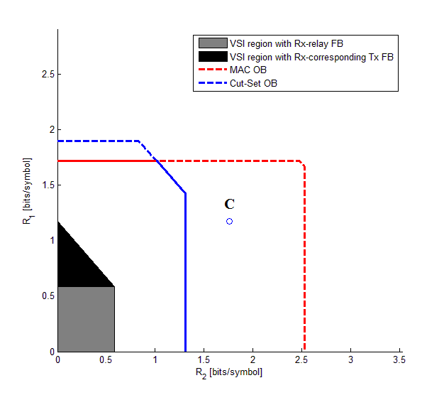
Figure 6: The capacity region of the ICRF in the VSI regime with Rx-relay feedback and without Rx-Tx feedback (the gray area) and the achievable region of Proposition 3 (gray and black area), when the channel is subject to phase fading and $P_{1}=P_{2}=P_{3}=10$, $a_{11}=0.2$, $a_{12}=0.44$, $a_{22}=0.2$, $a_{21}=0.27$ , $a_{13}=0.01$, $a_{23}=0.6$, $a_{31}=0.1$, and $a_{32}=0.1$. Point C corresponds to the rate pair $(R_{1},R_{2})=(I(X_{1},X_{2},X_{3};Y_{1}|\tilde{H}_{1}),I(X_{1},X_{2},X_{3};Y_{2}|\tilde{H}_{2}))$. Observe that this rate pair is outside the outer bound.

Comment 24.

Recall that in [51] it was shown that feedback can provide an unbounded gain as the SNR and INR increase to infinity. In [26] it was shown that an unbounded capacity gain can be obtained also for the weak interference regime. We note that these results deal with the degrees of freedom of the channel, thus the conclusion holds only when the SNR and INR increase to infinity. As to the present case, we show in Proposition 3 that the rate pair $(R_{1}^{*},R_{2}^{*})=(I(X_{1},X_{2},X_{3};Y_{1}|\tilde{H}_{1}),0)$ is achievable when $I(X_{1},X_{2},X_{3};Y_{1}|\tilde{H}_{1})\leq I(X_{1};Y_{2}|X_{2},X_{3},\tilde{H}_{2})$ holds. In the following we show that this implies an unbounded capacity gain over the no-feedback case for Rayleigh fading on the VSI regime.

Let $P_{1}=P_{2}=P_{3}=SNR$, Let $a_{11}$, $a_{13}$, $a_{22}$, $a_{23}$, $a_{31}$, $a_{32}$ be constants, and let $a_{12}=\alpha_{12}SNR^{\frac{b-1}{2}}$, $a_{21}=\alpha_{21}SNR^{\frac{a-1}{2}}$. Note that under these definitions

$$INR_{12} = a_{12}^{2}P_{1}=\alpha_{12}^{2}SNR^{b-1}SNR=\alpha_{12}SNR^{b}$$

$$INR_{21} = a_{21}P_{2}=\alpha_{21}SNR^{a}.$$

Now consider the condition $I(X_{1},X_{2},X_{3};Y_{1}|\tilde{H}_{1})\leq I(X_{1};Y_{2}|X_{2},X_{3},\tilde{H}_{2})$: Using the above definitions we obtain

$$\!\!\!\!\!\mathds{E}_{\tilde{U}_{1}}\Big{\{}\log_{2}\big{(}1+a_{11}^{2}|U_{11}|^{2}SNR$$

$$\quad+\alpha_{21}^{2}|U_{21}|^{2}SNR^{a}+a_{31}^{2}|U_{31}|^{2}SNR\big{)}\Big{\}}$$

$$\qquad\qquad\quad\leq\mathds{E}_{\tilde{U}_{2}}\left\{\log_{2}\left(1+\alpha_{12}^{2}|U_{12}|^{2}SNR^{b}\right)\right\}.$$

Taking $SNR\rightarrow\infty$ and restricting $a>1$ and $b>1$ we arrive to the equivalent relationship

$$\mathds{E}_{\tilde{U}_{1}}\Big{\{}\log_{2}\big{(}\alpha_{21}^{2}|U_{21}|^{2}SNR^{a}\big{)}\Big{\}}$$

$$\qquad\leq\mathds{E}_{\tilde{U}_{2}}\left\{\log_{2}\big{(}\alpha_{12}^{2}|U_{12}|^{2}SNR^{b}\big{)}\right\},$$

which requires $b\geq a$. When this holds, the asymptotic sum-rate (we consider only the maximal $R_{1}$ when $R_{2}=0$) is given by

$$\!\!\!\!\!\!\!\!\!\!\!\!\!\!\!\!\!\!\!\!\!\!\!\!\!\!\!\!\mathcal{C}_{\mbox{\scriptsize sum}}^{\mbox{\scriptsize FB-Tx+relay}}(R_{2}=0,SNR,a,b)$$

$$= I(X_{1},X_{2},X_{3};Y_{1}|\tilde{H}_{1})$$

$$= \mathds{E}_{\tilde{U}_{1}}\Big{\{}\log_{2}\big{(}1+a_{11}^{2}|U_{11}|^{2}SNR$$

$$\quad+\alpha_{21}^{2}|U_{21}|^{2}SNR^{a}+a_{31}^{2}|U_{31}|^{2}SNR\big{)}\Big{\}}$$

$$\stackrel{{\scriptstyle SNR\rightarrow\infty}}{{\longrightarrow}} \mathds{E}_{\tilde{U}_{1}}\Big{\{}\log_{2}\big{(}\alpha_{21}^{2}|U_{21}|^{2}SNR^{a}\big{)}\Big{\}}+O(1)$$

$$= a\log_{2}SNR+O(1),$$

where $O(1)$ means that for some $SNR$ large enough, the term is bounded by a constant, see, e.g. [58]. Next, we consider the sum-rate with feedback only to the relay, starting with the VSI regime. Recall that the same sum-rate is achieved without feedback when relay reception is good in the sense that the channel coefficients satisfy [17, Eqns. (8)]. Consider first the VSI condition (3b): $I(X_{2},X_{3};Y_{2}|X_{1},\tilde{H}_{2})\leq I(X_{2};Y_{1}|\tilde{H}_{1})$. Writing this explicitly we obtain

$$\!\!\!\!\mathds{E}_{\tilde{U}_{1}}\!\!\left\{\log_{2}\left(\!\!1+\frac{\alpha_{21}^{2}|U_{21}|^{2}SNR^{a}}{1+a_{11}^{2}|U_{11}|^{2}SNR+a_{31}^{2}|U_{31}|^{2}SNR}\right)\!\!\right\}$$

$$\geq\mathds{E}_{\tilde{U}_{2}}\!\Big{\{}\!\!\log_{2}\big{(}1+a_{22}^{2}|U_{22}|^{2}SNR+a_{32}^{2}|U_{32}|^{2}SNR\big{)}\Big{\}},$$

which, as $SNR\rightarrow\infty$, becomes

$$\!\!\!\!\mathds{E}_{\tilde{U}_{2}}\Big{\{}\log_{2}\big{(}(a_{22}^{2}|U_{22}|^{2}+a_{32}^{2}|U_{32}|^{2})SNR\big{)}\Big{\}}$$

$$\quad\leq\mathds{E}_{\tilde{U}_{1}}\left\{\log_{2}\left(\alpha_{21}^{2}|U_{21}|^{2}SNR^{a}\right)\right\}$$

$$\qquad\quad-\mathds{E}_{\tilde{U}_{1}}\left\{\log_{2}\left((a_{11}^{2}|U_{11}|^{2}+a_{31}^{2}|U_{31}|^{2})SNR\right)\right\}.$$

This inequality holds asymptotically when $a>2$. Similarly we can show that $I(X_{1},X_{3};Y_{1}|X_{2},\tilde{H}_{1})\leq I(X_{1};Y_{2}|\tilde{H}_{2})$ holds for $SNR\rightarrow\infty$ when $b>2$.

Recall that at asymptotically high SNR and INR, the VSI regime is defined as $a\geq 2$ and $b\geq 2$ (see [51], [26]. We thus conclude that with feedback only at the relay, the maximal achievable sum-rate at asymptotically high SNR in the VSI regime is

$$\!\!\!\mathcal{C}_{\mbox{\scriptsize sum}}^{\mbox{\scriptsize FB}}(SNR,a,b)$$

$$=I(X_{1},X_{3};Y_{1}|X_{2},\tilde{H}_{1})+I(X_{2},X_{3};Y_{2}|X_{1},\tilde{H}_{2})$$

$$=\mathds{E}_{\tilde{U}_{1}}\Big{\{}\log_{2}\big{(}1+a_{11}^{2}|U_{11}|^{2}SNR+a_{31}^{2}|U_{31}|^{2}SNR\big{)}\Big{\}}$$

$$\quad+\mathds{E}_{\tilde{U}_{2}}\!\Big{\{}\!\log_{2}\big{(}\!1+a_{22}^{2}|U_{22}|^{2}SNR+a_{32}^{2}|U_{32}|^{2}SNR\big{)}\!\Big{\}}$$

$$\stackrel{{\scriptstyle SNR\rightarrow\infty}}{{\longrightarrow}}\mathds{E}_{\tilde{U}_{1}}\Big{\{}\log_{2}\big{(}(a_{11}^{2}|U_{11}|^{2}+a_{31}^{2}|U_{31}|^{2})SNR\big{)}\Big{\}}$$

$$\quad\;\;\qquad+\mathds{E}_{\tilde{U}_{2}}\Big{\{}\log_{2}\big{(}(a_{22}^{2}|U_{22}|^{2}+a_{32}^{2}|U_{32}|^{2})SNR\big{)}\Big{\}}$$

$$=2\log_{2}SNR+O(1).$$

Comparing the sum-capacity with and without feedback to the transmitters we observe that in VSI

$$\frac{\mathcal{C}_{\mbox{\scriptsize sum}}^{\mbox{\scriptsize FB-Tx+relay}}(R_{2}=0,SNR,a,b)}{\mathcal{C}_{\mbox{\scriptsize sum}}^{\mbox{\scriptsize FB}}(SNR,a,b)}=\frac{a}{2}.$$

We conclude that adding feedback links from each receiver to the its corresponding transmitter allows an unbounded rate gain in the VSI regime. This follows directly from our capacity results.

VII ICRs with Partial Feedback at the Relay

In this section we study the scenarios in which only partial feedback is available at the relay. We consider the case where feedback is available only from Rx₁, the case where feedback is available only from Rx₂ is symmetric. This scenario is described in Fig. 7.

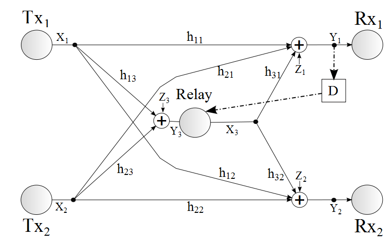
Figure 7: The interference channel with a relay and feedback only from Rx₁ to the relay. The ‘D’ block represents a single-symbol delay.

VII-A Partial Feedback in the Very Strong Interference Regime

First, we characterize the capacity region of the ICRF in the VSI regime for the case where the relay receives feedback only from Rx₁, i.e, $y_{1,1}^{i-1}$ and $\tilde{h}_{1,1}^{i-1}$ are available at the relay at time $i$ prior to transmission. In this scenario, the CSI at the relay is represented by $\underline{\tilde{H}}=\big{(}H_{13},H_{23},\tilde{H}_{1}\big{)}\in\mathfrak{C}^{5}\triangleq\underline{\tilde{\mathfrak{H}}}$. Thus, the encoder at the relay in (2) in Definition 1 is replaced by

$$x_{3,i}=t_{i}\big{(}y_{1,1}^{i-1},y_{3,1}^{i-1},h_{13,1}^{i-1},h_{23,1}^{i-1},\tilde{h}_{1,1}^{i-1}\big{)}\in\mathfrak{C},$$ (39)

$i=1,2,...,n$. The other definitions remain unchanged, as described in section II. Next, we have the following theorem:

Theorem 3.

Consider the fading ICRF with Rx-CSI. Assume that the channel coefficients are independent in time and independent of each other s.t. their phases are i.i.d. and distributed uniformly over $[0,2\pi)$. Let the additive noises be i.i.d. circularly symmetric complex Normal processes, $\mathcal{CN}(0,1)$, and let the sources have power constraints $\mathds{E}\big{\{}|X_{k}|^{2}\big{\}}\leq P_{k}$, $k\in\{1,2,3\}$. Assume that there is only one noiseless feedback link – from Rx₁ to the relay (see Fig. 7). If

$$I(X_{1},X_{3};Y_{1}|X_{2},\tilde{H}_{1}) \leq \min\big{\{}I(X_{1};Y_{1},Y_{3}|X_{2},X_{3},\underline{\tilde{H}}),$$ (40a)

$$\qquad\quad I(X_{1};Y_{2}|\tilde{H}_{2})\big{\}}$$

$$I(X_{2},X_{3};Y_{2}|X_{1},\tilde{H}_{2}) \leq I(X_{2};Y_{1}|\tilde{H}_{1}),$$ (40b)

where the mutual information expressions are evaluated with $X_{k}\sim\mathcal{CN}(0,P_{k}),k\in\{1,2,3\}$, mutually independent, then the capacity region is given by all the nonnegative rate pairs s.t.

$$R_{1}\leq I(X_{1},X_{3};Y_{1}|X_{2},\tilde{H}_{1})$$ (41a)

$$R_{2}\leq I(X_{2},X_{3};Y_{2}|X_{1},\tilde{H}_{2}),$$ (41b)

and it is achieved with $X_{k}\sim\mathcal{CN}(0,P_{k}),k\in\{1,2,3\}$, mutually independent and with DF strategy at the relay.

VII-A1 Proof of Theorem 3

The proof consists of the following steps:

• We obtain an outer bound on the capacity region using the cut-set bound.

• We show that the input distribution that maximizes the outer bound is zero-mean, circularly symmetric complex Normal with channel inputs independent of each other and with maximum allowed power.

• We derive an achievable rate region based on DF with partial feedback at the relay, using codebooks generated according to mutually independent, zero-mean circularly symmetric complex Normal input distributions.

  • We derive an achievable rate region for decoding at the relay using steps similar to [7, Sec. 4.D].

  • We obtain an achievable rate region for decoding at the destinations by decoding the interference first, while treating the relay signal and the desired signal as additive i.i.d. noises, followed by using a backward decoding scheme for decoding the desired message.

• We derive the VSI conditions which guarantee that decoding the interference first at each receiver, does not constrain the rate of the other pair.

• We obtain conditions on the channel coefficients that guarantee that the achievable rate region coincides with the cut-set bound and thus it is the capacity region of the ICR with partial feedback in the VSI regime.

We follow steps similar to the case in which full feedback is available at the relay, so we only provide a sketch of the proof.

An Outer Bound

An outer bound on the capacity region is given by the cut-set bound in (5). Following similar steps as in section IV-A1 and Appendix A, we conclude that the outer bound is maximized by mutually independent, zero-mean, circularly symmetric complex Normal channel inputs with maximum allowed power.

An Achievable Rate Region

The code construction and encoding process are similar to sections IV-A2 and IV-A2. Hence, following similar steps as in [7, Sec. 4.D], we conclude that an achievable rate region for decoding at the relay is given by

$$\!\!\!\!\!\!\!\!\!\!\!\!\!\!\!\!\!\!\!\!\mathcal{R}_{\mbox{\scriptsize{Relay Decoding}}}$$

$$\!\!\!\!\!\!\!\!\!\!\!\!=\bigg{\{}(R_{1},R_{2})\in\mathfrak{R}^{2}_{+}:$$

$$R_{1}\leq I(X_{1};Y_{1},Y_{3}|X_{2},X_{3},\underline{\tilde{H}})$$ (42a)

$$R_{2}\leq I(X_{2};Y_{1},Y_{3}|X_{1},X_{3},\underline{\tilde{H}})$$ (42b)

$$R_{1}+R_{2}\leq I(X_{1},X_{2};Y_{1},Y_{3}|X_{3},\underline{\tilde{H}})\bigg{\}}.$$ (42c)

At the destinations, Rx₁ can decode the interference if

$$R_{2}\leq I(X_{2};Y_{1}|\tilde{H}_{1}),$$ (43a)

and Rx₂ can decode the interference if

$$R_{1}\leq I(X_{1};Y_{2}|\tilde{H}_{2}).$$ (43b)

Thus, decoding the interference first, we obtain an achievable rate region for decoding at the destinations:

$$\!\!\!\!\!\!\!\!\!\!\!\!\!\!\!\!\!\mathcal{R}^{\prime}_{\mbox{\scriptsize{Destination Decoding}}}$$

$$\!\!\!\!\!\!\!\!\!\!\!\!\!\!\!=\bigg{\{}(R_{1},R_{2})\in\mathfrak{R}^{2}_{+}:$$

$$\!\!\!\!\!\!\!\!\!\!\!\!\!\!\!\!R_{1}\!\leq\!\min\big{\{}I(X_{1},X_{3};Y_{1}|X_{2},\tilde{H}_{1}),I(X_{1};Y_{2}|\tilde{H}_{2})\big{\}}$$ (44a)

$$\!\!\!\!\!\!\!\!\!\!\!\!\!\!\!\!R_{2}\!\leq\!\min\big{\{}I(X_{2},X_{3};Y_{2}|X_{1},\tilde{H}_{2}),I(X_{2};Y_{1}|\tilde{H}_{1})\big{\}}\!\!\bigg{\}}.$$ (44b)

Hence, an achievable rate region for the ICR with partial feedback is given by

$$\mathcal{R}_{\mbox{\scriptsize{Achievable}}}=\mathcal{R}_{\mbox{\scriptsize{Relay Decoding}}}\cap\mathcal{R}^{\prime}_{\mbox{\scriptsize{Destination Decoding}}}.$$ (45)

The Capacity Region

Next, we should guarantee that decoding the interference does not constrain the rates at the destinations, this is satisfied if

$$\!\!\!\!\!\!\!\!\!\!\!\!\!\!\!\!\!\!\!\!\!\!\!\!\!\!\!\!\!\!\!\!\!\min\big{\{}I(X_{1};Y_{1},Y_{3}|X_{2},X_{3},\underline{\tilde{H}}),I(X_{1},X_{3};Y_{1}|X_{2},\tilde{H}_{1})\big{\}}$$

$$\leq I(X_{1};Y_{2}|\tilde{H}_{2})$$

$$\!\!\!\!\!\!\!\!\!\!\!\!\!\!\!\!\!\!\!\!\!\!\!\!\!\!\!\!\!\!\!\!\!\min\big{\{}I(X_{2};Y_{1},Y_{3}|X_{1},X_{3},\underline{\tilde{H}}),I(X_{2},X_{3};Y_{2}|X_{1},\tilde{H}_{2})\big{\}}$$

$$\leq I(X_{2};Y_{1}|\tilde{H}_{1}).$$ (46b)

Note that as the channel inputs are mutually independent, we obtain that $I(X_{2};Y_{1}|\tilde{H}_{1})\leq I(X_{2};Y_{1},Y_{3}|X_{1},X_{3},\underline{\tilde{H}})$. Hence, the conditions in (46) can be reduced to

$$\!\!\!\!\!\!\!\!\!\!\!\!\!\!\!\!\!\!\!\!\!\!\!\!\!\!\!\!\!\!\!\!\!\!\!\!\!\!\!\!\!\!\!\!\!\!\!\!\!\!\!\!\!\!\!\!\!\!\!\!\!\!\!\!\min\big{\{}I(X_{1};Y_{1},Y_{3}|X_{2},X_{3},\underline{\tilde{H}}),I(X_{1},X_{3};Y_{1}|X_{2},\tilde{H}_{1})\big{\}}$$ (47a)

$$\leq I(X_{1};Y_{2}|\tilde{H}_{2})$$

$$I(X_{2},X_{3};Y_{2}|X_{1},\tilde{H}_{2}) \leq I(X_{2};Y_{1}|\tilde{H}_{1}).$$ (47b)

Finally, in order to achieve capacity, we should guarantee that, whenever the destinations can reliably decode their messages, the relay can decode both messages reliably. This can be done if

$$\!\!\!I(X_{1},X_{3};Y_{1}|X_{2},\tilde{H}_{1})\leq I(X_{1};Y_{1},Y_{3}|X_{2},X_{3},\underline{\tilde{H}})\phantom{xx}$$ (48a)

$$\!\!\!I(X_{2},X_{3};Y_{2}|X_{1},\tilde{H}_{2})\leq I(X_{2};Y_{1},Y_{3}|X_{1},X_{3},\underline{\tilde{H}})\phantom{xx}$$ (48b)

$$\!\!\!I(X_{1},X_{3};Y_{1}|X_{2},\tilde{H}_{1})$$

$$\!\!\!+I(X_{2},X_{3};Y_{2}|X_{1},\tilde{H}_{2})\leq I(X_{1},X_{2};Y_{1},Y_{3}|X_{3},\underline{\tilde{H}})\phantom{xx}.$$ (48c)

Recall that the channel inputs are independent, hence when (47b) holds, (48b) is always satisfied since

$$I(X_{2},X_{3};Y_{2}|X_{1},\tilde{H}_{2}) \leq I(X_{2};Y_{1}|\tilde{H}_{1})$$

$$\leq I(X_{2};Y_{1},Y_{3}|X_{3},\underline{\tilde{H}})$$

$$\leq I(X_{2};Y_{1},Y_{3}|X_{1},X_{3},\underline{\tilde{H}}).$$

Similar arguments show that when (47b) and (48a) hold, (48) is always satisfied:

$$\!\!\!\!\!\!I(X_{1},X_{2};Y_{1},Y_{3}|X_{3},\underline{\tilde{H}})$$

$$=I(X_{2};Y_{1},Y_{3}|X_{3},\underline{\tilde{H}})+I(X_{1};Y_{1},Y_{3}|X_{2},X_{3},\underline{\tilde{H}})$$

$$\geq I(X_{2},X_{3};Y_{2}|X_{1},\tilde{H}_{2})+I(X_{1},X_{3};Y_{1}|X_{2},\tilde{H}_{1}).$$

Therefore, if (47b) holds, (48a) is enough to guarantee reliable decoding at the relay (i.e., (42) is satisfied).

Finally note that by combining (47) with (48a) we obtain conditions which coincide with (40) and under these conditions (45) specialize to (41). Comparing with the cut-set bound in (5), we conclude that if (40) holds, the achievable rate region (41), coincides with the cut-set bounds and hence it is the capacity region. $\blacksquare$

VII-A2 Ergodic Phase Fading

When the channel is subject to ergodic phase fading, we obtain the following explicit result:

Corollary 6.

Consider the phase fading ICR with Rx-CSI and partial feedback s.t. $y_{1,1}^{i-1}$ and $\tilde{h}_{1,1}^{i-1}$ are available at the relay at time $i$. If the channel coefficients satisfy

$$a_{11}^{2}P_{1}+a_{31}^{2}P_{3} \leq \min\Big{\{}\frac{a_{12}^{2}P_{1}}{1+a_{22}^{2}P_{2}+a_{32}^{2}P_{3}},$$ (49a)

$$\qquad\qquad(a_{11}^{2}+a_{13}^{2})P_{1}\Big{\}}$$

$$a_{22}^{2}P_{2}+a_{32}^{2}P_{3} \leq \frac{a_{21}^{2}P_{2}}{1+a_{11}^{2}P_{1}+a_{31}^{2}P_{3}},$$ (49b)

then the capacity region is characterized by all the nonnegative rate pairs s.t.

$$R_{1} \leq \log_{2}\big{(}1+a_{11}^{2}P_{1}+a_{31}^{2}P_{3}\big{)}$$ (50a)

$$R_{2} \leq \log_{2}\big{(}1+a_{22}^{2}P_{2}+a_{32}^{2}P_{3}\big{)},$$ (50b)

and it is achieved with $X_{k}\sim\mathcal{CN}(0,P_{k}),k\in\{1,2,3\}$, mutually independent and with DF strategy at the relay.

Proof.

The result follows from the expressions of Theorem 3. In order to obtain the conditions on the channel coefficients in (49), we evaluate $I(X_{1};Y_{1},Y_{3}|X_{2},X_{3},\underline{\tilde{H}})$ using mutually independent, zero-mean circularly symmetric complex Normal channel inputs. This leads to

$$\!\!\!\!\!\!\!\!I(X_{1};Y_{1},Y_{3}|X_{2},X_{3},\underline{\tilde{H}})$$

$$\quad=\mathds{E}_{\underline{\tilde{H}}}\bigg{\{}\log_{2}\Big{(}1+P_{1}(|H_{11}|^{2}+|H_{13}|^{2})\Big{)}\bigg{\}}.$$ (51)

Next, note that under the phase fading model $|H_{11}|^{2}=a_{11}^{2}$ and $|H_{13}|^{2}=a_{13}^{2}$, thus (VII-A2) can be rewritten as

$$I(X_{1};Y_{1},Y_{3}|X_{2},X_{3},\underline{\tilde{H}})=\log_{2}\big{(}1+P_{1}(a_{11}^{2}+a_{13}^{2})\big{)}.$$

The rest of the expressions in Theorem 3 have been already evaluated for the phase fading model in Corollary 1. ∎

VII-A3 Ergodic Rayleigh Fading

Define $\tilde{U}_{k}\triangleq(U_{kk},U_{3k}),\hat{U}_{k}\triangleq(U_{1k},U_{2k},U_{3k}),k\in\{1,2\}$. If the channel is subject to ergodic Rayleigh fading, we obtain the following explicit result:

Corollary 7.

Consider the Rayleigh fading ICR with Rx-CSI and partial feedback s.t. $y_{1,1}^{i-1}$ and $\tilde{h}_{1,1}^{i-1}$ are available at the relay at time $i$. If the channel coefficients satisfy

$$\!\!\!\!\!\!\!\!\!\!\!\!\!\!\mathds{E}_{\tilde{U}_{1}}\Big{\{}\!\log_{2}\big{(}1\!+\!a_{11}^{2}|U_{11}|^{2}P_{1}\!+\!a_{31}^{2}|U_{31}|^{2}P_{3}\big{)}\Big{\}}$$

$$\!\!\!\!\!\!\!\!\!\!\!\!\!\leq\mathds{E}_{U_{11},U_{13}}\Big{\{}\!\log_{2}\big{(}1\!+\!(a_{11}^{2}|U_{11}|^{2}\!+\!a_{13}^{2}|U_{13}|^{2})P_{1}\big{)}\!\Big{\}}$$ (52a)

$$\!\!\!\!\!\!\!\!\!\!\!\!\!\!\mathds{E}_{\tilde{U}_{1}}\Big{\{}\log_{2}\big{(}1+a_{11}^{2}|U_{11}|^{2}P_{1}+a_{31}^{2}|U_{31}|^{2}P_{3}\big{)}\Big{\}}$$

$$\!\!\!\!\!\!\!\!\!\!\!\!\!\leq\mathds{E}_{\hat{U}_{2}}\!\!\left\{\!\log_{2}\!\left(\!1\!+\!\frac{a_{12}^{2}|U_{12}|^{2}P_{1}}{1\!+\!a_{22}^{2}|U_{22}|^{2}P_{2}\!+\!a_{32}^{2}|U_{32}|^{2}P_{3}}\right)\!\right\}$$ (52b)

$$\!\!\!\!\!\!\!\!\!\!\!\!\!\!\mathds{E}_{\tilde{U}_{2}}\!\Big{\{}\!\log_{2}\big{(}1\!+\!a_{22}^{2}|U_{22}|^{2}P_{2}\!+\!a_{32}^{2}|U_{32}|^{2}P_{3}\big{)}\!\Big{\}}$$

$$\!\!\!\!\!\!\!\!\!\!\!\!\!\leq\mathds{E}_{\hat{U}_{1}}\!\!\left\{\!\log_{2}\!\left(\!1\!+\!\frac{a_{21}^{2}|U_{21}|^{2}P_{2}}{1\!+\!a_{11}^{2}|U_{11}|^{2}P_{1}\!+\!a_{31}^{2}|U_{31}|^{2}P_{3}}\right)\!\right\}$$ (52c)

then the capacity region is characterized by all the nonnegative rate pairs s.t.

$$\!\!\!\!\!\!\!\!\!\!\!\!\!\!\!\!\!R_{1}\leq\mathds{E}_{\tilde{U}_{1}}\Big{\{}\!\log_{2}\big{(}1\!+\!a_{11}^{2}|U_{11}|^{2}P_{1}\!+\!a_{31}^{2}|U_{31}|^{2}P_{3}\big{)}\!\Big{\}}$$ (53a)

$$\!\!\!\!\!\!\!\!\!\!\!\!\!\!\!\!\!R_{2}\leq\mathds{E}_{\tilde{U}_{2}}\Big{\{}\!\log_{2}\big{(}1\!+\!a_{22}^{2}|U_{22}|^{2}P_{2}\!+\!a_{32}^{2}|U_{32}|^{2}P_{3}\big{)}\!\Big{\}},$$ (53b)

and it is achieved with $X_{k}\sim\mathcal{CN}(0,P_{k}),k\in\{1,2,3\}$, mutually independent and with DF strategy at the relay.

Proof.

The proof follows similar arguments to those used in the proof of Corollary 6. ∎

VII-A4 Comments

Comment 25.

Comparing to Theorem 1, we observe that in Theorem 3 there is an additional condition in (40). This is due to the fact that with partial feedback at the relay, the cut-set bound cannot be achieved at the destination without guaranteeing reliable decoding at the relay.

Comment 26.

For the configuration described in Theorem 3, then from Proposition 2 it is clear that adding a noiseless feedback link, from Rx₁ to Tx₂ (partial Rx-opposite Tx feedback) does not enlarge the capacity region in the VSI regime.

Comment 27.

Consider the configuration described in Theorem 3 with an additional noiseless feedback link from Rx₁ to Tx₁ (partial Rx-corresponding Tx feedback). Then, following the same arguments as in Proposition 3, we conclude that if

$$\!\!\!\!\!\!\!\!\!\!I(X_{1},X_{3};Y_{1}|X_{2},\tilde{H}_{1}) \!\leq\! \min\big{\{}I(X_{1};Y_{2}|\tilde{H}_{2}),$$ (54a)

$$I(X_{1};Y_{1},Y_{3}|X_{2},X_{3},\underline{\tilde{H}})\!\big{\}}$$

$$\!\!\!\!\!\!\!\!\!\!I(X_{1},X_{2},X_{3};Y_{2}|\tilde{H}_{2}) \!\leq\! I(X_{2};Y_{1}|\tilde{H}_{1}),$$ (54b)

hold, then $(R_{1},R_{2})=\big{(}0,I(X_{1},X_{2},X_{3};Y_{2}|\tilde{H}_{2})\big{)}$ is achievable. Note that (54) guarantees (40). Hence, when partial feedback (only from Rx₁) is available at the relay, then an additional feedback link from Rx₁ to Tx₁ increases the capacity region in the VSI regime. Figure 8 demonstrates the corresponding capacity region.

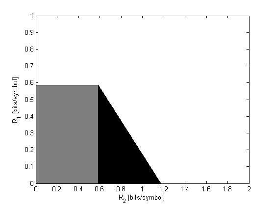
Figure 8: The capacity region of the ICRF in the VSI regime with Rx₁-relay feedback and without Rx-Tx feedback (the gray area) and the achievable region with Rx₁-relay and Rx₁-Tx₁ feedback (gray and black area), when the channel is subject to phase fading and $P_{1}=P_{2}=P_{3}=10,a_{11}=0.2,a_{12}=0.27,a_{21}=0.44,a_{22}=0.2,a_{31}=0.1,a_{32}=0.1$ and $a_{13}=0.3$.

VII-B Partial Feedback in the Strong Interference Regime

In this section, we characterize the capacity region of the ICR with partial feedback in the strong interference regime. We consider the case in which feedback is available only from Rx₁.

Theorem 4.

For the scenario of Theorem 3, if the channel coefficients satisfy

$$\!\!\!\!\!\!\!\!\!\!\!I(X_{1},X_{3};Y_{2}|X_{2},\tilde{H}_{2}) \!\leq\! I(X_{1};Y_{1},Y_{3}|X_{2},X_{3},\underline{\tilde{H}})$$ (55a)

$$\!\!\!\!\!\!\!\!\!\!\!I(X_{2},X_{3};Y_{1}|X_{1},\tilde{H}_{1}) \!\leq\! I(X_{2};Y_{1},Y_{3}|X_{1},X_{3},\underline{\tilde{H}})$$ (55b)

$$\!\!\!\!\!\!\!\!\!\!\!I(X_{1},X_{2},X_{3};Y_{2}|\tilde{H}_{2}) \!\leq\! I(X_{1},X_{2};Y_{1},Y_{3}|X_{3},\underline{\tilde{H}})$$ (55c)

$$\!\!\!\!\!\!\!\!\!\!\!I(X_{1},X_{3};Y_{1}|X_{2},\tilde{H}_{1}) \!\leq\! I(X_{1};Y_{2}|X_{2},\tilde{H}_{2})$$ (55d)

$$\!\!\!\!\!\!\!\!\!\!\!I(X_{2},X_{3};Y_{2}|X_{1},\tilde{H}_{2}) \!\leq\! I(X_{2};Y_{1}|X_{1},\tilde{H}_{1}),$$ (55e)

where the mutual information expressions are evaluated with $X_{k}\sim\mathcal{CN}(0,P_{k}),k\in\{1,2,3\}$, mutually independent, then the capacity region is given by all the nonnegative rate pairs s.t.

$$\!\!\!\!R_{1} \leq I(X_{1},X_{3};Y_{1}|X_{2},\tilde{H}_{1})$$ (56a)

$$\!\!\!\!R_{2} \leq I(X_{2},X_{3};Y_{2}|X_{1},\tilde{H}_{2})$$ (56b)

$$\!\!\!\!R_{1}+R_{2} \leq \min\big{\{}I(X_{1},X_{2},X_{3};Y_{1}|\tilde{H}_{1}),$$ (56c)

$$\quad\quad\qquad I(X_{1},X_{2},X_{3};Y_{2}|\tilde{H}_{2})\big{\}},$$

and it is achieved with $X_{k}\sim\mathcal{CN}(0,P_{k}),k\in\{1,2,3\}$, mutually independent and with DF strategy at the relay.

VII-B1 Proof of Theorem 4

The proof consists of the following steps:

• From the ICRF we obtain two component channels: the first is the MARC with feedback (MARCF) which is a MARC whose message destination is Rx₁ and the relay receives feedback only from Rx₁. The MARCF is defined by equations (1a) and (1c). The second is the partially enhanced MARC (PEMARC) defined as a MARC whose message destination is Rx₂, while the relay receives feedback from Rx₁. The PEMARC is defined by equations (1) and $(y_{1,1}^{i-1},\tilde{h}_{1,1}^{i-1})$ denotes the available feedback at the relay at time $i$ in both components. Note that contrary to Theorem 2, in the present case the component channels are not symmetric.

• We obtain the conditions on the channel coefficients s.t. the capacity of the MARCF and the PEMARC is achieved with DF at the relay. We show that for each component, capacity is achieved with zero-mean, circularly symmetric complex Normal channel inputs.

• We show that the same coding strategy at the sources and at the relay achieves capacity for both the MARCF and the PEMARC simultaneously.

• We therefore provide an achievable rate region for the ICR with partial feedback as the intersection of the capacity regions of the MARCF and the PEMARC.

• We show that when the conditions for SI are satisfied, the intersection of the capacity regions of the MARCF and the PEMARC contains the capacity region of the ICR with partial feedback.

• We conclude the capacity region of the ICR with partial feedback in the SI regime, to be the intersection of the capacity regions of the MARCF and the PEMARC.

• We explicitly characterize the SI conditions for the ICR with partial feedback.

An Achievable Rate Region

Recall the achievable rate region for decoding at the destination as in Theorem 2. Define $\underline{\mathbf{a}}$ as in section V-A1 and let $\mathcal{C}_{\scriptsize{\mbox{MARCF}}}(\underline{\mathbf{a}})$ and $\mathcal{C}_{\scriptsize{\mbox{PEMARC}}}(\underline{\mathbf{a}})$ denote the capacity regions of the MARCF and the PEMARC, respectively. Moreover, let $t_{1}(R_{1},R_{2})$ and $t_{2}(R_{1},R_{2})$ denote the coding strategy for the MARCF and the PEMARC, respectively. From the derivation in Appendix B it follows that when only partial feedback is available at the relay, achievable rate regions for the MARCF and the PEMARC obtained with DF at the relay are given by

$$\!\!\!\!\!\!\!\!\!\!\mathcal{R}^{\prime}_{\scriptsize{\mbox{MARCF/PEMARC}}}$$

$$\!\!\!\!=\bigg{\{}(R_{1},R_{2})\in\mathfrak{R}^{2}_{+}:$$

$$\qquad R_{1}\leq\min\big{\{}I(X_{1};Y_{1},Y_{3}|X_{2},X_{3},\underline{\tilde{H}}),$$

$$\qquad\qquad\qquad I(X_{1},X_{3};Y_{m}|X_{2},\tilde{H}_{m})\big{\}}$$ (57a)

$$\qquad R_{2}\leq\min\big{\{}I(X_{2};Y_{1},Y_{3}|X_{2},X_{3},\underline{\tilde{H}}),$$

$$\qquad\qquad\qquad I(X_{2},X_{3};Y_{m}|X_{1},\tilde{H}_{m})\big{\}}$$ (57b)

$$\qquad R_{1}+R_{2}\leq\min\big{\{}I(X_{1},X_{2};Y_{1},Y_{3}|X_{3},\underline{\tilde{H}}),$$

$$\qquad\qquad\qquad I(X_{1},X_{2},X_{3};Y_{m}|\tilde{H}_{m})\big{\}}\bigg{\}},$$ (57c)

where $m=1$ for the MARCF and $m=2$ for the PEMARC, and decoding at the relay at block $b$ is done using rule (IV-A2) without considering $\mathbf{y}_{2}(b)$, and $X_{k}\sim\mathcal{CN}(0,P_{k}),k\in\{1,2,3\}$, mutually independent. Let $t_{DF}(R_{1},R_{2})$ denote the coding scheme with mutually independent complex Normal inputs, achieving rates $R_{1}$ and $R_{2}$ in each component channel. Following steps similar to Appendix A, we can show that in order for $t_{DF}(R_{1},R_{2})$ to achieve the capacity of each component channel, we should guarantee that the relay decodes both messages reliably, i.e., we should guarantee that

$$\!\!\!\!\!\!\!\!\!\!\!\!\!\!\!\!\max_{k\in\{1,2\}}\left\{I(X_{1},X_{3};Y_{k}|X_{2},\tilde{H}_{k})\right\}$$

$$\qquad\qquad\leq I(X_{1};Y_{1},Y_{3}|X_{2},X_{3},\underline{\tilde{H}})$$ (58a)

$$\!\!\!\!\!\!\!\!\!\!\!\!\!\!\!\!\max_{k\in\{1,2\}}\left\{I(X_{2},X_{3};Y_{k}|X_{1},\tilde{H}_{k})\right\}$$

$$\qquad\qquad\leq I(X_{2};Y_{1},Y_{3}|X_{1},X_{3},\underline{\tilde{H}})$$ (58b)

$$\!\!\!\!\!\!\!\!\!\!\!\!\!\!\!\!\max_{k\in\{1,2\}}\left\{I(X_{1},X_{2},X_{3};Y_{k}|\tilde{H}_{k})\right\}$$

$$\qquad\qquad\leq I(X_{1},X_{2};Y_{1},Y_{3}|X_{3},\underline{\tilde{H}}).$$ (58c)

Note that if (58) holds then the capacity regions of the component channels are given by:

$$\!\!\!\!\!\!\!\!\!\!\!\!\!\!\!\!\mathcal{C}_{\scriptsize{\mbox{MARCF/PEMARC}}}(\underline{\mathbf{a}})$$

$$\!\!\!\!\!\!\!\!=\bigg{\{}(R_{1},R_{2})\in\mathfrak{R}^{2}_{+}:$$

$$\quad\quad R_{1}\leq I(X_{1},X_{3};Y_{m}|X_{2},\tilde{H}_{m})$$ (59a)

$$\quad\quad R_{2}\leq I(X_{2},X_{3};Y_{m}|X_{1},\tilde{H}_{m})$$ (59b)

$$\quad\quad R_{1}+R_{2}\leq I(X_{1},X_{2},X_{3};Y_{m}|\tilde{H}_{m})\bigg{\}},$$ (59c)

where $m=1$ for the MARCF and $m=2$ for the PEMARC, and they are achieved with $X_{k}\sim\mathcal{CN}(0,P_{k}),k\in\{1,2,3\}$, mutually independent and with DF strategy at the relay.

Note that when the conditions in (58) hold, by following similar steps as in the proof of Proposition 1 we conclude that the same coding strategy achieves capacity for both component channels simultaneously. Let $\mathcal{R}_{\scriptsize{\mbox{MARCF}}}\big{(}\underline{\mathbf{a}},t_{1}(R_{1},R_{2})\big{)}$ and $\mathcal{R}_{\scriptsize{\mbox{PEMARC}}}\big{(}\underline{\mathbf{a}},t_{2}(R_{1},R_{2})\big{)}$ denote the achievable rate regions of the MARCF and the PEMARC, respectively. Hence, when (58) holds and by choosing $t_{1}=t_{2}=t_{DF}$, any achievable rate pair $(R_{1},R_{2})\in\mathcal{R}_{\scriptsize{\mbox{MARCF}}}\big{(}\underline{\mathbf{a}},t_{DF}(R_{1},R_{2})\big{)}\cap\mathcal{R}_{\scriptsize{\mbox{PEMARC}}}\big{(}\underline{\mathbf{a}},t_{DF}(R_{1},R_{2})\big{)}$ is also achievable in the ICR with partial feedback. Thus, if (58) holds then an achievable rate region for the ICR with partial feedback is given by

$$\mathcal{R}_{\scriptsize{ICRF}}(\underline{\mathbf{a}},t_{DF}) = \mathcal{R}_{\scriptsize{\mbox{MARCF}}}(\underline{\mathbf{a}},t_{DF})\cap\mathcal{R}_{\scriptsize{\mbox{PEMARC}}}(\underline{\mathbf{a}},t_{DF})$$ (60)

$$= \mathcal{C}_{\scriptsize{\mbox{MARCF}}}(\underline{\mathbf{a}})\cap\mathcal{C}_{\scriptsize{\mbox{PEMARC}}}(\underline{\mathbf{a}})$$

$$\subseteq \mathcal{C}_{\scriptsize{\mbox{ICRF}}}(\underline{\mathbf{a}}).$$

Converse

The proof of the converse follows similar arguments to those used in section V-A2. Note that in the SI regime, both receivers can decode both messages without reducing the capacity region. Thus, any achievable rate pair $(R_{1},R_{2})\in\mathcal{C}_{\scriptsize{\mbox{ICRF}}}(\underline{\mathbf{a}})$ is also achievable in the component channels, i.e., $\mathcal{C}_{\scriptsize{\mbox{ICRF}}}(\underline{\mathbf{a}})\subseteq\mathcal{C}_{\scriptsize{\mbox{MARCF}}}(\underline{\mathbf{a}})\cap\mathcal{C}_{\scriptsize{\mbox{PEMARC}}}(\underline{\mathbf{a}})$. Thus, combined with (60) we conclude that in the SI regime

$$\mathcal{C}_{\scriptsize{\mbox{ICRF}}}(\underline{\mathbf{a}})=\mathcal{C}_{\scriptsize{\mbox{MARCF}}}(\underline{\mathbf{a}})\cap\mathcal{C}_{\scriptsize{\mbox{PEMARC}}}(\underline{\mathbf{a}}).$$ (61)

Recall that when decoding at the relay does not constrain the rates, then $\mathcal{C}_{\scriptsize{\mbox{MARCF}}}(\underline{\mathbf{a}})$ and $\mathcal{C}_{\scriptsize{\mbox{PEMARC}}}(\underline{\mathbf{a}})$ are given in (59). Next, we determine the SI conditions in the ICR with partial feedback. Note that since $\mathcal{C}_{\scriptsize{\mbox{MARCF}}}(\underline{\mathbf{a}})$ and $\mathcal{C}_{\scriptsize{\mbox{PEMARC}}}(\underline{\mathbf{a}})$ in (59) are achieved with $t_{DF}(R_{1},R_{2})$, for the rest of the proof we only consider mutually independent, circularly symmetric complex Normal channel inputs with zero mean. Recall the converse proof in V-A2 and consider any rate pair $(R_{1},R_{2})\in\mathcal{C}_{\scriptsize{\mbox{ICRF}}}(\underline{\mathbf{a}})$. If Rx₁ can decode $m_{1}$ from the signal

$$\mathbf{y}_{1}=\mathbf{h}_{11}\cdot\mathbf{x}_{1}+\mathbf{h}_{21}\cdot\mathbf{x}_{2}+\mathbf{h}_{31}\cdot\mathbf{x}_{3}+\mathbf{z}_{1},$$

then it can create the signal

$$\mathbf{y}_{1}^{\prime}=\mathbf{h}_{21}\cdot\mathbf{x}_{2}+\mathbf{h}_{31}\cdot\mathbf{x}_{3}+\mathbf{z}_{1},$$

from which it can decode $m_{2}$ by treating $\mathbf{h}_{31}\cdot\mathbf{x}_{3}$ as additive i.i.d. noise if

$$R_{2}\leq I(X_{2};Y_{1}^{\prime}|\tilde{H}_{1})\triangleq R_{2}^{\prime},$$

and similarly Rx₂ can decode $m_{1}$ if

$$R_{1}\leq I(X_{1};Y_{2}^{\prime}|\tilde{H}_{2})\triangleq R_{1}^{\prime}.$$

In order to guarantee that decoding both messages at each receiver does not reduce the capacity region we should require: $\max R_{1}\leq R_{1}^{\prime}$ and $\max R_{2}\leq R_{2}^{\prime}$. This is satisfied if

$$\!\!\!\!\!\!\!\!\!\!\sup_{f(x_{1},x_{2},x_{3})}\Big{\{}I(X_{1},X_{3};Y_{1}|X_{2},\tilde{H}_{1})\Big{\}}\!\leq\!I(X_{1};Y_{2}^{\prime}|\tilde{H}_{2})$$

$$\qquad\qquad\qquad\qquad\!\stackrel{{\scriptstyle(a)}}{{=}}I(X_{1};Y_{2}|X_{2},\tilde{H}_{2})$$ (62a)

$$\!\!\!\!\!\!\!\!\!\!\sup_{f(x_{1},x_{2},x_{3})}\Big{\{}I(X_{2},X_{3};Y_{2}|X_{1},\tilde{H}_{2})\Big{\}}\!\leq\!I(X_{2};Y_{1}^{\prime}|\tilde{H}_{1})$$

$$\qquad\qquad\qquad\qquad\!=\!I(X_{2};Y_{1}|X_{1},\tilde{H}_{1}).$$ (62b)

Note that all the above mutual information expressions are evaluated using the same channel input distribution. Here, (a) follows from the fact that the l.h.s. of (62) is maximized by $X_{k}\sim\mathcal{CN}(0,P_{k}),k\in\{1,2,3\}$, mutually independent and independent of the channel coefficients. Thus, when (58) holds, the conditions for the strong interference are given by

$$I(X_{1},X_{3};Y_{1}|X_{2},\tilde{H}_{1}) \leq I(X_{1};Y_{2}|X_{2},\tilde{H}_{2})$$ (63a)

$$I(X_{2},X_{3};Y_{2}|X_{1},\tilde{H}_{2}) \leq I(X_{2};Y_{1}|X_{1},\tilde{H}_{1}).$$ (63b)

We conclude that if the conditions for reliable decoding at the relay (58) and the conditions for SI (63) are satisfied, then the capacity region is given in (61) where the rate expressions for the component channels are given in (59).

Simplification of the Capacity Region

Next, note that when (63) is satisfied, we obtain

$$I(X_{1},X_{3};Y_{1}|X_{2},\tilde{H}_{1}) \leq I(X_{1};Y_{2}|X_{2},\tilde{H}_{2})$$

$$\leq I(X_{1},X_{3};Y_{2}|X_{2},\tilde{H}_{2})$$

$$I(X_{2},X_{3};Y_{2}|X_{1},\tilde{H}_{2}) \leq I(X_{2};Y_{1}|X_{1},\tilde{H}_{1})$$

$$\leq I(X_{2},X_{3};Y_{1}|X_{1},\tilde{H}_{1}),$$

hence, (61) can be reduced to

$$R_{1} \leq I(X_{1},X_{3};Y_{1}|X_{2},\tilde{H}_{1})$$ (64a)

$$R_{2} \leq I(X_{2},X_{3};Y_{2}|X_{1},\tilde{H}_{2})$$ (64b)

$$R_{1}+R_{2} \leq \min\big{\{}I(X_{1},X_{2},X_{3};Y_{1}|\tilde{H}_{1}),$$ (64c)

$$\qquad\quad I(X_{1},X_{2},X_{3};Y_{2}|\tilde{H}_{2})\big{\}},$$

and (58) can be reduced to

$$\!\!\!\!\!\!\!\!\!\!I(X_{1},X_{3};Y_{2}|X_{2},\tilde{H}_{2})$$

$$\qquad\qquad\leq I(X_{1};Y_{1},Y_{3}|X_{2},X_{3},\underline{\tilde{H}})$$ (65a)

$$\!\!\!\!\!\!\!\!\!\!I(X_{2},X_{3};Y_{1}|X_{1},\tilde{H}_{1})$$

$$\qquad\qquad\leq I(X_{2};Y_{1},Y_{3}|X_{1},X_{3},\underline{\tilde{H}})$$ (65b)

$$\!\!\!\!\!\!\!\!\!\!\max_{k\in\{1,2\}}\left\{I(X_{1},X_{2},X_{3};Y_{k}|\tilde{H}_{k})\right\}$$

$$\qquad\qquad\leq I(X_{1},X_{2};Y_{1},Y_{3}|X_{3},\underline{\tilde{H}}).$$ (65c)

Next, note that when (63a) and (65) hold, we obtain

$$\!\!\!\!\!\!\!\!\!\!\!\!\!I(X_{1},X_{2},X_{3};Y_{1}|\tilde{H}_{1})$$

$$= I(X_{2};Y_{1}|\tilde{H}_{1})+I(X_{1},X_{3};Y_{1}|X_{2},\tilde{H}_{1})$$

$$\leq I(X_{2};Y_{1}|\tilde{H}_{1})+I(X_{1},X_{3};Y_{2}|X_{2},\tilde{H}_{2})$$

$$\leq I(X_{2};Y_{1},Y_{3}|X_{3},\underline{\tilde{H}})+I(X_{1};Y_{1},Y_{3}|X_{2},X_{3},\underline{\tilde{H}})$$

$$= I(X_{1},X_{2};Y_{1},Y_{3}|X_{3},\underline{\tilde{H}}).$$

Therefore, if (63) holds, (65) reduces to

$$\!\!\!\!\!\!\!\!I(X_{1},X_{2},X_{3};Y_{2}|\tilde{H}_{2}) \leq I(X_{1},X_{2};Y_{1},Y_{3}|X_{3},\underline{\tilde{H}}).$$ (66)

Observe that in the SI regime with partial feedback, reliable decoding at the relay does not constrain the sum-rate in the MARCF. In the PEMARC, however, (66) constrains the sum-rate to guarantee reliable decoding at the relay. Hence, decoding at the relay imposes an additional condition on the channel coefficients in the PEMARC onto those required in the MARCF. Note that (64) gives (56) and by combining (63) with (65), (65) and (66), we obtain the conditions in (55). This completes the proof. $\blacksquare$

VII-B2 Ergodic Phase Fading

Define $\tilde{\underline{\theta}}\triangleq(\theta_{11},\theta_{13},\theta_{21},\theta_{23})$. When the channel is subject to ergodic phase fading, we obtain the following explicit result:

Corollary 8.

Consider the phase fading ICR with Rx-CSI and partial feedback s.t. $y_{1,1}^{i-1}$ and $\tilde{h}_{1,1}^{i-1}$ are available at the relay at time $i$. If the channel coefficients satisfy

$$a_{12}^{2}P_{1}+a_{32}^{2}P_{3} \leq (a_{11}^{2}+a_{13}^{2})P_{1}$$ (67a)

$$a_{21}^{2}P_{2}+a_{31}^{2}P_{3} \leq (a_{21}^{2}+a_{23}^{2})P_{2}$$ (67b)

$$\!\!\!\!\!\!\!\!\!\!\!\!\log_{2}\big{(}1\!+\!a_{12}^{2}P_{1}\!+\!a_{22}^{2}P_{2}\!+\!a_{32}^{2}P_{3}\big{)} \leq$$ (67c)

$$\!\!\!\!\!\!\!\!\!\!\!\!\!\!\!\!\!\!\!\!\!\!\!\!\!\!\!\!\!\!\!\!\!\!\!\!\!\!\!\!\!\!\!\!\!\!\!\!\!\!\!\!\!\!\!\!\!\!\!\!\!\!\!\!\!\!\!\!\!\!\!\!\!\!\!\!\!\!\!\!\!\!\!\!\!\mathds{E}_{\tilde{\underline{\theta}}}\bigg{\{}\log_{2}\Big{(}1+\big{(}\sum_{k=1}^{2}P_{k}\cdot(a_{k1}^{2}+a_{k3}^{2})\big{)}$$

$$\!\!\!\!\!\!\!\!\!\!\!\!\!\!\!\!\!\!\!\!\!\!\!\!\!\!\!\!\!\!\!\!\!\!\!\!\!\!\!\!\!\!\!\!\!\!\!\!\!\!\!\!\!\!\!+P_{1}P_{2}\cdot\big{(}a_{11}^{2}a_{23}^{2}+a_{13}^{2}a_{21}^{2}$$

$$\!\!\!\!\!\!\!\!\!\!\!\!\!\!\!\!\!\!\!\!\!\!\!\!\!\!\!\!\!\!\!\!\!\!\!\!\!\!\!\!\!\!\!\!\!\!\!\!\!\!\!\!\!\!\!-2\cdot a_{13}a_{21}a_{11}a_{23}\cdot\cos(\theta_{13}+\theta_{21}$$

$$\!\!\!\!\!\!\!\!\!\!\!\!\!\!\!\!\!\!\!\!\!\!\!-\theta_{11}-\theta_{23})\big{)}\Big{)}\bigg{\}}$$

$$a_{11}^{2}P_{1}+a_{31}^{2}P_{3} \leq \frac{a_{12}^{2}P_{1}}{1+a_{32}^{2}P_{3}}$$ (67d)

$$a_{22}^{2}P_{2}+a_{32}^{2}P_{3} \leq \frac{a_{21}^{2}P_{2}}{1+a_{31}^{2}P_{3}},$$ (67e)

then the capacity region is characterized by all the nonnegative rate pairs s.t.

$$R_{1} \leq \log_{2}\big{(}1+a_{11}^{2}P_{1}+a_{31}^{2}P_{3}\big{)}$$ (68a)

$$R_{2} \leq \log_{2}\big{(}1+a_{22}^{2}P_{2}+a_{32}^{2}P_{3}\big{)}$$ (68b)

$$R_{1}+R_{2} \leq \min\Big{\{}\log_{2}\big{(}1+a_{11}^{2}P_{1}+a_{21}^{2}P_{2}+a_{31}^{2}P_{3}\big{)},$$ (68c)

$$\log_{2}\big{(}1+a_{12}^{2}P_{1}+a_{22}^{2}P_{2}+a_{32}^{2}P_{3}\big{)}\Big{\}},$$

and it is achieved with $X_{k}\sim\mathcal{CN}(0,P_{k}),k\in\{1,2,3\}$, mutually independent and with DF strategy at the relay.

Proof.

The result follows from the expressions of Theorem 4. ∎

VII-B3 Ergodic Rayleigh Fading

Define $\tilde{U}_{k}\triangleq(U_{kk},U_{3k}),\underline{\tilde{U}}_{k}\triangleq(U_{1k},U_{2k},U_{3k}),k\in\{1,2\}$, and $\hat{U}_{1}\triangleq(U_{12},U_{32})$, $\hat{U}_{2}\triangleq(U_{11},U_{13}),\hat{U}_{3}\triangleq(U_{21},U_{31})$, $\hat{U}_{4}\triangleq(U_{21},U_{23})$, $\hat{U}_{5}\triangleq(U_{11},U_{21},U_{13},U_{23})$. If the channel is subject to ergodic Rayleigh fading, then we obtain the following explicit result:

Corollary 9.

Consider the Rayleigh fading ICR with Rx-CSI and partial feedback s.t. $\mathbf{y}_{1}^{i-1}$ and $\tilde{h}_{1,1}^{i-1}$ are available at the relay at time $i$. If the channel coefficients satisfy

$$\!\!\!\!\!\!\mathds{E}_{\hat{U}_{1}}\Big{\{}\log_{2}\big{(}1+a_{12}^{2}|U_{12}|^{2}P_{1}+a_{32}^{2}|U_{32}|^{2}P_{3}\big{)}\Big{\}}$$

$$\leq\mathds{E}_{\hat{U}_{2}}\Big{\{}\!\log_{2}\big{(}1+a_{11}^{2}|U_{11}|^{2}P_{1}+a_{13}^{2}|U_{13}|^{2}P_{1}\big{)}\!\Big{\}}$$ (69a)

$$\!\!\!\!\!\!\mathds{E}_{\hat{U}_{3}}\Big{\{}\log_{2}\big{(}1+a_{21}^{2}|U_{21}|^{2}P_{2}+a_{31}^{2}|U_{31}|^{2}P_{3}\big{)}\Big{\}}$$

$$\leq\mathds{E}_{\hat{U}_{4}}\Big{\{}\!\log_{2}\big{(}1+a_{21}^{2}|U_{21}|^{2}P_{2}+a_{23}^{2}|U_{23}|^{2}P_{2}\big{)}\!\Big{\}}$$ (69b)

$$\!\!\!\!\!\!\mathds{E}_{\underline{\tilde{U}}_{2}}\Big{\{}\log_{2}\big{(}1+a_{12}^{2}|U_{12}|^{2}P_{1}+a_{22}^{2}|U_{22}|^{2}P_{2}$$

$$\qquad\qquad\qquad\qquad\qquad\qquad+a_{32}^{2}|U_{32}|^{2}P_{3}\big{)}\Big{\}}$$

$$\leq\mathds{E}_{\hat{U}_{5}}\Bigg{\{}\log_{2}\Bigg{(}1+\bigg{(}\sum_{k=1}^{2}P_{k}\cdot(a_{k1}^{2}|U_{k1}|^{2}$$

$$\qquad\qquad\qquad\qquad\qquad\qquad+a_{k3}^{2}|U_{k3}|^{2})\bigg{)}$$

$$+\big{(}P_{1}P_{2}\cdot(a_{11}^{2}|U_{11}|^{2}a_{23}^{2}|U_{23}|^{2}+a_{13}^{2}|U_{13}|^{2}a_{21}^{2}|U_{21}|^{2}$$

$$\quad-2\cdot\mathfrak{Re}\{a_{13}U_{13}a_{21}U_{21}a_{11}U_{11}^{*}a_{23}U_{23}^{*}\})\big{)}\Bigg{)}\Bigg{\}}$$ (69c)

and

$$1+a_{11}^{2}P_{1}+a_{31}^{2}P_{3} \leq \frac{\frac{a_{12}^{2}P_{1}}{1+a_{32}^{2}P_{3}}}{e^{\frac{1+a_{32}^{2}P_{3}}{a_{12}^{2}P_{1}}}E_{1}\left(\frac{1+a_{32}^{2}P_{3}}{a_{12}^{2}P_{1}}\right)}$$ (69d)

$$1+a_{22}^{2}P_{2}+a_{32}^{2}P_{3} \leq \frac{\frac{a_{21}^{2}P_{2}}{1+a_{31}^{2}P_{3}}}{e^{\frac{1+a_{31}^{2}P_{3}}{a_{21}^{2}P_{2}}}E_{1}\left(\frac{1+a_{31}^{2}P_{3}}{a_{21}^{2}P_{2}}\right)},$$ (69e)

then the capacity region is characterized by all the nonnegative rate pairs s.t.

$$R_{1} \leq \mathds{E}_{\tilde{U}_{1}}\Big{\{}\log_{2}\big{(}1+a_{11}^{2}|U_{11}|^{2}P_{1}$$ (70a)

$$\qquad\qquad\qquad\quad+a_{31}^{2}|U_{31}|^{2}P_{3}\big{)}\Big{\}}$$

$$R_{2} \leq \mathds{E}_{\tilde{U}_{2}}\Big{\{}\log_{2}\big{(}1+a_{22}^{2}|U_{22}|^{2}P_{2}$$ (70b)

$$\qquad\qquad\quad\qquad+a_{32}^{2}|U_{32}|^{2}P_{3}\big{)}\Big{\}}$$

$$R_{1}+R_{2} \leq \min_{k\in\{1,2\}}\Big{\{}\mathds{E}_{\underline{\tilde{U}}_{k}}\big{\{}\log_{2}(1+a_{1k}^{2}|U_{1k}|^{2}P_{1}$$ (70c)

$$\quad\!\!+a_{2k}^{2}|U_{2k}|^{2}P_{2}+a_{3k}^{2}|U_{3k}|^{2}P_{3})\big{\}}\!\Big{\}}.$$

and it is achieved with $X_{k}\sim\mathcal{CN}(0,P_{k}),k\in\{1,2,3\}$, mutually independent and with DF strategy at the relay.

Proof.

The proof follows similar arguments to those used in the proof of Corollary 8. ∎

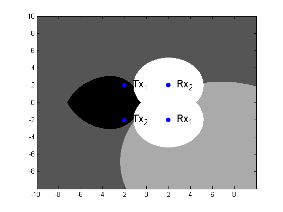
Figure 9: The geographical position in the 2D-plane in which the VSI conditions hold for the ICR subject to phase fading. The black region shows the location of the relay for ICRs without feedback in which DF at the relay achieves capacity at VSI. The union of the black and dark gray regions shows the location of the relay for ICRFs with partial feedback, only from $\mbox{Rx}_{1}$ to the relay, in which DF at the relay achieves capacity at VSI. The union of the black, dark gray and light gray corresponds to ICRF with feedback from both receivers to the relay. The scenario parameters are detailed in Comment 6.

VII-C Comments

Comment 28.

Comparing partial feedback (Corollary 8) with no-feedback [17, Theorem 2], we note that the rate constraints at the destinations are the same. Also note that $\mathbf{a}\in\mathcal{D}_{1}\cap\mathcal{D}_{2}$ guarantees (67a)-(67c), hence as in Comment 5, feedback allows obtaining capacity characterization for a larger set of channel coefficients, and there are scenarios in which feedback strictly enlarges the capacity region (e.g., when $a_{23}$ is very small).

Fig. 9 was created using the same parameters as those used for generating Fig. 2, see Comment 6 for details. The figure demonstrates most clearly the benefits of combining feedback with relaying for interference management. Observe that without feedback, achieving capacity in the VSI regime requires the relay to be close to the transmitters, while partial feedback and moreover full feedback allow achieving capacity for a significantly larger geographical region.

Comment 29.

Note that if we assume a unidirectional noiseless cooperation link from one of the receivers to the other one, then the conditions of the SI and the VSI regime can not be satisfied. Without loss of generality assume a noiseless cooperation link from Rx₁ to Rx₂, then the achievable rate at Rx₂ will always exceed the achievable rate at Rx₁. Hence decoding the interference at Rx₁ will always decrease the capacity region. The same conclusion also holds for decoding both messages at Rx₁. Thus if there is a unidirectional noiseless cooperation link from one of the receivers to the other one, then the SI and the VSI conditions can not be satisfied. Note that this conclusion does not hold for the scenarios where the link between the receivers is noisy or if the receiver first compresses its channel observations prior to forwarding them to the other receiver (see [32] and [33]).

VIII Conclusions

In this paper we characterized the capacity region of the fading interference channel with a relay for different feedback configurations. The capacity region was characterized explicitly for the phase fading and Rayleigh fading scenarios in both SI and VSI regimes. We showed that the capacity is achieved with zero-mean, circularly symmetric complex Normal channel inputs, independent of each other with all transmitters using their maximum available power. It was also shown that when feedback is available at the relay, then the best strategy for the relay in these regimes is to decode both messages and forward them to both receivers and thus assist both receivers simultaneously. We showed that with such a strategy at the relay, when VSI occurs the ICRF behaves like two parallel relay channels. We also showed that when SI occurs, the ICRF behaves like two EMARCs and the same coding strategy achieves capacity for both simultaneously. We next showed that if feedback from both receivers is available at the relay, then additional feedback from each receiver to its opposite transmitter provides no further improvement to the capacity region. However, additional feedback links from each receiver to its corresponding transmitter can enlarge the capacity region. By comparing the scenario where there is partial feedback (from one of the receivers only) or full feedback (from both receivers) at the relay, versus the scenario with no feedback at all, we showed that partial feedback and moreover full feedback increase the range of the channel coefficients which allow achieving capacity in both VSI and SI regimes significantly. With no feedback however, the relay reception must be good in order to achieve capacity (Recall [7, Theorem 6]: in the relay channel under the phase fading assumption, DF achieves capacity when the relay is closer to the source than to the destination).

The fact that the capacity achieving channel inputs are mutually independent allows a relatively simple integration of relaying into existing wireless networks. Also note that since the relay can be optimal for both communicating pairs simultaneously, then a relatively small number of relay stations can optimally assist several nodes simultaneously. These observations support the deployment of relay nodes to assist in managing interference in practical wireless systems such as cellular and WiFi networks. We note however, that additional research, especially on non-fading scenarios is still required to obtain a complete assessment of cost-benefit tradeoff.

Appendix A Maximizing Distribution for the Cut-Set Bound

A-A The Upper Bound on $R_{1}$

Starting with the upper bound on $R_{1}$, we first consider $I(X_{1};Y_{1},Y_{2},Y_{3}|X_{2},X_{3},\underline{\tilde{H}})$. Note that by fixing the side information $\underline{\tilde{H}}=\underline{\tilde{h}}$, we obtain

$$\!\!\!\!\!\!\!\!\!\!\!\!\!\!\!h(Y_{1},Y_{2},Y_{3}|X_{2},X_{3},\underline{\tilde{H}}=\underline{\tilde{h}})$$

$$=h(h_{11}X_{1}+Z_{1},h_{12}X_{1}+Z_{2},$$

$$\qquad\qquad h_{13}X_{1}+Z_{3}|X_{2},X_{3},\underline{\tilde{H}}=\underline{\tilde{h}}).$$ (A.1)

Define $\mathbf{H}\triangleq(H_{11},H_{12},H_{13})^{T},\mathbf{Z}\triangleq(Z_{1},Z_{2},Z_{3})^{T}$. Following these definitions we define ($\hat{Y}_{1},\hat{Y}_{2},\hat{Y}_{3})^{T}\triangleq\mathbf{H}\cdot X_{1}+\mathbf{Z}$. For $\mathbf{X}\triangleq(X_{1},X_{2},X_{3})$, zero-mean, define $\mathds{C}_{1}=\mathds{E}\{\mathbf{X}\mathbf{X}^{H}\}$. Letting $\alpha_{ij}\triangleq\mathds{E}[X_{i}X_{j}^{*}]$ we get

$$\mathds{C}_{1} \triangleq \mathds{E}\left\{\left[\begin{array}[]{c}X_{1}\\ X_{2}\\ X_{3}\end{array}\right][X_{1}^{*},X_{2}^{*},X_{3}^{*}]\right\}$$ (A.5)

$$= \mathds{E}\left\{\left[\begin{array}[]{ccc}X_{1}X_{1}^{*}&X_{1}X_{2}^{*}&X_{1}X_{3}^{*}\\ X_{2}X_{1}^{*}&X_{2}X_{2}^{*}&X_{2}X_{3}^{*}\\ X_{3}X_{1}^{*}&X_{3}X_{2}^{*}&X_{3}X_{3}^{*}\end{array}\right]\right\}$$ (A.9)

$$= \left[\begin{array}[]{ccc}P_{1}&\alpha_{12}&\alpha_{13}\\ \alpha_{21}&P_{2}&\alpha_{23}\\ \alpha_{31}&\alpha_{32}&P_{3}\end{array}\right]$$ (A.13)

$$\triangleq \left[\begin{array}[]{cc}t_{11}&\mathbf{t}_{21}^{H}\\ \mathbf{t}_{21}&\mathds{T}_{22}\end{array}\right],$$ (A.16)

where $t_{11}\triangleq P_{1}$ and $\mathds{T}_{22}$ is $2\times 2$ and p.d.. Next we obtain

$$\!\!\!\!\!\!\!\!\!\!I(X_{1};Y_{1},Y_{2},Y_{3}|X_{2},X_{3},\underline{\tilde{H}})$$ (A.17)

$$= \mathds{E}_{\underline{\tilde{H}}}\bigg{\{}h(Y_{1},Y_{2},Y_{3}|X_{2},X_{3},\underline{\tilde{h}})$$

$$\qquad\qquad\qquad\qquad-h(Y_{1},Y_{2},Y_{3}|X_{1},X_{2},X_{3},\underline{\tilde{h}})\bigg{\}}$$

$$\stackrel{{\scriptstyle(a)}}{{=}} \mathds{E}_{\underline{\tilde{H}}}\bigg{\{}h(\hat{Y}_{1},\hat{Y}_{2},\hat{Y}_{3}|X_{2},X_{3},\underline{\tilde{h}})-h(Z_{1},Z_{2},Z_{3})\bigg{\}}$$

$$\stackrel{{\scriptstyle(b)}}{{\leq}} \mathds{E}_{\underline{\tilde{H}}}\bigg{\{}\log_{2}\Big{(}(\pi e)^{3}\det\big{(}\mbox{cov}(\hat{Y}_{1},\hat{Y}_{2},\hat{Y}_{3}|X_{2},X_{3},\underline{\tilde{h}})\big{)}\Big{)}$$

$$\qquad\qquad\qquad\qquad\qquad\qquad-\log_{2}(\pi e)^{3}\bigg{\}}$$

$$= \mathds{E}_{\underline{\tilde{H}}}\bigg{\{}\log_{2}\Big{(}\det\big{(}\mbox{cov}(\hat{Y}_{1},\hat{Y}_{2},\hat{Y}_{3}|X_{2},X_{3},\underline{\tilde{h}})\big{)}\Big{)}\bigg{\}}$$

$$\stackrel{{\scriptstyle(c)}}{{=}} \mathds{E}_{\underline{\tilde{H}}}\bigg{\{}\log_{2}\Big{(}\det\big{(}\mbox{cov}(\mathbf{H}\cdot X_{1}+\mathbf{Z}|X_{2},X_{3},\underline{\tilde{h}})\big{)}\Big{)}\bigg{\}}$$

$$\stackrel{{\scriptstyle(d)}}{{=}} \mathds{E}_{\underline{\tilde{H}}}\bigg{\{}\log_{2}\Big{(}\det\big{(}\mbox{cov}(\mathbf{H}\cdot X_{1}|X_{2},X_{3},\underline{\tilde{h}})$$

$$\qquad\qquad\qquad\qquad\qquad+\mbox{cov}(\mathbf{Z}|X_{2},X_{3},\underline{\tilde{h}})\big{)}\Big{)}\bigg{\}}$$

$$= \mathds{E}_{\underline{\tilde{H}}}\bigg{\{}\!\log_{2}\Big{(}\!\det\big{(}\mathds{I}+\mathbf{H}\cdot\mbox{cov}(X_{1}|X_{2},X_{3})\cdot\mathbf{H}^{H}\big{)}\Big{)}\!\bigg{\}}$$

$$\stackrel{{\scriptstyle(e)}}{{=}} \mathds{E}_{\underline{\tilde{H}}}\bigg{\{}\!\log_{2}\Big{(}\!\det\big{(}\mathds{I}$$

$$\quad\qquad\qquad+\mathbf{H}\cdot(t_{11}-\mathbf{t}_{21}^{H}\mathds{T}_{22}^{-1}\mathbf{t}_{21})\cdot\mathbf{H}^{H}\big{)}\!\Big{)}\!\bigg{\}}$$

$$\stackrel{{\scriptstyle(f)}}{{=}} \mathds{E}_{\underline{\tilde{H}}}\bigg{\{}\log_{2}\Big{(}\det\big{(}\mathds{I}$$

$$+\mathbf{H}\cdot t_{11}^{\frac{1}{2}}(1-t_{11}^{-\frac{1}{2}}\mathbf{t}_{21}^{H}\mathds{T}_{22}^{-\frac{1}{2}}\mathds{T}_{22}^{-\frac{1}{2}}\mathbf{t}_{21}t_{11}^{-\frac{1}{2}})t_{11}^{\frac{1}{2}}\cdot\mathbf{H}^{H}\big{)}\Big{)}\bigg{\}}$$

$$\stackrel{{\scriptstyle(g)}}{{=}} \mathds{E}_{\underline{\tilde{H}}}\bigg{\{}\!\log_{2}\Big{(}\!\det\big{(}\mathds{I}+\mathbf{H}\cdot t_{11}^{\frac{1}{2}}(1-\mathds{A}\mathds{A}^{H})t_{11}^{\frac{1}{2}}\cdot\mathbf{H}^{H}\big{)}\Big{)}\!\bigg{\}}$$

$$\stackrel{{\scriptstyle(h)}}{{\leq}} \mathds{E}_{\underline{\tilde{H}}}\bigg{\{}\!\log_{2}\Big{(}\!\det\big{(}\mathds{I}+\mathbf{H}\cdot t_{11}^{\frac{1}{2}}\cdot(1-\rho^{2})\cdot t_{11}^{\frac{1}{2}}\cdot\mathbf{H}^{H}\big{)}\Big{)}\!\bigg{\}}$$

$$\stackrel{{\scriptstyle(i)}}{{\leq}} \mathds{E}_{\underline{\tilde{H}}}\bigg{\{}\log_{2}\Big{(}\det\big{(}\mathds{I}+\mathbf{H}\cdot t_{11}\cdot\mathbf{H}^{H}\big{)}\Big{)}\bigg{\}}.$$

Thus, by using [38, Fact 3.7.19], we get the following inequality:

$$\!\!\!\!\!\!\!\!\!\!\!\!\!\!\!\!\!I(X_{1};Y_{1},Y_{2},Y_{3}|X_{2},X_{3},\underline{\tilde{H}})\leq$$

$$\!\!\!\!\!\!\!\!\!\!\!\!\!\!\mathds{E}_{\underline{\tilde{H}}}\bigg{\{}\!\log_{2}\Big{(}1\!+\!P_{1}(|H_{11}|^{2}+|H_{12}|^{2}+|H_{13}|^{2})\Big{)}\!\bigg{\}}.$$ (A.18)

In the above transitions,

• (a) follows from (A-A).

• (b) follows from Lemma 2 which show that $h(\hat{Y}_{1},\hat{Y}_{2},\hat{Y}_{3}|X_{2},X_{3})$ is maximized by jointly circularly symmetric complex Normal RVs with zero mean and same covariance matrix as $(\hat{Y}_{1},\hat{Y}_{2},\hat{Y}_{3},X_{2},X_{3})$.

• (c) follows from the definition of $\hat{Y}_{1},\hat{Y}_{2},\hat{Y}_{3},\mathbf{H}$ and $\mathbf{Z}$.

• (d) follows from the fact that $\mathbf{Z}$ is independent of $X_{k},k\in\{1,2,3\}$.

• (e) follows from [35, Sec. VI] which shows that the conditional covariance matrix of jointly complex normal RVs is given by the Schur complement of $\mathds{T}_{22}$ in the covariance matrix $\mathds{C}_{1}$.

• (f) follows from [38, Proposition 8.1.2 and Lemma 8.2.1].

• (g) follows from the definition $\mathds{A}\triangleq t_{11}^{-\frac{1}{2}}\mathbf{t}_{21}^{H}\mathds{T}_{22}^{-\frac{1}{2}}$.

• (h) follows from [46, Lemma 3.1] and from [37, Theorem 7.7.2 and Theorem 7.7.4].

• (i) follows from the range of $\rho$, as given in [46, Lemma 3.1]: $\rho\in[0,1]$ and from [37, Theorem 7.7.2 and Theorem 7.7.4] which state that since $(1-\rho^{2})t_{11}\leq t_{11}$ then $\det(\mathds{I}+\mathbf{H}(1-\rho^{2})t_{11}\mathbf{H}^{H})\leq\det(\mathds{I}+\mathbf{H}t_{11}\mathbf{h}^{H})$.

Next, note that (A.18) does not depend on $\alpha_{12},\alpha_{13}$ or $\alpha_{23}$ and it can be achieved with equality from (A.17) by setting $\alpha_{12}=\alpha_{13}=0$, irrespective of the value of $\alpha_{23}$, which can also be set to zero. We also note that since $\log_{2}(x)$ monotonically increases with respect to $x$, then $I(X_{1};Y_{1},Y_{2},Y_{3}|X_{2},X_{3},\underline{\tilde{H}})$ is maximized when Tx₁ transmits at its maximum available power. Finally, (b) is achieved with equality if $X_{1},X_{2},X_{3}$ are jointly Normal. As these variables are uncorrelated, they are also independent. In conclusion, $I(X_{1};Y_{1},Y_{2},Y_{3}|X_{2},X_{3},\underline{\tilde{H}})$ is maximized by mutually independent, circularly symmetric complex Normal channel inputs with zero mean.

Next we consider $I(X_{1},X_{3};Y_{1}|X_{2},\tilde{H}_{1})$. Following the same arguments as the previous rate bound, note that

$$\!\!\!\!\!\!\!\!\!\!\!\!\!\!\!h(Y_{1}|X_{2},\tilde{H}_{1}=\tilde{h}_{1})$$

$$\;\;=h(h_{11}X_{1}+h_{31}X_{3}+Z_{1}|X_{2},\tilde{H}_{1}=\tilde{h}_{1}).$$ (A.19)

Define

$$\hat{Y}_{1} \triangleq H_{11}X_{1}+H_{31}X_{3}+Z_{1},$$ (A.20a)

$$\mathds{C}_{2} \triangleq \mathds{E}\left\{\left[\begin{array}[]{c}\hat{Y}_{1}\\ X_{2}\end{array}\right]\left[\begin{array}[]{cc}\hat{Y}_{1}^{*},X_{2}^{*}\end{array}\right]\Bigg{|}\tilde{H}_{1}\right\}$$ (A.20e)

$$= \mathds{E}\left\{\left[\begin{array}[]{cc}\hat{Y}_{1}\hat{Y}_{1}^{*}&\hat{Y}_{1}X_{2}^{*}\\ X_{2}\hat{Y}_{1}^{*}&X_{2}X_{2}^{*}\end{array}\right]\Bigg{|}\tilde{H}_{1}\right\}$$ (A.20h)

$$= \left[\begin{array}[]{cc}T_{11}&T_{12}\\ T_{12}^{*}&t_{22}\end{array}\right].$$ (A.20k)

Hence, we bound $I(X_{1},X_{3};Y_{1}|X_{2},\tilde{H}_{1})$ as follows:

$$\!\!\!\!\!\!\!\!\!\!\!\!\!\!\!I(X_{1},X_{3};Y_{1}|X_{2},\tilde{H}_{1})$$

$$= \mathds{E}_{\tilde{H}_{1}}\bigg{\{}h(Y_{1}|X_{2},\tilde{h}_{1})-h(Y_{1}|X_{1},X_{2},X_{3},\tilde{h}_{1})\bigg{\}}$$

$$\stackrel{{\scriptstyle(a)}}{{\leq}} \mathds{E}_{\tilde{H}_{1}}\bigg{\{}\log_{2}\Big{(}\det\big{(}\mbox{cov}(\hat{Y}_{1}|X_{2},\tilde{h}_{1})\big{)}\Big{)}\bigg{\}}$$

$$= \mathds{E}_{\tilde{H}_{1}}\bigg{\{}\log_{2}\Big{(}T_{11}-T_{12}t_{22}^{-1}T_{12}^{*}\Big{)}\bigg{\}}$$

$$\stackrel{{\scriptstyle(b)}}{{\leq}} \mathds{E}_{\tilde{H}_{1}}\bigg{\{}\log_{2}\Big{(}T_{11}\Big{)}\bigg{\}}.$$

Thus, we get

$$\!\!\!\!I(X_{1},X_{3};Y_{1}|X_{2},\tilde{H}_{1})$$

$$\leq\mathds{E}_{\tilde{H}_{1}}\Big{\{}\log_{2}(|H_{11}|^{2}P_{1}+H_{11}H_{31}^{*}\alpha_{13}$$

$$\qquad\qquad\qquad+H_{31}H_{11}^{*}\alpha_{31}+|H_{31}|^{2}P_{3}+1)\Big{\}}.\phantom{xxxx}$$ (A.22)

Here, (a) follows from the definition of $\hat{Y}_{1}$ in (A.20a), from (A-A) and from Lemma 2, and (b) follows from the fact that $T_{12}^{*}T_{12}=|T_{12}|^{2}\geq 0$. Next, note that:

$$\!\!\!\!\mathds{E}_{\tilde{H}_{1}}\Big{\{}\log_{2}(T_{11})\Big{\}}$$

$$=\int_{\tilde{h}_{1}\in\mathfrak{C}^{3}}\!\!\!\!\!\!\log_{2}\big{(}|h_{11}|^{2}P_{1}+h_{11}h_{31}^{*}\alpha_{13}+h_{31}h_{11}^{*}\alpha_{31}$$

$$\qquad\qquad\qquad\qquad\quad+|h_{31}|^{2}P_{3}+1\big{)}f_{\tilde{H}_{1}}(\tilde{h}_{1})d\tilde{h}_{1}.$$

Hence, if we replace $H_{31}$ with $-H_{31}$, the result of the integral remains unchanged. This follows as $h_{ij}$’s are independent complex RVs with uniform phases on $[0,2\pi)$, independent of their magnitudes, and therefore the value of the integration is the same for all initial phases. Hence, following the same technique as in [7, Theorem 8] and from concavity of the logarithm function, we can apply Jensen’s inequality and rewrite the bound in (A-A) as:

$$\!\!\!\!\!\!\!\!\!\!\!\!\!\!\!\!\!\!\!I(X_{1},X_{3};Y_{1}|X_{2},\tilde{H}_{1})\leq\mathds{E}_{\tilde{H}_{1}}\Big{\{}\log_{2}(T_{11})\Big{\}}$$

$$\!\!\!\!\!\!\!\!\leq\mathds{E}_{\tilde{H}_{1}}\Big{\{}\log_{2}(|H_{11}|^{2}P_{1}+|H_{31}|^{2}P_{3}+1)\Big{\}}.$$ (A.23)

As the bound in (A-A) does not depend on $\alpha_{12},\alpha_{13}$ or $\alpha_{23}$, then (A-A) is achieved with equality from (A-A) by setting $\alpha_{12}=\alpha_{13}=\alpha_{23}=0$.

We conclude that the upper bound on $R_{1}$ in cut-set bound is maximized by mutually independent, zero-mean, circularly symmetric complex Normal channel inputs, and with all sources transmitting at their maximum available power.

A-B The Upper Bound on $R_{2}$

Following steps similar to those in section A-A, we conclude that the mutual expressions $I(X_{2};Y_{1},Y_{2},Y_{3}|X_{1},X_{3},\underline{\tilde{H}})$ and $I(X_{2},X_{3};Y_{2}|X_{1},\tilde{H}_{2})$ are both maximized by mutually independent, zero mean, circularly symmetric complex Normal channel inputs.

A-C The Upper Bound on $R_{1}+R_{2}$

First, note that

$$h(Y_{1},Y_{2},Y_{3}|X_{3},\underline{\tilde{H}}=\tilde{\underline{h}})=$$

$$\qquad h\big{(}h_{11}X_{1}+h_{21}X_{2}+Z_{1},h_{12}X_{1}+h_{22}X_{2}+Z_{2},$$

$$\qquad\quad\quad h_{13}X_{1}+h_{23}X_{2}+Z_{3}|X_{3},\underline{\tilde{H}}=\tilde{\underline{h}}).$$ (A.24)

Define $\mathds{H},\mathbf{X},\mathbf{Z}$ and rewrite $\mathds{C}_{1}$ from (A.5) as

$$\mathds{H} \triangleq \left[\begin{array}[]{cc}H_{11}&H_{21}\\ H_{12}&H_{22}\\ H_{13}&H_{23}\end{array}\right]$$ (A.25d)

$$\mathbf{X} \triangleq \left[\begin{array}[]{c}X_{1}\\ X_{2}\end{array}\right]$$ (A.25g)

$$\mathbf{Z} \triangleq \left[\begin{array}[]{c}Z_{1}\\ Z_{2}\\ Z_{3}\end{array}\right]$$ (A.25k)

$$\mathds{C}_{1} \triangleq \left[\begin{array}[]{cc}\mathds{T}_{11}&\mathbf{t}_{12}\\ \mathbf{t}_{12}^{H}&t_{22}\end{array}\right],$$ (A.25n)

where $\mathds{T}_{11}$ is $2\times 2$ and p.d. and $t_{22}\triangleq P_{3}$. Using the above definitions we obtain

$$\!\!\!\!\!\!\!\!\!\!\!\!\!\!\!\!\!\!\!\!I(X_{1},X_{2};Y_{1},Y_{2},Y_{3}|X_{3},\underline{\tilde{H}})$$ (A.26)

$$= \mathds{E}_{\underline{\tilde{H}}}\bigg{\{}h(Y_{1},Y_{2},Y_{3}|X_{3},\underline{\tilde{h}})$$

$$\qquad\qquad-h(Y_{1},Y_{2},Y_{3}|X_{1},X_{2},X_{3},\underline{\tilde{h}})\bigg{\}}$$

$$\leq \mathds{E}_{\underline{\tilde{H}}}\bigg{\{}\log_{2}\Big{(}\det\big{(}\mathds{I}+\mathds{H}\cdot(\mathds{T}_{11}$$

$$\qquad\qquad\qquad-\mathbf{t}_{12}t_{22}^{-1}\mathbf{t}_{12}^{H})\cdot\mathds{H}^{H}\big{)}\Big{)}\bigg{\}}$$

$$\stackrel{{\scriptstyle(a)}}{{\leq}} \mathds{E}_{\underline{\tilde{H}}}\bigg{\{}\log_{2}\Big{(}\det\big{(}\mathds{I}+\mathds{H}\cdot\mathds{T}_{11}\cdot\mathds{H}^{H}\big{)}\Big{)}\bigg{\}}.$$ (A.27)

Thus, we bound $I(X_{1},X_{2};Y_{1},Y_{2},Y_{3}|X_{3},\underline{\tilde{H}})$ as follows:

$$\!\!\!\!I(X_{1},X_{2};Y_{1},Y_{2},Y_{3}|X_{3},\underline{\tilde{H}})$$

$$\leq\mathds{E}_{\underline{\tilde{H}}}\bigg{\{}\log_{2}\Big{(}1+\big{(}\sum_{i=1}^{2}P_{i}(|H_{i1}|^{2}+|H_{i2}|^{2}+|H_{i3}|^{2})\big{)}$$

$$\qquad+\big{(}(P_{1}P_{2}-|\alpha_{12}|^{2})(|H_{11}|^{2}|H_{22}|^{2}+|H_{11}|^{2}|H_{23}|^{2}$$

$$\qquad+|H_{12}|^{2}|H_{21}|^{2}+|H_{12}|^{2}|H_{23}|^{2}+|H_{13}|^{2}|H_{21}|^{2}$$

$$\qquad+|H_{13}|^{2}|H_{22}|^{2}-2V_{1}-2V_{2}-2V_{3})\big{)}$$

$$\qquad+\alpha_{12}\big{(}H_{11}H_{21}^{*}+H_{12}H_{22}^{*}+H_{13}H_{23}^{*}\big{)}$$

$$\qquad+\alpha_{21}\big{(}H_{21}H_{11}^{*}+H_{22}H_{12}^{*}+H_{23}H_{13}^{*}\big{)}\Big{)}\bigg{\}},$$ (A.28)

where

$$V_{1} = \mathfrak{Re}\{H_{11}H_{22}H_{12}^{*}H_{21}^{*}\}$$ (A.29a)

$$V_{2} = \mathfrak{Re}\{H_{12}H_{23}H_{13}^{*}H_{22}^{*}\}$$ (A.29b)

$$V_{3} = \mathfrak{Re}\{H_{13}H_{21}H_{11}^{*}H_{23}^{*}\}.$$ (A.29c)

The transitions used in the above derivation are similar to those used in section A-A. Here, (a) follows from [46, Lemma 3.1] and from [37, Theorem 7.7.2]. Following the same technique as in [7, Theorem 8] we obtain that replacing $H_{11},H_{12},H_{13}$ with $-H_{11},-H_{12},-H_{13}$, respectively, does not change the expected value in (A-C). This is equivalent to replacing $\alpha_{12}$ and $\alpha_{21}$ with $-\alpha_{12}$ and $-\alpha_{21}$. The above observation can be used to express (A-C) as:

$$\!\!\!\!\!\!\!\!\!\!\mathds{E}_{\underline{\tilde{H}}}\bigg{\{}\log_{2}\Big{(}\det\big{(}\mathds{I}+\mathds{H}\mathds{T}_{11}\mathds{H}^{H}\big{)}\Big{)}\bigg{\}}$$ (A.30)

$$\stackrel{{\scriptstyle(a)}}{{\leq}} \mathds{E}_{\underline{\tilde{H}}}\bigg{\{}\log_{2}\Big{(}1+\big{(}\sum_{i=1}^{2}P_{i}(|H_{i1}|^{2}+|H_{i2}|^{2}+|H_{i3}|^{2})\big{)}$$

$$\quad+\big{(}(P_{1}P_{2}-2|\alpha_{12}|^{2})(|H_{11}|^{2}|H_{22}|^{2}$$

$$\quad\quad+|H_{11}|^{2}|H_{23}|^{2}+|H_{12}|^{2}|H_{21}|^{2}$$

$$\quad\quad+|H_{12}|^{2}|H_{23}|^{2}+|H_{13}|^{2}|H_{21}|^{2}$$

$$\quad\quad+|H_{13}|^{2}|H_{22}|^{2}-2V_{1}-2V_{2}-2V_{3})\big{)}\!\Big{)}\!\bigg{\}},$$

where (a) follows from the concavity of the logarithm function. Next, we have the following proposition:

Proposition A.1.

The expression in (A.30) is maximized when $\alpha_{12}=0$ and when Tx₁ and Tx₂ transmit at their maximum available power, i.e.,

$$\!\!\!\!\mathds{E}_{\underline{\tilde{H}}}\bigg{\{}\log_{2}\Big{(}\det\big{(}\mathds{I}+\mathds{H}\mathds{T}_{11}\mathds{H}^{H}\big{)}\Big{)}\bigg{\}}\leq$$

$$\;\mathds{E}_{\underline{\tilde{H}}}\bigg{\{}\log_{2}\Big{(}1+\big{(}\sum_{i=1}^{2}P_{i}(|H_{i1}|^{2}+|H_{i2}|^{2}+|H_{i3}|^{2})\big{)}$$

$$\qquad\quad+P_{1}P_{2}\big{(}|H_{11}|^{2}|H_{22}|^{2}+|H_{11}|^{2}|H_{23}|^{2}$$

$$\qquad\quad+|H_{12}|^{2}|H_{21}|^{2}+|H_{12}|^{2}|H_{23}|^{2}+|H_{13}|^{2}|H_{21}|^{2}$$

$$\qquad\quad+|H_{13}|^{2}|H_{22}|^{2}-2V_{1}-2V_{2}-2V_{3}\big{)}\Big{)}\!\bigg{\}},$$ (A.31)

where $V_{1},V_{2},V_{3}$ are defined in (A.29).

Proof.

Consider $H_{11},H_{22},H_{12},H_{21}\in\mathcal{C}$ and $V_{1},V_{2},V_{3}$ as defined in (A.29). Without loss of generality, we can write:

$$H_{11}H_{22} = A+Bi$$

$$H_{12}H_{21} = C+Di,$$

$A,B,C,D\in\mathcal{R}$. Using the above definitions we get: $2V_{1}=2\cdot\mathfrak{Re}\{H_{11}H_{22}H_{12}^{*}H_{21}^{*}\}=2(AC+BD)$. Also note that: $A^{2}+C^{2}\geq 2AC$ for all $A,C\in\mathcal{R}$. Thus

$$|H_{11}|^{2}|H_{22}|^{2}+|H_{12}|^{2}|H_{21}|^{2} \geq 2\cdot\mathfrak{Re}\{H_{11}H_{22}H_{12}^{*}H_{21}^{*}\}$$

$$= 2V_{1}.$$

Repeating this argument for $V_{2}$ and $V_{3}$, we conclude that the multiplier of $(P_{1}P_{2}-2|\alpha_{12}|^{2})$ in (A.30) is non-negative and omitting $2|\alpha_{12}|^{2}$ from (A.30) does not reduce the expected value. This leads to (A.1). Also note that since $\log(x)$ monotonically increases with respect to $x$, then (A.1) is maximized when Tx₁ and Tx₂ transmit at their maximum available power. ∎

Hence, (A.1) can be obtained with equality from (A.26) by setting $\alpha_{12}=\alpha_{13}=\alpha_{23}=0$. We conclude that the mutual information expressions in the cut-set bound are maximized by zero-mean, complex Normal channel inputs independent of each other, and with all sources transmitting at their maximum available power.

Appendix B The Capacity Region of the EMARC

The capacity of the EMARC is stated in the following theorem:

Theorem B.1.

Consider the fading EMARC with Rx-CSI derived from the ICRF, given by equations (1) where its message destination is Rx₁ but the relay receives feedback from both receivers s.t. $y_{1,1}^{i-1},y_{2,1}^{i-1},\tilde{h}_{1,1}^{i-1}$ and $\tilde{h}_{2,1}^{i-1}$ are available at the relay at time $i$, prior to transmission. Assume that the channel coefficients are independent in time and independent of each other s.t. their phases are i.i.d. and distributed uniformly over $[0,2\pi)$. Let the additive noises be i.i.d. circularly symmetric complex Normal processes, $\mathcal{CN}(0,1)$, and let the sources have power constraints $\mathds{E}\big{\{}|X_{k}|^{2}\big{\}}\leq P_{k}$, $k\in\{1,2,3\}$. The capacity region is then given by all nonnegative rate pairs s.t.

$$R_{1} \leq \min\{I(X_{1};Y_{1},Y_{2},Y_{3}|X_{2},X_{3},\underline{\tilde{H}}),$$ (B.1a)

$$\qquad\qquad I(X_{1},X_{3};Y_{1}|X_{2},\tilde{H}_{1})\}$$

$$R_{2} \leq \min\{I(X_{2};Y_{1},Y_{2},Y_{3}|X_{1},X_{3},\underline{\tilde{H}}),$$ (B.1b)

$$\qquad I(X_{2},X_{3};Y_{1}|X_{1},\tilde{H}_{1})\}$$

$$R_{1}+R_{2} \leq \min\{I(X_{1},X_{2};Y_{1},Y_{2},Y_{3}|X_{3},\underline{\tilde{H}}),$$ (B.1c)

$$\qquad I(X_{1},X_{2},X_{3};Y_{1}|\tilde{H}_{1})\},$$

and it is achieved with $X_{k}\sim\mathcal{CN}(0,P_{k}),k\in\{1,2,3\}$, mutually independent and with DF strategy at the relay.

Proof.

The proof consists of the following steps:

• We provide an outer bound on the capacity region using the cut-set bound.

• We show that the input distribution that maximizes the outer bound is zero-mean, circularly symmetric complex Normal with channel inputs independent of each other and with maximum allowed power.

• Assuming codebooks generated according to the maximizing distribution, we present an achievable rate region using the DF strategy at the relay:

  • For decoding at the relay, we follow steps similar to [7, Sec. 4.D].

  • We provide an achievable rate region for decoding at the destination by considering a backward decoding scheme.

• We conclude that the intersection of the achievable rate regions for decoding at the relay and at the destination coincides with the cut-set bound.

B-A An Outer Bound

The following bounds are the cut-set bounds of the EMARC rate region:

$$\mathcal{S} \triangleq \{\mbox{Tx}_{1}\},\mathcal{S}^{C}\triangleq\{\mbox{Tx}_{2},\mbox{Relay},\mbox{Rx}_{1},\mbox{Rx}_{2}\}:\phantom{xxxxxx}$$ (B.2a)

$$\quad R_{1}\leq I(X_{1};Y_{1},Y_{2},Y_{3}|X_{2},X_{3},\underline{\tilde{H}})$$

$$\mathcal{S} \triangleq \{\mbox{Tx}_{1},\mbox{Relay},\mbox{Rx}_{2}\},\mathcal{S}^{C}\triangleq\{\mbox{Tx}_{2},\mbox{Rx}_{1}\}:\phantom{xxxxxx}$$ (B.2b)

$$\quad R_{1}\leq I(X_{1},X_{3};Y_{1}|X_{2},\tilde{H}_{1})$$

$$\mathcal{S} \triangleq \{\mbox{Tx}_{2}\},\mathcal{S}^{C}\triangleq\{\mbox{Tx}_{1},\mbox{Relay},\mbox{Rx}_{1},\mbox{Rx}_{2}\}:\phantom{xxxxxx}$$ (B.2c)

$$\quad R_{2}\leq I(X_{2};Y_{1},Y_{2},Y_{3}|X_{1},X_{3},\underline{\tilde{H}})$$

$$\mathcal{S} \triangleq \{\mbox{Tx}_{2},\mbox{Relay},\mbox{Rx}_{1}\},\mathcal{S}^{C}\triangleq\{\mbox{Tx}_{1},\mbox{Rx}_{2}\}:\phantom{xxxxxx}$$ (B.2d)

$$\quad R_{2}\leq I(X_{2},X_{3};Y_{1}|X_{1},\tilde{H}_{2})$$

$$\mathcal{S} \triangleq \{\mbox{Tx}_{1},\mbox{Tx}_{2}\},\mathcal{S}^{C}\triangleq\{\mbox{Rx}_{1},\mbox{Rx}_{2},\mbox{Relay}\}:\phantom{xxxxxx}$$ (B.2e)

$$\quad R_{1}+R_{2}\leq I(X_{1},X_{2};Y_{1},Y_{2},Y_{3}|X_{3},\underline{\tilde{H}})$$

$$\mathcal{S} \triangleq \{\mbox{Tx}_{1},\mbox{Tx}_{2},\mbox{Relay},\mbox{Rx}_{2}\},\mathcal{S}^{C}\triangleq\{\mbox{Rx}_{1}\}:\phantom{xxxxxx}$$ (B.2f)

$$\quad R_{1}+R_{2}\leq I(X_{1},X_{2},X_{3};Y_{1}|\underline{\tilde{H}}).$$

Following the same arguments as in sections A-A, A-B and A-C we conclude that the outer bounds on $R_{1}$ and $R_{2}$ are maximized by mutually independent, zero-mean, circularly symmetric complex Normal channel inputs and with all sources transmitting at their maximum available power. Moreover, we obtain an upper bound on $I(X_{1},X_{2},X_{3};Y_{1}|\tilde{H}_{1})$:

$$\!\!\!\!\!\!\!\!\!\!\!\!I(X_{1},X_{2},X_{3};Y_{1}|\tilde{H}_{1})$$

$$\!\!\!\!\!\!\!\!\!\!\!\!\leq\mathds{E}_{\tilde{H}_{1}}\!\bigg{\{}\!\!\log_{2}\Big{(}\!1\!+\!|H_{11}|^{2}P_{1}\!+\!|H_{21}|^{2}P_{2}\!+\!|H_{31}|^{2}P_{3}\Big{)}\!\!\bigg{\}},$$ (B.3)

and we conclude that it is achieved by mutually independent, zero mean, circularly symmetric complex Normal channel inputs.

B-B An Achievable Rate Region

The achievability is based on DF strategy at the relay. Fix the block length $n$ and the input distributions: $f_{X_{1}}(x_{1}),f_{X_{2}}(x_{2}),f_{X_{3}}(x_{3})$ where $f_{X_{k}}(x_{k})\sim\mathcal{CN}(0,P_{k}),k\in\{1,2,3\}$. The following encoding and decoding methods are considered:

B-B1 Code Construction

The code construction is similar to section IV-A2.

B-B2 Encoding at Block b

The encoding process is similar to section IV-A2.

B-B3 Decoding at the Relay at Block b

The decoding process at the relay is similar to Section IV-A2, leading to the rate constraints (7).

B-B4 Decoding at the Destination

The receiver uses a backward block decoding method. Assume that the receiver has successfully decoded $m_{1,b+1}$ and $m_{2,b+1}$. Then

• In the first step the receiver generates the sets:

  $$\!\!\!\!\!\!\!\!\mathcal{E}_{0,b} \triangleq \Big{\{}(m_{1},m_{2})\in\mathcal{M}_{1}\times\mathcal{M}_{2}:\big{(}\mathbf{x}_{1}(m_{1,b+1}),$$

  $$\!\!\!\!\!\!\!\!\!\!\!\!\!\!\!\!\!\!\!\!\mathbf{x}_{2}(m_{2,b+1}),\mathbf{x}_{3}(m_{1},m_{2}),\mathbf{y}_{1}(b+1),\mathbf{\tilde{h}}_{1}(b+1)\big{)}\!\!\in\!\!A_{\epsilon}^{(n)}\Big{\}}.$$

  $$\!\!\!\!\!\!\!\!\mathcal{E}_{1,b} \triangleq \Big{\{}(m_{1},m_{2})\in\mathcal{M}_{1}\times\mathcal{M}_{2}:\big{(}\mathbf{x}_{1}(m_{1}),$$

  $$\qquad\qquad\mathbf{x}_{2}(m_{2}),\mathbf{y}_{1}(b),\mathbf{\tilde{h}}_{1}(b)\big{)}\in A_{\epsilon}^{(n)}\Big{\}}.$$

• The receiver then decodes $(m_{1,b},m_{2,b})$ by finding a unique pair $(m_{1},m_{2})\in\mathcal{E}_{0,b}\cap\mathcal{E}_{1,b}$.

Let the decoded pair be $(\hat{m}_{1,b},\hat{m}_{2,b})$. A decoding error happens if one of the following error events, associated with the decoding rule at the destination occurs:

• $E_{0,b}\cup E_{1,b}$, where

  $$\!\!\!\!\!\!\!\!E_{0,b} \triangleq \Big{\{}\big{(}\mathbf{x}_{1}(m_{1,b+1}),\mathbf{x}_{2}(m_{2,b+1}),\mathbf{x}_{3}(m_{1,b},m_{2,b}),$$

  $$\qquad\qquad\qquad\mathbf{y}_{1}(b+1),\mathbf{\tilde{h}}_{1}(b+1)\big{)}\notin A_{\epsilon}^{(n)}\Big{\}}$$

  $$\!\!\!\!\!\!\!\!E_{1,b} \triangleq \Big{\{}\big{(}\mathbf{x}_{1}(m_{1,b}),\mathbf{x}_{2}(m_{2,b}),\mathbf{y}_{1}(b),\mathbf{\tilde{h}}_{1}(b)\big{)}\notin A_{\epsilon}^{(n)}\Big{\}}.$$

  From joint-typicality, the probability of the above event can be arbitrarily small if $n$ is large enough.

• $E_{2,b}\triangleq\big{\{}(\hat{m}_{1,b}\neq m_{1,b},m_{2,b})\in\mathcal{E}_{0,b}\cap\mathcal{E}_{1,b}\big{\}}$. From [6, Lemma 2]:

  $$\!\!\!\!\!\!\Pr\{(\hat{m}_{1,b}\neq m_{1,b},m_{2,b})\in\mathcal{E}_{0,b}\}$$

  $$\qquad\qquad\qquad\qquad\leq 2^{-n(I(X_{3};Y_{1}|X_{1},X_{2},\tilde{H}_{1})-7\epsilon)}$$

  $$\!\!\!\!\!\!\Pr\{(\hat{m}_{1,b}\neq m_{1,b},m_{2,b})\in\mathcal{E}_{1,b}\}$$

  $$\qquad\qquad\qquad\qquad\leq 2^{-n(I(X_{1};Y_{1}|X_{2},\tilde{H}_{1})-7\epsilon)}.$$

  Note that since the codebooks are constructed independent of each other then $\mathcal{E}_{0,b}$ is independent of $\mathcal{E}_{1,b}$ and the probability of $E_{2,b}$ can be arbitrarily small if $n$ is large enough and

  $$R_{1} \leq I(X_{3};Y_{1}|X_{1},X_{2},\tilde{H}_{1})+I(X_{1};Y_{1}|X_{2},\tilde{H}_{1})$$ (B.4a)

  $$= I(X_{1},X_{3};Y_{1}|X_{2},\tilde{H}_{1}).$$

• $E_{3,b}\triangleq\big{\{}(m_{1,b},\hat{m}_{2,b}\neq m_{2,b})\in\mathcal{E}_{0,b}\cap\mathcal{E}_{1,b}\big{\}}$. From [6, Lemma 2], the probability of this event can be arbitrarily small if $n$ is large enough and

  $$R_{2}\leq I(X_{2},X_{3};Y_{1}|X_{1},\tilde{H}_{1}).$$ (B.4b)

• $E_{4,b}\triangleq\big{\{}(\hat{m}_{1,b}\neq m_{1,b},\hat{m}_{2,b}\neq m_{2,b})\in\mathcal{E}_{0,b}\cap\mathcal{E}_{1,b}\big{\}}$. From [6, Lemma 2]:

  $$\!\!\!\!\!\Pr\{(\hat{m}_{1,b}\neq m_{1,b},\hat{m}_{2,b}\neq m_{2,b})\in\mathcal{E}_{0,b}\}$$

  $$\qquad\qquad\qquad\qquad\leq 2^{-n\big{(}I(X_{3};Y_{1}|X_{1},X_{2},\tilde{H}_{1})-7\epsilon\big{)}}$$

  $$\!\!\!\!\!\Pr\{(\hat{m}_{1,b}\neq m_{1,b},\hat{m}_{2,b}\neq m_{2,b})\in\mathcal{E}_{1,b}\}$$

  $$\qquad\qquad\qquad\qquad\leq 2^{-n\big{(}I(X_{1},X_{2};Y_{1}|\tilde{H}_{1})-7\epsilon\big{)}},$$

  the probability of this event can be arbitrarily small if $n$ is large enough and

  $$\!\!\!\!\!\!\!\!\!\!R_{1}+R_{2} \leq I(X_{3};Y_{1}|X_{1},X_{2},\tilde{H}_{1})+I(X_{1},X_{2};Y_{1}|\tilde{H}_{1})$$ (B.4c)

  $$= I(X_{1},X_{2},X_{3};Y_{1}|\tilde{H}_{1}).$$

Combining (7) and (B.4), we obtain the achievable rate region of the EMARC:

$$\!\!\!\!\!\!\!\!\!\!\!\!\mathcal{R}_{\scriptsize{\mbox{EMARC}}}$$

$$\!\!\!\!\!\!=\bigg{\{}(R_{1},R_{2})\in\mathfrak{R}^{2}_{+}:$$

$$R_{1}\leq\min\big{\{}I(X_{1};Y_{1},Y_{2},Y_{3}|X_{2},X_{3},\underline{\tilde{H}}),$$

$$\qquad\qquad\qquad\quad\;I(X_{1},X_{3};Y_{1}|X_{2},\tilde{H}_{1})\big{\}}$$ (B.5a)

$$R_{2}\leq\min\big{\{}I(X_{2};Y_{1},Y_{2},Y_{3}|X_{2},X_{3},\underline{\tilde{H}}),$$

$$\qquad\qquad\qquad\quad\;I(X_{2},X_{3};Y_{1}|X_{1},\tilde{H}_{1})\big{\}}$$ (B.5b)

$$R_{1}+R_{2}\leq\min\big{\{}I(X_{1},X_{2};Y_{1},Y_{2},Y_{3}|X_{3},\underline{\tilde{H}}),$$

$$\qquad\qquad\qquad\quad\;I(X_{1},X_{2},X_{3};Y_{1}|\tilde{H}_{1})\big{\}}\bigg{\}}.$$ (B.5c)

Finally, note that (B.5) coincides with the cut-set bound in (B.2) and thus it is the capacity region of the EMARC. ∎

Appendix C Proof of Proposition 3

Inner bound

: Note that the region $\tilde{\mathcal{R}}_{ICRF}^{VSI}$ can be obtained by time-sharing between two rate points: point $A$ is the rate pair $(R_{1,A},R_{2,A})=\big{(}I(X_{1},X_{3};Y_{1}|X_{2},\tilde{H}_{1}),I(X_{2},X_{3};Y_{2}|X_{1},\tilde{H}_{2})\big{)}$, and point $B$ is the rate pair $(R_{1,B},R_{2,B})=\big{(}I(X_{1},X_{2},X_{3};Y_{1}|\tilde{H}_{1}),0\big{)}$. Theorem 1 shows that in the VSI regime $(R_{1,A},R_{2,A})$ is achievable. We next show that $(R_{1,B},R_{2,B})$ is achievable. This is done using the DF-based achievability scheme described in the following:

Fix the blocklength $n$ and the input distribution $f_{X_{1},X_{2},X_{3}}(x_{1},x_{2},x_{3})=f_{X_{1}}(x_{1})\cdot f_{X_{2}}(x_{2})\cdot f_{X_{3}}(x_{3})$ where $X_{k}\sim\mathcal{CN}(0,P_{k})\mbox{ }k\in\{1,2,3\}$. Note that as $R_{2}=0$, then $\mbox{Tx}_{2}$ acts as a second relay for sending $m_{1}$ from $\mbox{Tx}_{1}$ to $\mbox{Rx}_{1}$. We use $nB$ channel symbols for sending $B-1$ messages.

Codebook Construction

For each $m_{1}\in\mathcal{M}_{1}$ and $k\in\{1,2,3\}$, select a codeword $\mathbf{x}_{k}(m_{1})$ according to the p.d.f. $f_{\mathbf{X}_{k}}\big{(}\mathbf{x}_{k}(m_{1})\big{)}=\prod_{i=1}^{n}f_{X_{k}}\big{(}x_{k,i}(m_{1})\big{)}$.

Encoding at Block $b$

At block $b$, Tx₁ transmits $m_{1,b}$ using $\mathbf{x}_{1}(m_{1,b})$. Let $\hat{m}_{1,b-1},\hat{\hat{m}}_{1,b-1}$ denote the decoded $m_{1,b-1}$ at the end of block $b-1$, at the relay and at Tx₂, respectively. At block $b$, Tx₂ transmits $\mathbf{x}_{2}(\hat{\hat{m}}_{1,b-1})$ and the relay transmits $\mathbf{x}_{3}(\hat{m}_{1,b-1})$. At block $b=1$, Tx₂ transmits $\mathbf{x}_{2}(1)$, and the relay transmits $\mathbf{x}_{3}(1)$, and at block $b=B$, Tx₁ transmits $\mathbf{x}_{1}(1)$.

Decoding at the Relay and at Tx₂ at Block $b$

The relay and $\mbox{Tx}_{2}$ each uses a joint-typicality decoder. We now find conditions for bounding the average probability of error averaged over all codebooks. The decoder at the relay looks for a unique $m_{1}\in\mathcal{M}_{1}$ which satisfies

$$\Big{(}\mathbf{x}_{1}(m_{1}),\mathbf{x}_{2}(m_{1,b-1}),\mathbf{x}_{3}(m_{1,b-1}),\mathbf{y}_{1}(b),\mathbf{y}_{2}(b),$$

$$\qquad\mathbf{y}_{3}(b),\mathbf{\underline{\tilde{h}}}(b)\Big{)}\in A_{\epsilon}^{(n)}(X_{1},X_{2},X_{3},Y_{1},Y_{2},Y_{3},\underline{\tilde{H}}).$$

We conclude that the relay can decode $m_{1,b}$ with an arbitrarily small probability of error if $n$ is large enough and

$$R_{1}<I(X_{1};Y_{1},Y_{2},Y_{3}|X_{2},X_{3},\underline{\tilde{H}}).$$ (C.1a)

Following the same approach, we can show that $$\mbox{Tx}_{2} m_{1,b} n$$ can decode reliably if is large enough and

$$R_{1}<I(X_{1};Y_{2}|X_{2},X_{3},\tilde{H}_{2}).$$ (C.1b)

Note that as $I(X_{1};Y_{1},Y_{2},Y_{3}|X_{2},X_{3},\underline{\tilde{H}})\geq I(X_{1};Y_{2}|X_{2},X_{3},\tilde{H}_{1})$, then reliable decoding at $\mbox{Tx}_{2}$ guarantees reliable decoding at the relay.

Decoding at the Destination

$\mbox{Rx}_{1}$ uses a backward decoding scheme based on a joint-typicality rule. Assume that $\mbox{Rx}_{1}$ correctly decoded $m_{1,b+1}$. Then

• Rx₁ generates the sets:

  $$\!\!\!\!\!\!\!\!\!\!\mathcal{E}_{0,b} \triangleq \Big{\{}m_{1}\in\mathcal{M}_{1}:\big{(}\mathbf{x}_{1}(m_{1,b+1}),\mathbf{x}_{2}(m_{1}),\mathbf{x}_{3}(m_{1}),$$

  $$\qquad\qquad\qquad\mathbf{y}_{1}(b+1),\mathbf{\tilde{h}}_{1}(b+1)\big{)}\in A_{\epsilon}^{(n)}\Big{\}}$$

  $$\!\!\!\!\!\!\!\!\!\!\mathcal{E}_{1,b} \triangleq \Big{\{}m_{1}\in\mathcal{M}_{1}:\big{(}\mathbf{x}_{1}(m_{1}),\mathbf{y}_{1}(b),\mathbf{\tilde{h}}_{1}(b)\big{)}\in A_{\epsilon}^{(n)}\Big{\}}.$$

• $\mbox{Rx}_{1}$ then decodes $m_{1,b}$ by finding a unique $m_{1}\in\mathcal{E}_{0,b}\cap\mathcal{E}_{1,b}$.

Note that since the codewords are independent of each other, $\mathcal{E}_{0,b}$ is independent of $\mathcal{E}_{1,b}$ and the probability of decoding error can be made arbitrarily small by taking $n$ large enough as long as

$$R_{1} < I(X_{2},X_{3};Y_{1}|X_{1},\tilde{H}_{1})+I(X_{1};Y_{1}|\tilde{H}_{1})$$ (C.2)

$$= I(X_{1},X_{2},X_{3};Y_{1}|\tilde{H}_{1}).$$

Note that since (38) holds then (C.2) guarantees (C.1b). Therefore reliable decoding at $\mbox{Rx}_{1}$ implies reliable decoding at $\mbox{Tx}_{2}$, and thus reliable decoding at the relay. Hence, when (38) holds the rate pair $(R_{1,B},R_{2,B})=\big{(}I(X_{1},X_{2},X_{3};Y_{1}|\tilde{H}_{1}),0\big{)}$ is achievable.

By time sharing between point A and point B we conclude that the inner bound $\tilde{\mathcal{R}}_{ICRF}^{VSI}$ is achievable.

Outer bound

Consider the following three modifications to the ICR scenario defined in the proposition: (M1) We let each receiver observe the instantaneous channel output and Rx-CSI at the relay, $\big{(}y_{3,i},\underline{\tilde{h}}(i)\big{)}$, and at the other receiver; (M2) We also let each receiver send a feedback signal which consists of its channel output and Rx-CSI, to the opposite transmitter (in addition to the corresponding transmitter); and (M3) We let the relay send causal feedback of its channel output and Rx-CSI to both transmitters. Under these three assumptions, each receiver observes the same channel output at time $i$, $(y_{1,i},y_{2,i},y_{3,i},\underline{\tilde{h}}(i))$, and each transmitter observes at time $i$ the feedback $\big{(}y_{1,i-1},y_{2,i-1},y_{3,i-1},\underline{\tilde{h}}(i-1)\big{)}$. Due to (M1) and the data processing inequality, the relay does not need to send any channel input, and we can set $X_{3}=0$. Equivalently, we may assume that the relay channel input is available non-causally at the receivers and therefore they can subtract it from their received signal prior to decoding and to sending feedback (as the receivers know at time $i$ $y_{3,i}$ and the CSI at the relay, and as they know the encoding function at the relay, they can generate at time $i$ $x_{3,i}$). The resulting scenario is therefore equivalent to the fading vector MAC with a MIMO receiver and causal feedback, of both the channel outputs and the Rx-CSI, to both transmitters. Clearly, the capacity region of this channel constitutes an outer bound on $\tilde{\mathcal{C}}_{ICRF}$. In the following we show that this capacity region is given by $\tilde{\mathcal{C}}_{MAC-FB}$ defined in (36).

To show this, we first derive an outer bound on the capacity region of the fading vector Gaussian MAC with feedback and Rx-CSI, denoted $\mathcal{C}_{MAC-FB}$. This outer bound can be obtained from the cut-set bound [39, Theorem 15.10.1] (see also [50]), and is given by

$$\mathcal{C}_{MAC-FB}\subseteq\bigcup_{f(x_{1},x_{2})}\mathcal{R}_{MAC-FB}\big{(}f(x_{1},x_{2})\big{)},$$

where

$$\!\!\!\!\!\!\!\!\!\!\!\!\!\!\!\!\mathcal{R}_{MAC-FB}\big{(}f(x_{1},x_{2})\big{)}$$

$$\!\!\!\!\!\!\!\!\!\!\!\!\triangleq\bigg{\{}(R_{1},R_{2})\in\mathfrak{R}_{+}^{2}:$$

$$\!\!\!\!\!\!\!\!\!\!R_{1}\leq I(X_{1};Y_{1},Y_{2},Y_{3}|X_{2},X_{3}=0,\underline{\tilde{H}})$$ (C.3a)

$$\!\!\!\!\!\!\!\!\!\!R_{2}\leq I(X_{2};Y_{1},Y_{2},Y_{3}|X_{1},X_{3}=0,\underline{\tilde{H}})$$ (C.3b)

$$\!\!\!\!\!\!\!\!\!\!R_{1}\!+\!R_{2}\leq I(X_{1},X_{2};Y_{1},Y_{2},Y_{3}|X_{3}=0,\underline{\tilde{H}})\!\bigg{\}},$$ (C.3c)

where all mutual information expressions are evaluated with the specified input distribution $f(x_{1},x_{2})$. Repeating the arguments in Appendix A we conclude that the mutual information expressions in Eqns. (C.3) are simultaneously maximized by mutually independent channel inputs $X_{k}\sim\mathcal{CN}(0,P_{k})$, $k=1,2$. Denote the corresponding input distributions $g(x_{k})$, $k=1,2$. Thus $\mathcal{C}_{MAC-FB}\subseteq\mathcal{R}_{MAC-FB}\big{(}g(x_{1})g(x_{2})\big{)}$.

It is straightforward to conclude that when $X_{k}\sim\mathcal{CN}(0,P_{k})$, $k=1,2$, mutually independent, then any rate pair in $\mathcal{R}_{MAC-FB}\big{(}g(x_{1})g(x_{2})\big{)}$ is achievable. Thus $\mathcal{C}_{MAC-FB}\supseteq\mathcal{R}_{MAC-FB}\big{(}g(x_{1})g(x_{2})\big{)}$. Combined with the outer bound we conclude that $\mathcal{C}_{MAC-FB}=\mathcal{R}_{MAC-FB}\big{(}g(x_{1})g(x_{2})\big{)}$. Lastly, we note that letting $X_{3}\sim\mathcal{CN}(0,P_{3})$ independent of $X_{1}$, $X_{2}$ does not change the rate expressions, thus $\mathcal{C}_{MAC-FB}=\tilde{\mathcal{C}}_{MAC-FB}$.

Next, consider $\tilde{\mathcal{R}}_{OB}$. The derivation of the rate constraints in $\tilde{\mathcal{R}}_{OB}$ uses similar steps as in the derivation of the constraints in the cut-set bound, with the exception that the individual rate constraints are derived while letting both $Y_{1,1}^{n}$ and $Y_{2,2}^{n}$ be available at each receiver for decoding. This is necessary in order to accommodate the feedback, see Comment 22. Similarly to Appendix A, it can be shown that mutually independent Gaussian inputs simultaneously maximize the mutual information expressions on the right-hand side of all constraints in (37). Note that the sum-rate is maximized by mutually independent Gaussian inputs as a consequence of [7, Theorem 8].

This completes the proof of the outer bound on $\tilde{\mathcal{C}}_{ICRF}$.

Daniel Zahavi received the B.Sc. degree in electrical engineering in 2009 from Technion, Israel Institute of Technology, Israel. He is currently working toward the M.Sc. degree at Ben-Gurion University of the Negev, Israel. Since 2010 he has been working as a communication research engineer with Signal Corps of Israel Defense Forces.

Ron Dabora received his B.Sc. and M.Sc. degrees in 1994 and 2000, respectively, from Tel-Aviv University and his Ph.D. degree in 2007 from Cornell University, all in electrical engineering. From 1994 to 2000 he worked as an engineer at the Ministry of Defense of Israel, and from 2000 to 2003, he was with the Algorithms Group at Millimetrix Broadband Networks, Israel. From 2007 to 2009 he is a postdoctoral researcher at the Department of Electrical Engineering at Stanford University. Since 2009 he is an Assistant Professor at the Department of Electrical and Computer Engineering, Ben-Gurion University, Israel. He currently serves as an associate editor for the IEEE Signal Processing Letters.

References

- [1] C. E. Shannon. “Two-way communication channels”. Proceedings of the Fourth Berkeley Symposium on Mathematics, Statistics and Probability, Jun.-Jul., 1960, vol. 1, pp. 611–644, University of California Press, 1961.
- [2] A. B. Carleial. “A case where interference does not reduce capacity”. IEEE Trans. Inform. Theory, vol. 21, no. 5, pp. 569–570, Sep. 1975.
- [3] H. Sato. “The capacity of the Gaussian interference channel under strong interference”. IEEE Trans. Inform. Theory, vol. 27, no. 6, pp. 786–788, Nov. 1981.
- [4] R. Ahlswede. “The capacity region of a channel with two senders and two receivers”. Ann. Probab., vol. 2, no. 5, pp. 805–814, 1974.
- [5] E. C. van der Meulen. Transmission of information in a T-terminal discrete memoryless channel. Ph.D. dissertation, Department of Statistics, University of California, Berkeley, CA, Jun. 1968.
- [6] T. M. Cover and A. A. El Gamal. “Capacity theorems for the relay channel”. IEEE Trans. Inform. Theory, vol. 25, no. 5, pp. 572–584, Sep. 1979.
- [7] G. Kramer, M. Gastpar, and P. Gupta. “Cooperative strategies and capacity theorems for relay networks”. IEEE Trans. Inform. Theory, vol. 51, no. 9, pp. 3037–3063, Sep. 2005.
- [8] G. Kramer and A. J. van Wijngaarden. “On the white Gaussian multiple-access relay channel”. Proceedings of the IEEE International Symposium on Information Theory (ISIT), Jun. 2000, Sorrento, Italy, pg. 40.
- [9] L. Sankaranarayanan, G. Kramer, and N. B. Mandayam. “Hierarchical sensor networks: Capacity theorems and cooperative strategies using the multiple-access relay channel model”. Proceedings of First IEEE Conference on Sensor and Ad Hoc Communications and Networks, Oct. 2004, Santa Clara, CA.
- [10] L. Sankar, N. B. Mandayam, and H. V. Poor. “On the sum-capacity of the degraded Gaussian multiaccess relay channel”. IEEE Trans. Inform. Theory, vol. 55, no. 12, pp. 5394–5411, Dec. 2009.
- [11] A. del Coso and C. Ibars. “The amplify-based multiple-relay multiple-access channel: Capacity region and MAC-BC duality”. Proc. IEEE Information Theory Workshop, Jul. 2007, Bergen, Norway.
- [12] O. Sahin and E. Erkip. “Achievable rates for the Gaussian interference relay channel”. Proceedings of the IEEE GLOBECOM Communications Theory Symposium, Nov. 2007, Washington D.C., pp. 1627–1631.
- [13] O. Sahin, E. Erkip, and O. Simeone. “Interference channel with a relay: models, relaying strategies, bounds”. Proceedings of the UCSD Information Theory and Applications Workshop (ITA), Feb. 2009, San Diego, CA, pp. 90–95.
- [14] I. Maric, R. Dabora, and A. Goldsmith. “On the capacity of the interference channel with a relay”. Proceedings of the IEEE International Symposium on Information Theory (ISIT), Jul. 2008, Toronto, Canada, pp. 554–558.
- [15] I. Maric, R. Dabora, and A. Goldsmith. “An outer bound for the Gaussian interference channel with a relay”. Proceedings of the IEEE Information Theory Workshop (ITW), Oct. 2009, Taormina, Italy, pp. 569–573.
- [16] B. Djeumou, E. V. Belmega, and S. Lasaulce, “Interference relay channels – part I: Transmission rates”. Submitted to IEEE Trans. Commun., 2009. Available at http://arxiv.org/abs/0904.2585.
- [17] R. Dabora. “The capacity region of the interference channel with a relay in the strong interference regime subject to phase fading”. Proceedings of the IEEE Information Theory Workshop (ITW), Aug. 2010, Dublin, Ireland.
- [18] R. Dabora. “The Capacity region of the fading interference channel with a relay in the strong interference regime”. Submitted to IEEE Trans. Inform. Theory, 2010. Revised January 2012. Available at http://www.bgu.ac.il/daborona/.
- [19] C. E. Shannon. “The zero error capacity of a noisy channel”. IRE Trans. Inform. Theory, vol. 2, no. 3, pp. 8–19, Sep. 1956.
- [20] N. Gaarder and J. Wolf. “The capacity region of a multiple-access discrete memoryless channel can increase with feedback”. IRE Trans. Inform. Theory, vol. 21, no. 1, pp. 100–102, Jan. 1975.
- [21] S. Bross and M. Wigger. “On the relay channel with receiver- transmitter feedback”. IEEE Trans. Inform. Theory, vol. 55, no. 1, pp. 275–291, Jan. 2009.
- [22] J. Hou, R. Koetter, and G. Kramer. “Rate regions for the multiple-access relay channel with relay-source feedback”. Proceedings of the IEEE Information Theory Workshop (ITW), Oct. 2009, Taormina, Italy, pp. 288–292.
- [23] C. K. Ho, K. T. Gowda, and S. Sun. “Achievable rates for multiple access relay channel with generalized feedback”. Proc. Int. Symposium on Inform. Theory and its Applications, Dec. 2008, Auckland, New Zealand.
- [24] G. Kramer. “Feedback strategies for white Gaussian interference networks”. IEEE Trans. Inform. Theory, vol. 48, no. 6, pp. 1423–1438, Jun. 2002.
- [25] A. Sahai, V. Aggarwal, M. Yuksel, and A. Sabharwal. “On channel output feedback in deterministic interference channels”. Proc. IEEE Information Theory Workshop (ITW), Oct. 2009, Taormina, Italy, pp. 298–302.
- [26] C. Suh and D. N. C. Tse. “Feedback capacity of the Gaussian interference channel to within 2 bits”. IEEE Trans. Inform. Theory, vol. 57, no. 5, pp. 2667–2685, May 2011.
- [27] S. Yang and D. Tuninetti. “Interference channel with generalized feedback (a.k.a. with source cooperation): part I: achievable region”. IEEE Trans. Inform. Theory, vol. 57, no. 5, pp. 2686–2710, May 2011.
- [28] S. Wu and Y. Bar-Ness. “OFDM systems in the presence of phase noise: Consequences and solutions”. IEEE Trans. Commun. vol. 52, no. 11, pp. 1988–1996, Nov. 2004.
- [29] B. Sklar. “Rayleigh fading channels in mobile digital communication systems part I: Characterization”. IEEE Communications Magazine, vol. 35, no. 7, pp. 90–100, Jul. 1997.
- [30] L.-L. Xie and P. R. Kumar. “A network information theory for wireless communication: Scaling laws and optimal operation”. IEEE Trans. Inform. Theory, vol. 50, no. 5, pp. 748–767, May. 2004.
- [31] L.-L. Xie and P. R. Kumar. “An achievable rate for the multiple-level relay channel”. IEEE Trans. Inform. Theory, vol. 51, no. 4, pp. 1348–1358, Apr. 2005.
- [32] N. Jindal, U. Mitra, A. Goldsmith. “Capacity of Ad-Hoc networks with node cooperation”. Proceedings of the IEEE International Symposium on Information Theory (ISIT), Jun. 2004, Chicago, IL ,pg. 267.
- [33] Chris T. Ng, N. Jindal, A. Goldsmith, and U. Mitra. “Capacity gain from two-transmitter and two-receiver cooperation”. IEEE Trans. Inform. Theory, vol. 53, no. 10, pp. 3822–3827, Oct. 2007.
- [34] F. D. Neeser and J. L. Massey. “Proper complex random processes with applications to information theory”. IEEE Trans. Inform. Theory, vol. 39, no. 4, pp. 1293–1302, Jul. 1993.
- [35] D. Ouellette. “Schur complements and statistics”. Linear Algebra and its Applications, vol. 36, pp. 187–295, Mar. 1981.
- [36] M. Abramowitz and I. A. Stegun (Eds.). Exponential integral and related functions. Handbook of Mathematical Functions with Formulas, Graphs, and Mathematical Tables, 9th printing. New York: Dover, 1972.
- [37] R. A. Horn and G. R. Johnson. Matrix Analysis. Cambridge, U.K., Cambridge Univ. Press, 1999.
- [38] D. S. Bernstein. Matrix Mathematics. Prinston Univ. Press, 2009.
- [39] T. M. Cover and J. A. Thomas. Elements of Information Theory. John Wiley and Sons Inc., 1991.
- [40] Y. Liang and V. V. Veeravalli. “Cooperative relay broadcast channels”. IEEE Trans. Inform. Theory vol. 53, no. 3, pp. 900–928, Mar. 2007.
- [41] L. Sankaranarayanan, G. Kramer, and N. B. Mandayam. “Capacity theorems for the multiple-access relay channel”. Proceedings of the Allerton Conference on Communications, Control and Computing, Sep. 2004, Monticello, IL, pp. 1782–1791.
- [42] G. Farhadi and N. C. Beaulieu. “On the ergodic capacity of wireless relaying systems over Rayleigh fading channels”. IEEE Trans. Wireless Commun., vol. 7, no. 11, pp. 4462–4467, Nov. 2008.
- [43] N. C. Beaulieu and G. Farhadi. “On the ergodic capacity of multi-hop wireless relaying systems”. IEEE Trans. Wireless Commun., vol. 8, no. 5, pp. 2286–2291, May 2009.
- [44] C. Edemen and O. Kaya. “Achievable rates for the three user cooperative multiple access channel”. Proceedings of the IEEE Wireless Communications and Networking Conference, Las Vegas, NV, Mar. 2008, pp. 1507–1512 .
- [45] M. H. M. Costa and A. A. El Gamal. “The capacity region of the discrete memoryless interferenc channel with strong interference”. IEEE Trans. Inform. Theory, vol. 33, no. 5, pp. 710–711, Sep. 1987.
- [46] B. Wang, J. Zhang, and A. Host-Madsen. “On the capacity of MIMO relay channels”. IEEE Trans. Inform. Theory, vol. 51, no. 1, pp. 29–43, Jan. 2005.
- [47] A. B. Carleial. “Interference channels”. IEEE Trans. Inform. Theory, vol. 24, no. 1, pp. 60–70, Jan. 1978.
- [48] T. Cover. “An achievable rate region for the broadcast channel”. IEEE Trans. Inform. Theory, vol. 21, no.4, pp. 399–404, Jul. 1975.
- [49] J. A. Thomas. “Feedback can at most double Gaussian multiple access channel capacity”. IEEE Trans. Inform. Theory, vol. 33, no. 5, pp. 711–716, Sep. 1987.
- [50] S. A. Jafar and A. J. Goldsmith. “On the capacity of the vector MAC with feedback“, IEEE Trans. Inform. Theory, vol. 52, no. 7, pp. 3259–3264, Jul. 2006.
- [51] V. R. Cadambe and S. A. Jafar. “Feedback improves the generalized degrees of freedom of the strong interference channel”, CPCC Technical report, 2008. Available at http://escholarship.org/uc/item/02w92010
- [52] S. Sridharan, S. Vishwanath, S. A. Jafar, and S. Shamai. “On the capacity of cognitive relay assisted Gaussian interference channel”. Proceedings of the IEEE International Symposium on Information Theory (ISIT), Jul. 2008, Toronto, Canada, pp. 549–553.
- [53] V. R. Cadambe and S. A. Jafar. “Degrees of freedom of wireless networks with relays, feedback, cooperation and full duplex operation”. IEEE Trans. Inform. Theory, vol. 55, no. 5, pp. 2334–2344, May 2009.
- [54] A. Vahid, C. Suh, and A. S. Avestimehr. “Interference channels with rate-limited feedback”. Accpeted to the IEEE Trans. Inform. Theory, 2011.
- [55] M. Gastpar and G. Kramer. “On noisy feedback for interference channels”. Proc. Asilomar Conf. Signals, Syst., Comput., Oct. 2006.
- [56] S. Yang and D. Tuninetti. “A new sum-rate outer bound for Gaussian interference channels with generalized feedback”. Proc. IEEE International Symposium on Information Theory (ISIT), Jun. 2009, Seoul, Korea, pp. 2356-2360.
- [57] R. Tandon and S. Ulukus. “Dependence balance based outer bounds for Gaussian networks with cooperation and feedback”. IEEE Trans. Inform. Theory, vol. 57, no. 7, pp. 4063–4086, Jul. 2011.
- [58] L. Zheng and D. N. C. Tse. “Diversity and multiplexing: A fundamental tradeoff in multiple antenna channels”. IEEE Trans. Inform. Theory, vol. 49, no. 5, pp. 1073–1096, May 2003.
- [59] Y. Tian and A. Yener. “The ergodic fading interference channel with an on-and-off relay”. Proc. International Symposium on Information Theory (ISIT), Austin, TX, Jun. 2010, pp. 400–404.
- [60] Y. Liang, V. V. Veeravalli, and H. V. Poor. “Resource allocation for wireless fading relay channels: max-min solution”. IEEE Trans. Inform. Theory, vol. 53, no. 10, pp. 3432–3453, Oct. 2007.