Role of the Tracy-Widom distribution in the finite-size fluctuations of the critical temperature of the Sherrington-Kirkpatrick spin glass

Abstract

We investigate the finite-size fluctuations due to quenched disorder of the critical temperature of the Sherrington-Kirkpatrick spin glass. In order to accomplish this task, we perform a finite-size analysis of the spectrum of the susceptibility matrix obtained via the Plefka expansion. By exploiting results from random matrix theory, we obtain that the fluctuations of the critical temperature are described by the Tracy-Widom distribution with a non-trivial scaling exponent $2/3$.

I Introduction

The characterization of phase transitions in terms of a non-analytic behavior of thermodynamic functions in the infinite-size limit has served as a milestonelee1952statistical ; yang1952statistical ; huang ; biskup2000general ; ruelle1971extension in the physical understanding of critical phenomena. In laboratory and numerical experiments the system size is always finite, so that the divergences that would result from such a non-analytical behavior are suppressed, and are replaced by smooth maxima occurring in the observation of physical quantities as a function of the temperature. In disordered systems the pseudo-critical temperature, defined as the temperature at which this maximum occurs, is a fluctuating quantity depending on the realization of the disorder. A question naturally arises: can the fluctuations of the pseudo-critical temperature be understood and determined with tools of probability theory? Several efforts have been made to study the fluctuations of the pseudo-critical temperature for disordered finite-dimensional systemsmonthus2005delocalization ; monthus2005distribution ; igloi2007finite ; monthus2006freezing and their physical implications. For instance, recently Sarlat et al.sarlat2009predictive showed that the theory of finite-size scaling, which is valid for pure systems, fails in a fully-connected disordered models because of strong sample-to-sample fluctuations of the critical temperature.

The Extreme Value Statistics of independent random variables is a well-established problem with a long history dating from the original work of Gumbelgumbel1958statistics , while less results are known in the case where the random variables are correlated. The eigenvalues of a Gaussian random matrix are an example of strongly-correlated random variablesmehta2004random . Only recently, Tracy and Widom calculatedtracy2002proceeding ; tracy1996orthogonal ; tracy1994level ; tracy1993level exactly the probability distribution of the typical fluctuations of the largest eigenvalue of a Gaussian random matrix around its mean value. This distribution, known as Tracy-Widom distribution, appears in many different models of statistical physics, such as directed polymersjohansson2000shape ; baik2000limiting or polynuclear growth modelsprahofer2000universal , showing profound links between such different systems. Conversely, to our knowledge no evident connections between the Tracy-Widom distribution and the physics of spin glasses have been found heretoforebiroli2007extreme .

The purpose of this work is to try to fill this gap. We consider a mean-field spin glass model, the Sherrington-Kirkpatrick (SK) modelsherrington1975solvable , and propose a definition of finite-size critical temperature inspired by a previous analysisigloi2007finite . We investigate the finite-size fluctuations of this pseudo-critical temperature in the framework of Extreme Value Statistics and show that the Tracy-Widom distribution naturally arises in the description of such fluctuations.

II The model

The SK modelsherrington1975solvable is defined by the Hamiltonian

$$H[\{S_{i}\},\{x_{ij}\}]=-\frac{J}{N^{1/2}}\sum_{i>j=1}^{N}x_{ij}S_{i}S_{j}+\sum_{i=1}^{N}h_{i}S_{i}$$ (1)

where $S_{i}=\pm 1$, the couplings $\{x_{ij}\}_{i>j=1,\cdots,N}\equiv\{x\},\,x_{ji}\equiv x_{ij}\forall i>j$ are distributed according to normal distribution with zero mean and unit variance

$$P(x)=\frac{1}{\sqrt{2\pi}}\textrm{e}^{-\frac{x^{2}}{2}},$$ (2)

and $J$ is a parameter tuning the strength of the interaction energy between spins.

The low-temperature features of the SK model have been widely investigated in the past and are encoded in Parisi’s solutionparisi1980order ; parisi1983order ; talagrand2003generalized ; MPV ; NishimoriBook01 , showing that the SK has a finite-temperature spin glass transition at $T_{c}=J$ in the thermodynamic limit $N\rightarrow\infty$. The critical value $T_{c}$ can be physically thought as the value of the temperature where ergodicity breaking occurs and the spin glass susceptibility divergesMPV ; NishimoriBook01 .

While Parisi’s solution has been derived within the replica method framework, an alternative approach to study the SK model had been previously proposed by Thouless, Anderson and Palmer (TAP)thouless1977solution . Within this approach, the system is described in terms of a free-energy at fixed local magnetization, and the physical features derived in terms of the resulting free-energy landscape. Later on, Plefkaplefka1982convergence showed that the TAP free-energy can be obtained as the result of a systematic expansion in powers of the parameter

$$\alpha\equiv\frac{\beta J}{N^{1/2}},$$

where $\beta$ is the inverse temperature of the model. This $\alpha$-expansion, known as Plefka expansion, has thus served as a method for deriving TAP free energy for several class of models, and has been extensively used in several different contexts in physics, from classical disordered systemsgeorges1990low ; yedidia1990fully ; yokota1995ordered , to general quantum systemsplefka2006expansion ; ishii1985effect ; de1992cavity ; biroli2001quantum . It is a general fact that, if the model is defined on a complete graph, the Plefka expansion truncates to a finite order in $\alpha$, because higher-order terms should vanish in the thermodynamic limit. In particular, for the SK model the orders of the expansion larger than three are believedyedidia2001idiosyncratic to vanish in the limit $N\to\infty$, in such a way that the expansion truncates, and one is left with the first three orders of the $\alpha$-series, which read

$$-\beta f(\{m_{i}\},\beta)=$$

$$-\sum_{i}\left[\frac{1+m_{i}}{2}\ln\left(\frac{1+m_{i}}{2}\right)+\frac{1-m_{i}}{2}\ln\left(\frac{1-m_{i}}{2}\right)\right]$$

$$+\alpha\sum_{i>j}x_{ij}m_{i}m_{j}$$

$$+\frac{\alpha^{2}}{2}\sum_{i>j}x_{ij}^{2}(1-m_{i}^{2})(1-m_{j}^{2}),$$ (3)

where $m_{i}\equiv\left\langle S_{i}\right\rangle$ is the local magnetization, i. e. the thermal average $\left\langle\right\rangle$ of the spin $S_{i}$ performed with the Boltzmann weight given by Eq. (1) at fixed disorder $\{x\}$.

In the thermodynamic limit $N\to\infty$, for temperatures $T>T_{c}$ the only minimum of $\beta f(\{m\},\beta)$ is the paramagnetic one $m_{i}=0$ $\forall i$. Below the critical temperature, the TAP free energy has exponentially-many different minima: the system is in a glassy phase. In this framework, the phase transition at $T_{c}$ can be characterized by the inverse susceptibility matrix, which is also the Hessian of $f$

$$\beta\chi^{-1}_{ij}\equiv\beta\frac{\partial h_{i}}{\partial m_{j}}=\frac{\partial^{2}(\beta f)}{\partial m_{i}\partial m_{j}}\ .$$ (4)

The inverse susceptibility matrix in the paramagnetic minimum at leading order in $N$ is:

$$\beta\chi^{-1}_{ij}=(1+\beta^{2}J^{2})\delta_{ij}-\alpha x_{ij}\quad.$$ (5)

Random-matrix theory states that the average density of eigenvalues of $x$

$$\rho_{N}(\lambda)\equiv\mathbb{E}_{x}\left[\frac{1}{N}\sum_{i=1}^{N}\delta(\lambda-\lambda_{i}(\{x\}))\right],$$ (6)

has a semi-circular shapewigner1955characteristic on a finite support $[-2\sqrt{N},2\sqrt{N}]$, where $\mathbb{E}_{x}$ denotes expectation value with respect to the random bonds $\{x\}$, and $\lambda_{i}(\{x\})$ is the $i$-th eigenvalue of $x$. Eq. (6) is nothing but the density of eigenvalues of the Gaussian Orthogonal Ensemble (GOE) of Gaussian random matricesmehta2004random ; fyodorov2005introduction .

Due to self-averaging properties, the minimal eigenvalue of $\beta\chi^{-1}$ in the paramagnetic minimum is $\lambda=(1-\beta J)^{2}$. This shows that, for $T>T_{c}$, $\lambda$ is strictly positive and vanishes at $T_{c}$, implying the divergence MPV of the spin glass susceptibility $1/\beta^{2}\textrm{Tr}[\chi^{2}]$. Since $\lambda$ is also the minimal eigenvalue of the Hessian matrix of $\beta f$ in the paramagnetic minimum, we deduce that this is stable for $T>T_{c}$ and becomes marginally stable at $T_{c}$.

This analysis sheds some light on the nature of the spin glass transition of the SK model in terms of the minimal eigenvalue $\lambda$ of the inverse susceptibility matrix (Hessian matrix) in the thermodynamic limit. In this paper we are intended to generalize such analysis to finite-sizes, where no diverging susceptibility neither uniquely-defined critical temperature exist, and the minimal eigenvalue $\lambda$ acquires fluctuations due to quenched disorder. We show that a finite-size pseudo-critical temperature can be suitably defined and investigate its finite-size fluctuations with respect to disorder. As a result of this work, these fluctuations are found to be described by the Tracy-Widom distribution.

The rest of the paper is structured as follows. In Section III, we generalize Eq. (5) to finite sizes, in the simplifying assumption that the Plefka expansion can be truncated up to order $\alpha^{2}$, which is known as the TAP approach. We then study the finite-size fluctuations of the minimal eigenvalue $\lambda$ of the susceptibility matrix, and show that they are governed by the TW distribution.

In Section IV, we extend this simplified approach by taking into account the full Plefka expansion, by performing an infinite re-summation of the series.

Hence, in Section V, we give a suitable definition of a finite-size pseudo-critical temperature, and show that its fluctuations are governed by the TW distribution. In Section VI, this result is discussed in the perspective of generalizing it to more realistic spin glass models.

III Finite-size analysis of the susceptibility in the TAP approximation

In this Section we study the finite-size fluctuations due to disorder of the minimal eigenvalue of the inverse susceptibility matrix $\beta\chi^{-1}$ at the paramagnetic minimum $m_{i}=0\,\forall i$, by considering the free energy $f$ in the TAP approximation, Eq. (II). We want to stress the fact that large deviations of thermodynamics quantities of the SK model have been already studied heretofore. For example, Parisi et al. have studiedPhysRevLett.101.117205 ; PhysRevB.79.134205 the probability distribution of large deviations of the free energy within the replica approach. The same authors studied the probability of positive large deviations of the free energy per spin in general mean-field spin-glass modelsPhysRevB.81.094201 , and showed that such fluctuations can be interpreted in terms of the fluctuations of the largest eigenvalue of Gaussian matrices, in analogy with the lines followed in the present work.

Back to the TAP equations (II), the inverse susceptibility matrix in the paramagnetic minimum for finite $N$ reads:

$$\beta\chi^{-1}_{ij} = -\alpha x_{ij}+\delta_{ij}\left(1+\alpha^{2}\sum_{k\neq i}x^{2}_{ki}\right)$$ (7)

$$= -\alpha x_{ij}+\delta_{ij}\left(1+\beta^{2}J^{2}\right)+\delta_{ij}\frac{(\beta J)^{2}}{\sqrt{N}}z^{i}_{2},$$

where

$$z^{i}_{2} \equiv \sqrt{N}\left(\frac{1}{N}\sum_{k\neq i}x^{2}_{ki}-1\right).$$ (8)

According to Eq. (8), $z_{2}^{i}$ is given by the sum of $N-1$ independent identically-distributed random variables $x^{2}_{ij}$. By the central limit theorem, at leading order in $N$ the variable $z_{2}^{i}$ is distributed according to a Gaussian distribution with zero mean and variance $2$

$$p_{N}(z_{2}^{i}=z)\overset{N\rightarrow\infty}{\rightarrow}\frac{1}{\sqrt{4\pi}}\textrm{e}^{-z^{2}/4},$$ (9)

where $p_{N}(z_{2}^{i}=z)$ denotes the probability that $z_{2}^{i}$ is equal to $z$ at finite size $N$.

We set

$$\beta\chi^{-1}_{ij}\equiv\delta_{ij}\left(1+\beta^{2}J^{2}\right)+\alpha M_{ij}\ \ .$$ (10)

According to Eq. (8), the diagonal elements of $M_{ij}$ are random variables correlated to out-of-diagonal elements. The statistical properties of the spectrum of a random matrix whose entries are correlated to each other has been studied heretofore only in some cases. For instance, Staring et al.staring2003random studied the mean eigenvalue density for matrices with a constraint implying that the row sum of matrix elements should vanish, and other correlated cases have been investigated both from a physicalshukla2005random and mathematicalbai2008large point of view.

In recent years, a huge amount of results has been obtained on the distribution of the minimal eigenvalue of a $N\times N$ random matrix drawn from Gaussian ensembles, such as GOE. In particular, Tracy and Widomtracy2002proceeding ; tracy1996orthogonal ; tracy1994level ; tracy1993level deduced that for large $N$, small fluctuations of the minimal eigenvalue $\lambda_{\textrm{GOE}}$ of a GOE matrix around its leading-order value $-2\sqrt{N}$ are given by

$$\lambda_{\textrm{GOE}}=-2\sqrt{N}+\frac{1}{N^{1/6}}\phi_{\textrm{GOE}},$$ (11)

where $\phi_{\textrm{GOE}}$ is a random variable distributed according to the Tracy-Widom (TW) distribution for the GOE ensemble $p_{\textrm{GOE}}(\phi)$. It follows that for $\beta J=1$ if $z_{2}^{i}$ was independent on $\{x\}$, the matrix $M_{ij}$ would belong to the GOE ensemble, and the minimal eigenvalue $\lambda$ of $\beta\chi^{-1}$ would define a variable $\phi$ according to

$$\lambda=\frac{1}{N^{2/3}}\phi,$$ (12)

and $\phi$ would be distributed according to the TW distribution $p_{\textrm{GOE}}(\phi)$.

As shown in Appendix A, this is indeed the case for $z_{2}^{i}$, which can be treated, at leading order in $N$, as a random variable independent on $x_{ij}$. The general idea is that $z_{2}^{i}$ is given by the sum of $N-1$ terms all of the same order of magnitude, and only one amongst these $N-1$ terms depends on $x_{ij}$. It follows that at leading order in $N$, $z_{2}^{i}$ can be considered as independent on $x_{ij}$. Since in Eq. (7) $z_{2}^{i}$ is multiplied by a sub-leading factor $1/\sqrt{N}$, in Eq. (7) we can consider $z_{2}^{i}$ at leading order in $N$, and treat it as independent on $x_{ij}$.

To test this independence property, we set $\beta J=1$, generate numerically $S\gg 1$ samples of the $N\times N$ matrix $\beta\chi^{-1}$, and compute the average density of eigenvalues of $\beta\chi^{-1}$, defined as in Eq. (6), together with the distribution of the minimal eigenvalue $\lambda$ for several sizes $N$. The eigenvalue distribution $\rho_{N}(\lambda)$ as a function of $\lambda$ is depicted in Fig. 1, and tends to the Wigner semicircle as $N$ is increased, showing that the minimal eigenvalue $\lambda$ tends to $0$ as $N\rightarrow\infty$.

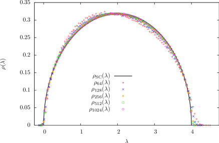
Figure 1: Density of eigenvalues $\rho_{N}(\lambda)$ of the matrix $\beta\chi^{-1}$ for $N=64,128,256,512,1024$ (in red, blue, yellow, green, violet respectively), $\beta J=1$ and $S=16\times 10^{3}$, and Wigner semicircular law $\rho_{\textrm{SC}}(\lambda)=1/(2\pi)\sqrt{4-(2-\lambda)^{2}}$ (black) as a function of $\lambda$. $\rho_{N}(\lambda)$ approaches $\rho_{\textrm{SC}}(\lambda)$ as $N$ is increased.

The finite-size fluctuations of $\lambda$ around $0$ are then investigated in Fig. 2. Defining $\phi$ in terms of $\lambda$ by Eq. (12), in Fig. 2 we depict the distribution $p_{N}(\phi)$ of the variable $\phi$ for several sizes $N$, and show that for increasing $N$, $p_{N}(\phi)$ approaches the TW distribution $p_{\textrm{GOE}}(\phi)$. Let us introduce the central moments

$$\mu^{N}_{1} \equiv \mathbb{E}_{N}[\phi],$$

$$\mu^{N}_{i} \equiv \mathbb{E}_{N}[(\phi-\mathbb{E}_{N}[\phi])^{i}]\,\forall i>1$$

of $p_{N}(\phi)$, and the central moments

$$\mu^{\textrm{GOE}}_{1} \equiv \mathbb{E}_{\textrm{GOE}}[\phi],$$

$$\mu^{\textrm{GOE}}_{i} \equiv \mathbb{E}_{\textrm{GOE}}[(\phi-\mathbb{E}_{\textrm{GOE}}[\phi])^{i}]\,\forall i>1$$

of the TW distribution, where

$$\mathbb{E}_{N}[\cdot] \equiv \int d\phi\,p_{N}(\phi)\cdot,$$

$$\mathbb{E}_{\textrm{GOE}}[\cdot] \equiv \int d\phi\,p_{{\textrm{GOE}}}(\phi)\cdot.$$

In the inset of Fig. 2 we depict $\mu^{N}_{i}$ for several sizes $N$ and $\mu_{i}^{\textrm{GOE}}$ as a function of $i$, showing that $\mu^{N}_{i}$ converges to $\mu^{\textrm{GOE}}_{i}$ as $N$ is increased.

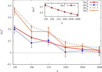
Figure 3: Relative difference $\Delta\mu^{N}_{i}$ between the central moments $\mu^{N}_{i}$ of the distribution $p_{N}(\phi)$ for $10^{5}\leq S\leq 4\times 10^{5}$, and the central moments $\mu^{\textrm{GOE}}_{i}$ of the Tracy-Widom distribution as a function of $N=128,256,512,1024,2048,4096$, for $i=2,3,4,5$ (in red, blue, black, orange respectively). For increasing $N$, $\mu^{N}_{i}$ approaches $\mu^{\textrm{GOE}}_{i}$, confirming the asymptotic independence of $z_{2}^{i}$ by each of the off-diagonal elements $x_{ij}$ for large $N$. Inset: relative difference of the first central moment $\Delta\mu^{N}_{1}$ as a function of $N$ (brown). $\Delta\mu^{N}_{1}$ approaches $0$ very slowly as $N$ is increased.

In Figure 3 this convergence is clarified by depicting $\Delta\mu^{N}_{i}\equiv(\mu^{N}_{i}-\mu_{i}^{\textrm{GOE}})/\mu_{i}^{\textrm{GOE}}$ for several values of $i>1$ as a function of $N$. $\Delta\mu^{N}_{i}$ is found to converge to $0$ for large $N$. In the inset of Fig. 3 we depict $\Delta\mu^{N}_{1}$ as a function of $N$, showing that the convergence of the first central moment with $N$ is much slower than that of the other central moments. It is interesting to observe that a slowly-converging first moment has been recently found also in experimentaltakeuchi2010universal and numericalrambeau data of models of growing interfaces where the TW distribution appears.

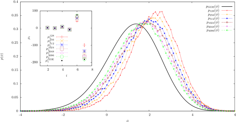
Figure 2: Distribution $p_{N}(\phi)$ for $N=128,256,512,1024,2048,4096$ (in red, yellow, blue, brown, violet, green respectively) and $10^{5}\leq S\leq 4\times 10^{5}$ samples, and the Tracy-Widom distribution $p_{\textrm{GOE}}(\phi)$ for the GOE ensemble (black), as a function of $\phi$. For increasing $N$, $p_{N}(\phi)$ approaches $p_{\textrm{GOE}}(\phi)$, confirming the asymptotic independence of the diagonal elements (11) by each of the off-diagonal elements $x_{ij}$ for large $N$. Inset: $\mu^{N}_{i}$ for sizes $N=128,256,512,1024,2048,4096$ (in red, yellow, blue, brown, violet, green respectively), $10^{5}\leq S\leq 4\times 10^{5}$, and $\mu_{i}^{\textrm{GOE}}$ (black) as a function of $i>1$.

The analytical argument proving the independence property of $z_{2}^{i}$ has been thus confirmed by this numerical calculation. Hence, the main result of this Section is that the finite-size fluctuations of the minimal eigenvalue of the susceptibility matrix $\beta\chi^{-1}$ in the TAP approximation for $\beta J=1$ are of order $N^{-2/3}$ and are distributed according to the TW law. These fluctuations have already been found to be of order $N^{-2/3}$ in a previous workbray1979evidence , and more recently reconsideredaspelmeier2008finite , following an independent derivation based on scaling arguments, even though the distribution has not been worked out. Our approach sheds some light on the nature of the scaling $N^{-2/3}$, which is non-trivial, since it comes from the $N^{-1/6}$-scaling of the TW distribution, which is found to govern the fluctuations of $\lambda$. Moreover, the fact that we find the same scaling as those found in such previous works can be considered as a consistency test of our calculation.

We now recall that both the derivation of this Section and the previously-developed analysis of Bray and Moorebray1979evidence rely on the TAP approximation, i. e. neglect the terms of the Plefka expansion (13) of order larger than $2$ in $\alpha$. As we will show in the following Section, these terms give a non-negligible contribution to the finite-size corrections of the TAP equations, and so to the finite-size fluctuations of the critical temperature, and thus must be definitely taken into account in a complete treatment.

IV Finite-size analysis of the susceptibility within the full Plefka expansion

In this Section we compute the inverse susceptibility matrix $\beta\chi^{-1}$ by taking into account all the terms of the Plefka expansion, in the effort to go beyond the TAP approximation of Section III. Notwithstanding its apparent difficulty, here we show that this task can be pursued by a direct inspection of the terms of the expansion. Indeed, let us formally write the free-energy $f$ a a seriesplefka1982convergence in $\alpha$,

$$f(\{m\},\beta)=\sum_{n=0}^{\infty}\alpha^{n}f_{n}(\{m\},\beta).$$ (13)

For $n<3$, the $f_{n}$s are given by Eq. (II). For $n>3$, $f_{n}$ is given by the sum of several different addendsyedidia2001idiosyncratic , which proliferate for increasing $n$. It is easy to show that at leading order in $N$, there is just one term contributing to $f_{n}$, and that such term can be written explicitly as

$$f_{n}(\{m\},\beta) \overset{N\rightarrow\infty}{\approx} \sum_{i_{1}>\cdots>i_{n-1}}x_{i_{1}i_{2}}x_{i_{2}i_{3}}\cdots x_{i_{n-1}i_{1}}$$

$$\times(1-m_{i_{1}}^{2})\times\cdots\times(1-m_{i_{n-1}}^{2}).$$

It follows that by plugging Eq. (IV) in Eq. (13) and computing $\beta\chi^{-1}$ for $m_{i}=0$, one obtains a simple expression for the inverse susceptibility at the paramagnetic solution

$$\beta\chi^{-1}_{ij} = -\alpha x_{ij}+\delta_{ij}\left(1+\alpha^{2}\sum_{k\neq i}x^{2}_{ki}+2\sum_{n=3}^{\infty}\alpha^{n}\sum_{i_{1}>\cdots>i_{n-1}}x_{ii_{1}}x_{i_{1}i_{2}}\cdots x_{i_{n-1}i}\right)$$ (15)

$$= -\alpha x_{ij}+\delta_{ij}\left(1+\beta^{2}J^{2}\right)+\delta_{ij}\frac{1}{\sqrt{N}}\left[(\beta J)^{2}z_{2}^{i}+2\sum_{n=3}^{\infty}\frac{(\beta J)^{n}}{\sqrt{(n-1)!}}z^{i}_{n}\right].$$

where

$$z^{i}_{n} \equiv \frac{\sqrt{(n-1)!}}{N^{\frac{n-1}{2}}}\times$$ (16)

$$\times\sum_{i_{1}>\cdots>i_{n-1}}x_{ii_{1}}x_{i_{1}i_{2}}\cdots x_{i_{n-1}i},\,\forall n>2.$$

According to Eq. (16), one has that at leading order in $N$

$$\mathbb{E}_{x}[z^{i}_{n}] = 0\,\forall n>2,$$

$$\mathbb{E}_{x}[(z^{i}_{n})^{2}] = 1\,\forall n>2,$$ (17)

where in the second line of Eq. (IV) the multiple sum defining $z_{n}^{i}$ has been evaluated at leading order in $N$.

We observe that the random variables $z^{i}_{n}$ and $x_{jk}$ in Eq. (15) are not independent, since each $z^{i}_{n}$ depends on the bond variables $\{x\}$. Following an argument similar to that given in Section III for $z_{2}^{i}$, we observe that, by Eq. (16) and at leading order in $N$, $z^{i}_{n}$ is given by a sum of $O(N^{n-1})$ terms which are all of the same order of magnitude. Each term is given by the product of $n-1$ bond variables $x_{ii_{1}}x_{i_{1}i_{2}}\cdots x_{i_{n-1}i}$ forming a loop passing by site $i$. For any fixed $i,j,k$ and $n$, only $O(N^{n-2})$ terms amongst the $O(N^{n-1})$ terms of $z^{i}_{n}$ are entangled with the random bond variable $x_{jk}$. It follows that at leading order in $N$, $z_{n}^{i}$ can be considered as independent by $x_{jk}$. Since the sum in the second line of Eq. (15) has a $1/\sqrt{N}$ factor multiplying each of the $z_{n}^{i}$s, we can consider the $z_{n}^{i}$ at leading order in $N$. Hence, in Eq. (15) we can consider each of $z_{n}^{i}$s as independent on $x_{jk}$.

In Appendix B we show that at leading order in $N$ the distribution of $z^{i}_{n}$ is a Gaussian with zero mean and unit variance for every $i$ and $n>2$, while in Appendix C we show that at leading order in $N$ the variables $\{z_{n}^{i}\}_{n,i}$ are mutually independent. Both these predictions are confirmed by numerical tests, illustrated in Appendix B and C respectively.

Hence, at leading order in $N$ the term in square brackets in Eq. (15) is nothing but the sum of independent Gaussian variables, and is thus equal to a random variable $\sigma\times\zeta_{i}$, where $\zeta_{i}$ is Gaussian with zero mean and unit variance, and

$$\sigma^{2} = 2(\beta J)^{4}+4\sum_{n=3}^{\infty}\frac{(\beta J)^{2n}}{(n-1)!}$$

$$= 2(\beta J)^{2}\{2(e^{(\beta J)^{2}}-1)-(\beta J)^{2}\}$$

It follows that Eq. (15) becomes

$$\beta\chi_{ij}^{-1} = -\alpha x_{ij}+\delta_{ij}\left(1+\beta^{2}J^{2}+\frac{\sigma}{\sqrt{N}}\zeta_{i}\right)$$ (18)

$$= -\alpha x^{\prime}_{ij}+\delta_{ij}\left(1+\beta^{2}J^{2}\right),$$

where

$$x^{\prime}_{ij}\equiv x_{ij}-\delta_{ij}\frac{\sigma}{\beta J}\zeta_{i}.$$ (19)

Because of the additional diagonal term in Eq. (19), the matrix $x^{\prime}_{ij}$ does not belong to the GOE ensemble. Notwithstanding this fact, it has been shown by Soshnikovsoshnikov1999universality that the presence of the diagonal elements in Eq. (19) does not alter the universal distribution of the maximal eigenvalue of $x^{\prime}_{ij}$, which is still distributed according to the TW law. Hence, denoting by $\lambda$ the minimal eigenvalue of $\beta\chi^{-1}$, we have

$$\lambda=(1-\beta J)^{2}+\frac{\beta J}{N^{2/3}}\phi_{\textrm{GOE}},$$ (20)

where $\phi_{\textrm{GOE}}$ is a random variable depending on the sample $x_{ij}$, and distributed according to the TW law.

In this Section we have calculated the inverse susceptibility matrix $\beta\chi^{-1}$, by considering the full Plefka expansion. In this framework additional diagonal terms are generated that were not present in the TAP approximation. These additional terms can be handled via a resummation to all orders in the Plefka expansion. As a result, we obtain that the fluctuations of the minimal eigenvalue $\lambda$ of the susceptibility $\beta\chi^{-1}$ are still governed by the TW law, as in the TAP case treated in Section III.

V Finite size fluctuations of the critical temperature

We can now define a finite-size critical temperature, and investigate its finite-size fluctuations due to disorder.

In the previous Sections we have shown that for a large but finite size $N$, the minimal eigenvalue of the inverse susceptibility matrix, i. e. the Hessian matrix of $\beta f(\{m\},\beta)$ evaluated in the paramagnetic minimum $m_{i}=0$, is a function of the temperature and of a quantity $\phi_{\textrm{GOE}}$, which depends on the realization of the disorder $\{x\}$. Since the TW law, i. e. the distribution of $\phi_{\textrm{GOE}}$, has support for both positive and negative values of $\phi_{\textrm{GOE}}$, the subleading term in Eq. (20) can be positive or negative. Accordingly, for samples $\{x\}$ such that $\phi_{\textrm{GOE}}<0$, there exists a value of $\beta J\approx 1$ such that $\lambda(\beta J)=0$, in such a way that the spin-glass susceptibility in the paramagnetic minimum diverges. This fact is physically meaningless, since there cannot be divergences in physical quantities at finite size. This apparent contradiction can be easily understood by observing that if $\lambda(\beta J)=0$, the true physical susceptibility is no more the paramagnetic one, but must be evaluated in the low-lying non-paramagnetic minima of the free-energy, whose appearance is driven by the emergent instability of the paramagnetic minimum.

According to this discussion, in the following we will consider only samples $\{x\}$ such that $\phi_{\textrm{GOE}}>0$. For these samples, the spectrum of the Hessian matrix at the paramagnetic minimum has positive support for every temperature: the paramagnetic solution is always stable and the paramagnetic susceptibility matrix $\chi$ is physical and finite. We define a pseudo-inverse critical temperature $\beta_{c}J$ as the value of $\beta J$ such that $\lambda$ has a minimum at $\beta_{c}J$

$$\left.\frac{d\lambda}{d\beta J}\right|_{\beta J=\beta_{c}J} \equiv 0$$ (21)

$$= -2(1-\beta_{c}J)+\frac{1}{N^{2/3}}\phi_{\textrm{GOE}}$$

where in the second line of Eq. (21), Eq. (20) has been used. This definition of pseudo-critical temperature has a clear physical interpretation: the stability of the paramagnetic minimum, which is encoded into the spectrum of the Hessian matrix $\beta\chi^{-1}$, has a minimum at $\beta=\beta_{c}$. According to Eq. (21), the finite-size critical temperature $\beta_{c}$ is given by

$$\beta_{c}J=1-\frac{1/2}{N^{2/3}}\phi_{\textrm{GOE}},$$ (22)

where $\phi_{\textrm{GOE}}$ depends on the sample $\{x\}$, and is distributed according to the TW law.

Eq. (22) shows that the pseudo-critical temperature of the SK model is a random variable depending on the realization of the quenched disorder: finite-size fluctuations of the pseudo-critical temperature are of order $N^{-2/3}$, and are distributed according to the TW law. This has to be considered the main result of this paper.

VI Discussion and conclusions

In this paper, the finite-size fluctuations of the critical temperature of the Sherrington-Kirkpatrick spin glass model have been investigated. The analysis is carried on within the framework of the Plefka expansion for the free-energy at fixed local magnetization. A direct investigation of the expansion shows that an infinite resummation of the series is required to describe the finite-size fluctuations of the critical temperature. By observing that the terms in the expansion can be treated as independent random variables, one can suitably define a finite-size critical temperature. Such a critical temperature has a unique value in the infinite-size limit, while exhibits fluctuations due to quenched disorder at finite sizes. These fluctuations with respect to the infinite-size value have been analyzed, and have been found to be of order $N^{-2/3}$, where $N$ is the system size, and to be distributed according to the Tracy-Widom distribution.
An analogous role of the TW distribution in the description of the critical properties of a physical system has also recently been clarified by Forrester et al.forrester2011non , showing that the TW law describes the finite-size corrections of the free-energy of a Yang-Mills theory in the neighborhood of its critical point.

The exponent $2/3$ describing the fluctuations of the pseudo-critical temperature stems from the fact that the finite-size fluctuations of the minimal eigenvalue $\lambda$ of the inverse susceptibility matrix are of order $N^{-2/3}$. Such a scaling for $\lambda$ at the critical temperature had already been obtained in a previous workbray1979evidence , where it was derived by a completely independent method, by taking into account only the first three terms of the Plefka expansion. The present work shows that a more careful treatment, including an infinite resummation of the expansion, is needed to handle finite-size effects. The exponent $2/3$ derived by Bray and Moorebray1979evidence is here rederived by establishing a connection with recently-developed results in random matrix theory, showing that the scaling $N^{-2/3}$ comes from the scaling of the Tracy-Widom distribution, which was still unknown when the paper by Bray and Moorebray1979evidence had been written.

As a possible development of the present work, it would be interesting to study the fluctuations of the critical temperature for a SK model where the couplings are distributed according to a power-law. Indeed, in a recent workbiroli2007top the distribution of the largest eigenvalue $\lambda$ of a random matrix $M$ whose entries $M_{ij}$ are power-law distributed as $p(M_{ij})\sim M_{ij}^{-1-\mu}$ has been studied. The authors show that if $\mu>4$ the fluctuations of $\lambda$ are of order $N^{-2/3}$ and are given by the TW distribution, while if $\mu<4$ the fluctuations are of order $N^{-2/\mu-1/2}$ and are governed by Fréchet’s statistics. This result could be directly applied to a SK model with power-law distributed couplings. In particular, it would be interesting to see if there exists a threshold in the exponent $\mu$ separating two different regimes of the fluctuations of $T_{c}$.

Another interesting perspective would be to generalize the present approach to realistic spin glass models with finite-range interactions. For instance, a huge amount of results has been quite recently obtained for the three-dimensional Ising spin glass banos2010nature ; hasenbusch2008critical ; alvarez2010static ; belletti2009depth ; contucci2007ultrametricity ; contucci2009structure ; krzakala2000spin ; PhysRevB.58.14852 , and for the short-range $p$-spin glass model in three dimensionsPhysRevB.58.12081 , yielding evidence for a finite-temperature phase transition. It would be interesting to try to generalize the present work to that systems, and compare the resulting fluctuations of the critical temperature with sample-to-sample fluctuations observed in these numerical works. Accordingly, the finite-size fluctuations deriving from the generalization of this work to the three-dimensional Ising spin glass could be hopefully compared with those observed in experimental spin glassesgunnarson1991static , such as $\textrm{Fe}_{0.5}\textrm{Mn}_{0.5}\textrm{TiO}_{3}$.

Finally, a recent numerical analysis billoire2011finite inspired by the present work has investigated the sample-to-sample fluctuations of a given pseudo-critical temperature for the SK model, which is different from that defined in this work. Even though the relatively small number of samples did not allow for a precise determination of the probability distribution of that pseudo-critical point, the analysis yields a scaling exponent equal to $1/3$, which is different from that of the pseudo-critical temperature defined here. As a consequence, the general scaling features of the pseudo-critical temperature seem to depend on the actual definition of the pseudo-critical point itself, even though different definitions of the pseudo-critical temperature must all converge to the infinite-size pseudo-critical temperature as the system size tends to infinity. As a future perspective, it would be interesting to investigate which amongst the features of the pseudo-critical point are definition-independent, if any.

Appendix A Proof of the asymptotic independence of $x_{ij}$ and $z_{2}^{i}$

Here we show that at leading order in $N$ the variables $x_{ij}$ and $z_{2}^{i}$ are independent, i. e. that at leading order in $N$

$$p_{N}(x_{ij}=x,z_{2}^{i}=z)=p_{N}(x_{ij}=x)\times p_{N}(z_{2}^{i}=z).$$ (23)

Let us explicitly write the left-hand size of Eq. (23) as

$$p_{N}(x_{ij}=x,z_{2}^{i}=z) = \mathbb{E}_{\{x_{ik}\}_{k\neq i}}[\delta(x_{ij}-x)\delta(z_{2}^{i}-z)],$$ (24)

$$= \mathbb{E}_{x_{ij}}\left[\delta(x_{ij}-x)\mathbb{E}_{\{x_{ik}\}_{k\neq i,k\neq j}}\left[\delta\left(\sqrt{N}\left(\frac{1}{N}\sum_{k\neq i,k\neq j}x_{ki}^{2}-1\right)-\overline{z}^{ij}_{2}\right)\right]\right]$$

Figure 4: Probability distribution $p_{N}(z_{4}^{1}=z)$ for $S=10^{5}$ and different values of $N=64,128,256,512,1024$ (in red, blue, yellow, green, violet respectively) together with a Gaussian distribution $1/\sqrt{2\pi}\textrm{e}^{-z^{2}/2}$ with zero mean and unit variance (black), as a function of $z$. As $N$ is increased $p_{N}(z_{4}^{1}=z)$ converges to $1/\sqrt{2\pi}\textrm{e}^{-z^{2}/2}$, as predicted by the analytical calculation, Eq. (31). Inset: zoom of the above plot explicitly showing the convergence of $p_{N}(z_{4}^{1}=z)$ to $1/\sqrt{2\pi}\textrm{e}^{-z^{2}/2}$ as $N$ is increased.

where $\mathbb{E}_{x_{lm},x_{no},\cdots}$ denotes the expectation value with respect to the probability distributions of the variables $x_{lm},x_{no},\cdots$, $\delta$ denotes the Dirac delta function, and

$$\overline{z}^{ij}_{2}\equiv z-\frac{x_{ij}^{2}}{\sqrt{N}}.$$ (25)

Proceeding systematically at leading order in $N$, the second expectation value in the second line of Eq. (24) is nothing but the probability that the variable $\sqrt{N}(\frac{1}{N}\sum_{k\neq i,k\neq j}x_{ki}^{2}-1)$ is equal to $\overline{z}^{ij}_{2}$. We observe that according to the central limit theorem, at leading order in $N$ this probability is given by

$$\mathbb{E}_{\{x_{ik}\}_{k\neq i,k\neq j}}\left[\delta\left(\sqrt{N}\left(\frac{1}{N}\sum_{k\neq i,k\neq j}x_{ki}^{2}-1\right)-\overline{z}^{ij}_{2}\right)\right]=$$

$$\frac{1}{\sqrt{4\pi}}\textrm{e}^{-\frac{\left(\overline{z}_{2}^{ij}\right)^{2}}{4}}.$$ (26)

By plugging Eq. (A) into Eq. (24) and using Eq. (25), one has

$$p_{N}(x_{ij}=x,z_{2}^{i}=z) = \frac{1}{\sqrt{4\pi}}\int dx_{ij}P(x_{ij})\delta(x_{ij}-x)\times$$ (27)

$$\times\textrm{e}^{-\frac{\left(z-x^{2}_{ij}/\sqrt{N}\right)^{2}}{4}}$$

$$= P(x)\frac{1}{\sqrt{4\pi}}\textrm{e}^{-\frac{\left(z-x^{2}/\sqrt{N}\right)^{2}}{4}}$$

$$= p_{N}(x_{ij}=x)\times p_{N}(z_{2}^{i}=z),$$

where in the first line Eq. (27) we explicitly wrote the expectation value with respect to $x_{ij}$ in terms of the probability distribution (2), while in the third line proceeded at leading order in $N$, and used Eq. (9).

Figure 5: $p_{1024}(z_{3}^{1}=z,z_{4}^{1}=z^{\prime})$ for $S=10^{5}$ samples (red), and the $N\rightarrow\infty$-limit of the right-hand side of Eq. (34) (black), as a function of $z,z^{\prime}$. For large $N$, $p_{N}(z_{3}^{1}=z,z_{4}^{1}=z^{\prime})$ equals $p_{N}(z_{3}^{1}=z)\times p_{N}(z_{4}^{1}=z^{\prime})$, as predicted by Eq. (34). Hence, at leading order in $N$ the variables $z_{3}^{1}$ and $z_{4}^{1}$ are independent.

Appendix B Computation of the probability distribution of $z_{n}^{i}$

Here we compute the probability distribution of $z_{n}^{i}$ at leading order in $N$ . Let us define a super index $L\equiv\{i_{1},\ldots,i_{n-1}\}$, where $L$ stands for ‘loop’, since $L$ represents a loop passing by the site $i$. Let us also set $X_{L}\equiv x_{ii_{1}}x_{i_{1}i_{2}}\cdots x_{i_{n-1}i}$. By Eq. (16) one has

$$z^{i}_{n} = \frac{\sqrt{(n-1)!}}{N^{\frac{n-1}{2}}}\sum_{L}X_{L},\forall n>2.$$ (28)

We observe that the probability distribution of $X_{L}$ is the same for every $L$. Hence, according to Eq. (28), $z_{n}^{i}$ is given by the sum of equally distributed random variables. Now pick two of these variables, $X_{L},X_{L^{\prime}}$. For some choices of $L,L^{\prime}$, $X_{L}$ and $X_{L^{\prime}}$ are not independent, since they can depend on the same bond variables $x_{ij}$. If one picks one variable $X_{L}$, the number of variables appearing in the sum (28) which are dependent on $X_{L}$ are those having at least one common edge with the edges of $X_{L}$. The number of these variables, at leading order in $N$, is $O(N^{n-2})$, since they are obtained by fixing one of the $n-1$ indexes $i_{1},\cdots,i_{n-1}$. The latter statement is equivalent to saying that if one picks at random two variables $X_{L},X_{L^{\prime}}$, the probability that they are correlated is

$$O(N^{n-2}/N^{n-1})=O(N^{-1}).$$ (29)

Hence, at leading order in $N$ we can treat the ensemble of the variables $\{X_{L}\}_{L}$ as independent. According to the central limit theorem, at leading order in $N$ the variable

$$\frac{\sqrt{(n-1)!}}{N^{\frac{n-1}{2}}}z^{i}_{n}=\frac{1}{\frac{N^{n-1}}{(n-1)!}}\sum_{L}X_{L}$$

is distributed according to a Gaussian distribution with mean $\mathbb{E}_{x}[X_{L}]=0$ and variance

$$\mathbb{E}_{x}\left[\left(\frac{\sqrt{(n-1)!}}{N^{\frac{n-1}{2}}}z^{i}_{n}\right)^{2}\right]=\frac{\mathbb{E}_{x}[X_{L}^{2}]}{\frac{N^{n-1}}{(n-1)!}}=\frac{1}{\frac{N^{n-1}}{(n-1)!}},$$ (30)

where in Eq. (30) Eq. (2) has been used. It follows that at leading order in $N$, $z_{n}^{i}$ is distributed according to a Gaussian distribution with zero mean and unit variance

$$p_{N}(z_{n}^{i}=z)\overset{N\rightarrow\infty}{\rightarrow}\frac{1}{\sqrt{2\pi}}\textrm{e}^{-\frac{z^{2}}{2}},$$ (31)

where $p_{N}(z_{n}^{i}=z)$ is defined as the probability that $z_{n}^{i}$ is equal to $z$ at size $N$.

Eq. (31) has been tested numerically for the first few values of $n$: $p_{N}(z_{n}^{i}=z)$ has been computed by generating $S\gg 1$ samples of $\{x\}$, and so of $z_{n}^{i}$. For $n=3,4$, the resulting probability distribution $p_{N}(z_{n}^{i}=z)$ converges to a Gaussian distribution with zero mean and unit variance as $N$ is increased, confirming the result (31). This convergence is shown in Fig. 4, where $p_{N}(z_{4}^{1}=z)$ is depicted for different values of $N$ together with the right-hand side of Eq. (31), as a function of $z$.

Appendix C Independence of the $z_{n}^{i}$s at leading order in $N$

Let us consider two distinct variables $z_{n}^{i},z_{m}^{j}$, and proceed at leading order in $N$.

Following the notation of Appendix B, we write Eq. (16) as

$$z^{i}_{n} = \frac{\sqrt{(n-1)!}}{N^{\frac{n-1}{2}}}\sum_{L}X_{L},$$ (32)

$$z^{j}_{m} = \frac{\sqrt{(m-1)!}}{N^{\frac{m-1}{2}}}\sum_{L^{\prime}}X_{L^{\prime}},$$ (33)

where $L,L^{\prime}$ represent a loop of length $n,m$ passing by the site $i,j$ respectively. Some of the variables $X_{L}$ depend on some of the variables $X_{L^{\prime}}$, because they can depend on the same bond variables $x_{ij}$. Let us pick at random one variable $X_{L}$ appearing in $z_{n}^{i}$, and count the number of variables $X_{L^{\prime}}$ in $z_{m}^{j}$ that are dependent on $X_{L}$. At leading order in $N$, these are given by the number of $X_{L^{\prime}}$ having at least one common bond with $X_{L}$, and are $O(N^{m-2})$. Hence, if one picks at random two variables $X_{L},X_{L^{\prime}}$ in Eqs. (32), (33) respectively, the probability that $X_{L},X_{L^{\prime}}$ are dependent is

$$O(N^{m-2}/N^{m-1})=O(N^{-1}).$$

It follows that $z_{n}^{i}$ and $z_{m}^{j}$ are independent at leading order in $N$, i. e. for $N\rightarrow\infty$

$$p_{N}(z_{n}^{i}=z,z_{m}^{j}=z^{\prime})=p_{N}(z_{n}^{i}=z)\times p_{N}(z_{m}^{j}=z^{\prime}),$$ (34)

where $p_{N}(z_{n}^{i}=z,z_{m}^{j}=z^{\prime})$ denotes the joint probability that $z_{n}^{i}$ equals $z$ and $z_{m}^{j}$ equals $z^{\prime}$, at fixed size $N$.

Eq. (34) has been tested numerically for $n=3,m=4$: $p_{N}(z_{3}^{1}=z,z_{4}^{1}=z^{\prime})$ has been computed by generating a number $S\gg 1$ of samples of $\{x\}$, and so of $z_{3}^{1},z_{4}^{1}$. As a result, the left-hand side of Eq. (34) converges to the right-hand side as $N$ is increased, confirming the predictions of the above analytical argument. This is shown in Fig. 5, where $p_{1024}(z_{3}^{1}=z,z_{4}^{1}=z^{\prime})$ is depicted together with the $N\rightarrow\infty$-limit of the right-hand side of Eq. (34) (see Eq. (31)), as a function of $z,z^{\prime}$.

References

- [1] T. D. Lee and C. N. Yang. Statistical theory of equations of state and phase transitions. II. Lattice gas and Ising model. Physical Review, 87(3):410–419, 1952.
- [2] C. Yang. Statistical theory of equations of state and phase transitions. I. Theory of condensation. Physical Review, 87(3):404–409, 1952.
- [3] K. Huang. Statistical mechanics. Wiley, 1987.
- [4] M. Biskup, C. Borgs, J. T. Chayes, L. J. Kleinwaks, and R. Koteckỳ. General theory of Lee-Yang zeros in models with first-order phase transitions. Physical Review Letters, 84(21):4794–4797, 2000.
- [5] D. Ruelle. Extension of the Lee-Yang circle theorem. Physical Review Letters, 26(6):303–304, 1971.
- [6] C. Monthus and T. Garel. Delocalization transition of the selective interface model: distribution of pseudo-critical temperatures. Journal of Statistical Mechanics: Theory and Experiment, 2005(12):P12011, 2005.
- [7] C. Monthus and T. Garel. Distribution of pseudo-critical temperatures and lack of self-averaging in disordered Poland-Scheraga models with different loop exponents. The European Physical Journal B-Condensed Matter and Complex Systems, 48(3):393–403, 2005.
- [8] F. Iglói, Y. C. Lin, H. Rieger, and C. Monthus. Finite-size scaling of pseudocritical point distributions in the random transverse-field Ising chain. Physical Review B, 76(6):064421, 2007.
- [9] C. Monthus and T. Garel. Freezing transition of the directed polymer in a random medium: location of the critical temperature and unusual critical properties. Physical Review E, 74(1):011101, 2006.
- [10] T. Sarlat, A. Billoire, G. Biroli, and J. P. Bouchaud. Predictive power of MCT: numerical testing and finite size scaling for a mean field spin glass. Journal of Statistical Mechanics: Theory and Experiment, 2009(08):P08014, 2009.
- [11] E. J. Gumbel. Statistics of extremes. New York: Columbia University Press, 1958.
- [12] M. L. Mehta. Random matrices. Academic press, 2004.
- [13] Higher Ed. Press, editor. Distribution functions for largest eigenvalues and their applications, volume 1. C. A. Tracy and H. Widom in Proc. International Congress of Mathematicians (Beijing, 2002), 2002.
- [14] C. A. Tracy and H. Widom. On orthogonal and symplectic matrix ensembles. Communications in Mathematical Physics, 177(3):727–754, 1996.
- [15] C. A. Tracy and H. Widom. Level-spacing distributions and the Airy kernel. Communications in Mathematical Physics, 159(1):151–174, 1994.
- [16] C. A. Tracy and H. Widom. Level-spacing distributions and the Airy kernel. Physics Letters B, 305(1-2):115–118, 1993.
- [17] K. Johansson. Shape fluctuations and random matrices. Communications in Mathematical Physics, 209(2):437–476, 2000.
- [18] J. Baik and E. M. Rains. Limiting distributions for a polynuclear growth model with external sources. Journal of Statistical Physics, 100(3):523–541, 2000.
- [19] M. Prähofer and H. Spohn. Universal distributions for growth processes in dimensions and random matrices. Physical Review Letters, 84(21):4882–4885, 2000.
- [20] G. Biroli, J. P. Bouchaud, and M. Potters. Extreme value problems in random matrix theory and other disordered systems. Journal of Statistical Mechanics: Theory and Experiment, 2007(07):P07019, 2007.
- [21] D. Sherrington and S. Kirkpatrick. Solvable model of a spin-glass. Physical Review Letters, 35(26):1792–1796, 1975.
- [22] G. Parisi. The order parameter for spin glasses: A function on the interval 0-1. Journal of Physics A: Mathematical and General, 13:1101, 1980.
- [23] G. Parisi. Order parameter for spin-glasses. Physical Review Letters, 50(24):1946–1948, Jun 1983.
- [24] M. Talagrand. The generalized Parisi formula. Comptes Rendus Mathematique, 337(2):111–114, 2003.
- [25] M. Mézard, G. Parisi, and M. A. Virasoro. Spin glass theory and beyond. World Scientific, 1987.
- [26] M. Mézard and A. Montanari. Information, physics and computation. Oxford University Press, 2009.
- [27] H. Nishimori. Statistical Physics of Spin Glasses and Information Processing: An Introduction. Oxford University Press, Oxford, UK, 2001.
- [28] D. J. Thouless, P. W. Anderson, and R. G. Palmer. Solution of ‘Solvable model of a spin glass’. Philosophical Magazine, 35(3):593–601, 1977.
- [29] T. Plefka. Convergence condition of the TAP equation for the infinite-ranged Ising spin glass model. Journal of Physics A: Mathematical and general, 15:1971, 1982.
- [30] A. Georges, M. Mézard, and J. S. Yedidia. Low-temperature phase of the Ising spin glass on a hypercubic lattice. Physical Review Letters, 64(24):2937–2940, 1990.
- [31] J. S. Yedidia and A. Georges. The fully frustrated Ising model in infinite dimensions. Journal of physics. A: Mathematical and General, 23(11):2165–2171, 1990.
- [32] T. Yokota. Ordered phase for the infinite-range Potts-glass model. Physical Review B, 51(2):962–971, 1995.
- [33] T. Plefka. Expansion of the Gibbs potential for quantum many-body systems: General formalism with applications to the spin glass and the weakly nonideal Bose gas. Physical Review E, 73(1):016129, 2006.
- [34] H. Ishii and T. Yamamoto. Effect of a transverse field on the spin glass freezing in the Sherrington-Kirkpatrick model. Journal of physics. C: Solid State Physics, 18(33):6225–6237, 1985.
- [35] L. De Cesare, K. L. Walasek, and K. Walasek. Cavity-field approach to quantum spin glasses: The Ising spin glass in a transverse field. Physical Review B, 45(14):8127, 1992.
- [36] G. Biroli and L. F. Cugliandolo. Quantum Thouless-Anderson-Palmer equations for glassy systems. Physical Review B, 64(1):014206, 2001.
- [37] J. S. Yedidia. An idiosyncratic journey beyond mean field theory. Advanced mean field methods: Theory and practice, pages 21–36, 2001.
- [38] E. P. Wigner. Characteristic vectors of bordered matrices with infinite dimensions. The Annals of Mathematics, 62(3):548–564, 1955.
- [39] Y. V. Fyodorov. Introduction to the random matrix theory: Gaussian unitary ensemble and beyond, in Recent perspectives in random matrix theory and number theory, volume 322, page 31. Cambridge Univ. Pr., 2005.
- [40] G. Parisi and T. Rizzo. Large deviations in the free energy of mean-field spin glasses. Physical Review Letters, 101(11):117205, 2008.
- [41] G. Parisi and T. Rizzo. Phase diagram and large deviations in the free energy of mean-field spin glasses. Physical Review B, 79(13):134205, 2009.
- [42] G. Parisi and T. Rizzo. Universality and deviations in disordered systems. Physical Review B, 81(9):094201, 2010.
- [43] J. Stäring, B. Mehlig, Y. V. Fyodorov, and J. M. Luck. Random symmetric matrices with a constraint: The spectral density of random impedance networks. Physical Review E, 67(4):047101, 2003.
- [44] P. Shukla. Random matrices with correlated elements: A model for disorder with interactions. Physical Review E, 71(2):026226, 2005.
- [45] Z. Bai and W. Zhou. Large sample covariance matrices without independence structures in columns. Statistica Sinica, 18(2):425, 2008.
- [46] K. A. Takeuchi and M. Sano. Universal fluctuations of growing interfaces: evidence in turbulent liquid crystals. Physical Review Letters, 104(23):230601, 2010.
- [47] J. Rambeau and G. Schehr. To be published.
- [48] A. J. Bray and M. A. Moore. Evidence for massless modes in the ‘solvable model’ of a spin glass. Journal of Physics C: Solid State Physics, 12:L441, 1979.
- [49] T. Aspelmeier, A. Billoire, E. Marinari, and M. A. Moore. Finite-size corrections in the Sherrington-Kirkpatrick model. Journal of Physics A: Mathematical and Theoretical, 41(32):324008 (21pp)–, 2008.
- [50] A. Soshnikov. Universality at the edge of the spectrum in Wigner random matrices. Communications in mathematical physics, 207(3):697–733, 1999.
- [51] P. J. Forrester, S. N. Majumdar, and G. Schehr. Non-intersecting Brownian walkers and Yang-Mills theory on the sphere. Nuclear Physics B, 844:500–526, 2011.
- [52] G. Biroli, J. P. Bouchaud, and M. Potters. On the top eigenvalue of heavy-tailed random matrices. Europhysics Letters, 78:10001, 2007.
- [53] R. A. Banos, A. Cruz, L. A. Fernandez, J. M. Gil-Narvion, A. Gordillo-Guerrero, M. Guidetti, A. Maiorano, F. Mantovani, E. Marinari, V. Martin-Mayor, et al. Nature of the spin-glass phase at experimental length scales. Journal of Statistical Mechanics: Theory and Experiment, 2010(06):P06026, 2010.
- [54] M. Hasenbusch, A. Pelissetto, and E. Vicari. Critical behavior of three-dimensional Ising spin glass models. Physical Review B, 78(21):214205, 2008.
- [55] R. Alvarez Baños, A. Cruz, L. A. Fernandez, J. M. Gil-Narvion, A. Gordillo-Guerrero, M. Guidetti, A. Maiorano, F. Mantovani, E. Marinari, V. Martin-Mayor, et al. Static versus dynamic heterogeneities in the Edwards-Anderson Ising spin glass. Physical Review Letters, 105(17):177202, 2010.
- [56] F. Belletti, A. Cruz, L. A. Fernandez, A. Gordillo-Guerrero, M. Guidetti, A. Maiorano, F. Mantovani, E. Marinari, V. Martin-Mayor, J. Monforte, et al. An in-depth view of the microscopic dynamics of Ising spin glasses at fixed temperature. Journal of Statistical Physics, 135(5):1121–1158, 2009.
- [57] P. Contucci, C. Giardinà, C. Giberti, G. Parisi, and C. Vernia. Ultrametricity in the Edwards-Anderson model. Physical Review Letters, 99(5):057206, 2007.
- [58] P. Contucci, C. Giardinà, C. Giberti, G. Parisi, and C. Vernia. Structure of correlations in three dimensional spin glasses. Physical Review Letters, 103(1):017201, 2009.
- [59] F. Krzakala and O. C. Martin. Spin and link overlaps in three-dimensional spin glasses. Physical Review Letters, 85(14):3013–3016, 2000.
- [60] E. Marinari, G. Parisi, and J. J. Ruiz-Lorenzo. Phase structure of the three-dimensional Edwards-Anderson spin glass. Physical Review B, 58(22):14852–14863, 1998.
- [61] M. Campellone, B. Coluzzi, and G. Parisi. Numerical study of a short-range -spin glass model in three dimensions. Physical Review B, 58(18):12081–12089, 1998.
- [62] K. Gunnarsson, P. Svedlindh, P. Nordblad, L. Lundgren, H. Aruga, and A. Ito. Static scaling in a short-range Ising spin glass. Physical Review B, 43(10):8199–8203, 1991.
- [63] A. Billoire, L. A. Fernandez, A. Maiorano, E. Marinari, V. Martin-Mayor, and D. Yllanes. Finite-size scaling analysis of the distributions of pseudo-critical temperatures in spin glasses. Arxiv preprint arXiv:1108.1336, 2011.