Multiple-Source Single-Sink Maximum Flow in Directed Planar Graphs in $O(\textrm{diameter}\cdot n\log n)$ Time

Abstract

We develop a new technique for computing maximum flow in directed planar graphs with multiple sources and a single sink that significantly deviates from previously known techniques for flow problems. This gives rise to an $O(\textrm{diameter}\cdot n\log n)$ algorithm for the problem.

1 Introduction

The study of maximum flow in planar graphs has a long history. In 1956, Ford and Fulkerson introduced the max $st$-flow problem, gave a generic augmenting-path algorithm, and also gave a particular augmenting-path algorithm for the case of a planar graph where $s$ and $t$ are on the same face (that face is traditionally designated to be the infinite face). Researchers have since published many algorithmic results proving running-time bounds on max $st$-flow for (a) planar graphs where $s$ and $t$ are on the same face, (b) undirected planar graphs where $s$ and $t$ are arbitrary, and (c) directed planar graphs where $s$ and $t$ are arbitrary. The best bounds known are (a) $O(n)$ [5], (b) $O(n\log\log n)$ [6], and (c) $O(n\log n)$ [2], where $n$ is the number of nodes in the graph.

This paper is concerned with the maximum flow problem in the presence of multiple sources. In max-flow applied to general graphs, multiple sources presents no problem: one can reduce the problem to the single-source case by introducing an artificial source and connecting it to all the sources. However, as Miller and Naor [10] pointed out, this reduction violates planarity unless all the sources are on the same face to begin with. Miller and Naor raise the question of computing a maximum flow in a planar graph with multiple sources and multiple sinks. Until recently, the best known algorithm for computing multiple-source max-flow in a planar graph is to use the reduction in conjunction with a max-flow algorithm for general graphs. That is, no planarity-exploiting algorithm was known for the problem. A few months after developing the technique described in this paper we developed with collaborators an algorithm for the more general problem of maximum flow in planar graphs with multiple sources and sinks [3] which runs in $O(n\log^{3}n)$ time and uses a recursive approach. Given these recent developments, the algorithm presented here is mostly interesting for the new technique developed.

In this paper we present an alternative algorithm for the maximum flow problem with multiple sources and a single sink in planar graphs that runs in $O(\textrm{diameter}\cdot n\log n)$ time. The diameter of a graph is defined as the maximum over all pairs of nodes of the minimum number of edges in a path connecting the pair. Essentially, we start with a non-feasible flow that dominates a maximum flow, and convert it into a feasible maximum preflow by eliminating negative-length cycles in the dual graph. The main algorithmic tool is a modification of an algorithm of Klein [9] for finding multiple-source shortest paths in planar graphs with nonnegative lengths; our modification identifies and eliminates negative-length cycles. This approach is significantly different than all previously known maximum-flow algorithms. While the relation between flow in the primal graph and shortest paths in the dual graph has been used in many algorithms for planar flow, considering fundamentally non-feasible flows and handling negative cycles is novel. We believe that this is an interesting algorithmic technique and are hopeful it will be useful beyond the current context.

1.1 Applications

Schrijver [12] has written about the history of the maximum-flow problem. Ford and Fulkerson, who worked at RAND, were apparently motivated by a classified memo of Harris and Ross on interdiction of the Soviet railroad system. That memo, which was declassified, contains a diagram of a planar network that models the Soviet railroad system and has multiple sources and a single sink.

A more realistic motivation comes from selecting multiple nonoverlapping regions in a planar structure. Consider, for example, the following image-segmentation problem. A grid is given in which each vertex represents a pixel, and edges connect orthogonally adjacent pixels. Each edge is assigned a cost such that the edge between two similar pixels has higher cost than that between two very different pixels. In addition, each pixel is assigned a weight. High weight reflects a high likelihood that the pixel belongs to the foreground; a low-weight pixel is more likely to belong to the background.

The goal is to find a partition of the pixels into foreground and background to minimize the sum

weight of background pixels

$$+$$ cost of edges between foreground pixels and background pixels

subject to the constraints that, for each component $K$ of foreground pixels, the boundary of $K$ forms a closed curve in the planar dual that surrounds all of $K$ (essentially that the component is simply connected).

This problem can be reduced to multiple-source, single-sink max-flow in a planar graph (in fact, essentially the grid). For each pixel vertex $v$, a new vertex $v^{\prime}$, designated a source, is introduced and connected only to $v$. Then the sink is connected to the pixels at the outer boundary of the grid. See [4] for similar applications in computer vision.

1.2 Related Work

Most of the algorithms for computing maximum flow in general (i.e., non-planar) graphs build a maximum flow by starting from the zero flow and iteratively pushing flow without violating arc capacities. Traditional augmenting path algorithms, as well as more modern blocking flow algorithms, push flow from the source to the sink at each iteration, thus maintaining a feasible flow (i.e., a flow assignment that respects capacities and obeys conservation at non-terminals) at all times. Push-relabel algorithms relax the conservation requirement and maintain a feasible preflow rather than a feasible flow. However, none of these algorithms maintains a flow assignment that violates arc capacities.

There are algorithms for maximum flow in planar graphs that do use flow assignments that violate capacities [11, 10]. However, these violations are not fundamental in the sense that the flow does respect capacities up to a circulation (a flow with no sources or sinks). In other words, the flow may over-saturate some arcs, but no cut is over-saturated. We call such flows quasi-feasible flows.

The value of a flow that does over-saturate some cuts is higher than that of a maximum flow. This situation can be identified by detecting a negative-length cycle in the dual of the residual graph. One of the algorithms in [10] uses this property in a parametric search for the value of the maximum flow. When a quasi-feasible flow with maximum value is found, it is converted into a feasible one. This approach is not suitable for dealing with multiple sources because the size of the search space grows exponentially with the number of sources.

Our approach is the first to use and handle fundamentally infeasible flows. Instead of interpreting the existence of negative cycles as a witness that a given flow should not be used to obtain a maximum feasible flow, we use the negative cycles to direct us in transforming a fundamentally non-feasible flow into a maximum feasible flow. A negative-length cycle whose length is $-c$ corresponds to a cut that is over saturated by $c$ units of flow. This implies that the flow should be decreased by pushing $c$ units of flow back from the sink across that cut.

2 Preliminaries

In this section we provide basic definitions and notions that are useful in presenting the algorithm. Additional definitions and known facts that are relevant to the proof of correctness and to the analysis are presented later on.

We assume the reader is familiar with the basic definitions of planar embedded graphs and their duals (cf. [2]). Let $G=\langle V,A\rangle$ be a planar embedded graph with node-set $V$ and arc-set $A$. For notational simplicity, we assume here and henceforth that $G$ is connected and has no parallel edges and no self-loops. For each arc $a$ in the arc-set $A$, we define two oppositely directed darts, one in the same orientation as $a$ (which we sometimes identify with $a$) and one in the opposite orientation. We define $\mbox{rev}(\cdot)$ to be the function that takes each dart to the corresponding dart in the opposite direction. It is notationally convenient to equate the edges, arcs and darts of $G$ with the edges, arcs and darts of the dual $G^{*}$. It is well-known that contracting an edge that is not a self-loop corresponds to deleting it in the dual, and that a set of darts forms a simple directed cycle in $G$ iff it forms a simple directed cut in the dual $G^{*}$ [13]; see Fig. 1.

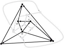
Figure 1: A primal graph (black) and its dual (gray). The cut $\vec{\delta}(\{u,v,w\})$ in the primal corresponds to a counterclockwise dual cycle (dashed arcs).

Given a length assignment $\mbox{length}(\cdot)$ on the darts, we extend it to sets $D$ of darts by $\mbox{length}(D)=\sum_{d\in D}\mbox{length}(d)$. For a set $X$ of nodes, let $\vec{\delta}(X)$ denote the set of darts crossing the cut $(X,V-X)$. Namely, $\vec{\delta}(X)=\{d:\text{tail}(d)\in X,\text{head}(d)\notin X\}$. Let $T$ be a rooted spanning tree of $G^{*}$. For a node $v\in G^{*}$, let $T[v]$ denote the unique root-to-$v$ path in $T$. The reduced length of $d$ with respect to $T$ is defined by

$$\mbox{length}_{T}(d)=\mbox{length}(d)+\mbox{length}(T[\text{tail}_{G^{*}}(d)])-\mbox{length}(T[\text{head}_{G^{*}}(d)])$$ (1)

The edges of $G$ not in $T$ form a spanning tree $\tau$ of $G$. A dart $d$ is unrelaxed if $\mbox{length}_{T}(d)<0$. Note that, by definition, only darts not in $T$ can be unrelaxed. A leafmost unrelaxed dart is an unrelaxed dart $d$ of $\tau$ such that no proper descendant of $d$ in $\tau$ is unrelaxed. For a dart $d$ not in $T$, the elementary cycle of $d$ with respect to $T$ in $G^{*}$ is the cycle composed of $d$ and the unique path in $T$ between the endpoints of $d$.

2.1 Flow

Let $S\subset V$ be a set vertices called sources, and let $t\notin S$ be vertex called sink.

A flow assignment $f(\cdot)$ in $G$ is a real-valued function on the darts of $G$ satisfying antisymmetry:

$$f(\mbox{rev}(d))=-f(d)$$

A capacity assignment $c(\cdot)$ is a real-valued function on darts. A flow assignment $f(\cdot)$ is feasible or respects capacities if, for every dart $d$, $f(d)\leq c(d)$. Note that, by antisymmetry, $f(d)\leq c(d)$ implies $f(\mbox{rev}(d))\geq-c(d)$. Thus a negative capacity on a dart acts as a lower bound on the flow on the reverse dart.

For a given flow assignment $f(\cdot)$, the net inflow (or just inflow) node $v$ is $\textrm{inflow}_{f}(v)=\sum_{d\in A:\text{head}(d)=v}f(d)$. The outflow of $v$ is $\textrm{outflow}_{f}(v)=-\textrm{inflow}_{f}(v)$. The value of $f(\cdot)$ is the inflow at the sink, $\textrm{inflow}_{f}(t)$. A flow assignment $f(\cdot)$ is said to obey conservation at node $v$ if $\textrm{inflow}_{f}(v)=0$. A flow assignment is a circulation if it obeys conservation at all nodes. A flow assignment is a flow if it obeys conservation at every node other than the sources and sink. It is a preflow if for every node other than the sources, $\textrm{inflow}_{f}(v)\geq 0$.

For two flow assignments $f,f^{\prime}$, the addition $f+f^{\prime}$ is the flow that assigns $f(d)+f^{\prime}(d)$ to every dart $d$. A flow assignment $f$ is a quasi-feasible flow if there exists a circulation $\phi$ such that $f+\phi$ is a feasible flow. This concept is not new, but it is so central to our algorithm that we introduce a name for it.

The residual graph of $G$ with respect to a flow assignment $f(\cdot)$ is the graph $G_{f}$ with the same arc-set, node-set and sink, and with capacity assignment $c_{f}(\cdot)$ defined as follows. For every dart $d$, $c_{f}(d)=c(d)-f(d)$.

Given a feasible preflow $f_{+}$ in a planar graph, there exists an $O(n\log n)$-time algorithm that converts $f_{+}$ into a feasible flow $f$ with the same value (cf. [7]). In fact, this can be done in linear time by first canceling flow cycles using the technique of Kaplan and Nussbaum [8], and then by sending any excess flow from back to the sources in topological sort order.

2.2 Quasi-Feasible Flows and Negative-Length Dual Cycles

Miller and Naor prove that $f$ is a quasi-feasible flow in $G$ if and only if $G^{*}_{f}$ contains no negative-length cycles. Intuitively, a negative-length cycle in the dual corresponds to a primal cut whose residual capacity is negative. That is, the corresponding cut is over-saturated. Since a circulation obeys conservation at all nodes it does not change the total flow across any cut. Therefore, there exists no circulation whose addition to $f$ would make it feasible. Conversely, they show that if $G_{f}^{*}$ has no negative-length cycles, then shortest path distances from any arbitrary node in the dual define a feasible circulation in the primal.

2.2.1 Potentials, Clockwise and Left-of

The set of circulations in a graph forms a vector space, called the cycle space of the graph. For each face $f$, let $\bm{u}_{f}$ be the vector that assigns flow value 1 to each dart in the clockwise boundary of the face. Each such vector is in the cycle space. Moreover, the set $\{\bm{u}_{f}\ :\ f\neq f_{\infty}\}$ is a basis for the cycle space. Therefore every circulation can be written as a linear combination $\sum_{f}p_{f}\bm{u}_{f}$. The coefficients $p_{f}$ are called face potentials. By convention, the potential of $f_{\infty}$ is zero.

A circulation is clockwise (counterclockwise) if the corresponding potentials are nonnegative (nonpositive). (A circulation can be neither.) For $u$-to-$v$ paths $P$ and $Q$, we say $P$ is left of (right of)$Q$ if $P\mbox{rev}(Q)$ is clockwise (counterclockwise).

2.2.2 Price Functions and Reduced lengths

For a directed graph $G$ with arc-lengths $\ell(\cdot)$, a price function is a function $\phi$ from the nodes of $G$ to the reals. For an arc $uv$, the reduced length with respect to $\phi$ is $\ell_{\phi}(uv)=\ell(uv)+\phi(u)-\phi(v)$. For any nodes $s$ and $t$, for any $s$-to-$t$ path $P$, $\ell_{\phi}(P)=\ell(P)+\phi(s)-\phi(t)$. This shows that an $s$-to-$t$ path is shortest with respect to $\ell_{\phi}(\cdot)$ iff it is shortest with respect to $\ell(\cdot)$. In particular, the reduced length of any cycle is the same as its length.

2.2.3 Winding Numbers

For a curve $\gamma$ in the plane and a path $P$, the winding number of $P$ about $\gamma$ is the number of times $P$ crosses $\gamma$ right-to-left, minus the number of times it crosses $\gamma$ left-to-right.

3 The Algorithm

We describe an algorithm that, given a graph $G$ with $n$ nodes, a sink $t$ incident to the infinite face $f_{\infty}$, and multiple sources, computes a maximum flow from the sources to $t$ in time $O(\textrm{diameter}\cdot n\log n)$, where diameter is the diameter of the face-vertex incidence graph of $G$. Initially, each dart $d$ has a non-negative capacity, which we denote by $\mbox{length}(d)$ since we will interpret it as a length in the dual. During the execution of the algorithm, the length assignment $\mbox{length}(\cdot)$ is modified. Even though the algorithm does not explicitly maintain a flow at all times, we will refer throughout the paper to the flow pushed by the algorithm. At any given point in the execution of the algorithm we can interpret the lengths of darts in the dual as their residual capacities in the primal. By the flow pushed by the algorithm, we mean the flow that would induce these residual capacities.

Algorithm 1 Multiple-source single-sink maximum flow $(G,S,t,c_{0})$

Input: planar directed graph $G$ with capacities $c_{0}$, source set $S$, sink $t$ incident to $f_{\infty}$
Output: a maximum feasible flow $f$

1:  $\mbox{length}(d):=c_{0}(d)$ for every dart $d$

2:  initialize spanning tree $T$ of ${G^{*}}$ rooted at $f_{\infty}$ using right-first-search

3:  let $\tau$ be the spanning tree of $G$ consisting of edges not in $T$, and root $\tau$ at $t$

4:  for each source $s\in S$ 

5:     for each dart $d$ on the $s$-to-$t$ path in $\tau$ 

6:        $\mbox{length}(d):=\mbox{length}(d)-\mbox{length}(\delta(\{s\}))$

7:        $\mbox{length}(\mbox{rev}(d)):=\mbox{length}(\mbox{rev}(d))+\mbox{length}(\delta(\{s\}))$

8:  while there exist unrelaxed darts in ${G^{*}}$ 

9:     let $\hat{d}$ be an unrelaxed dart that is leafmost in $\tau$

10:     if $\hat{d}$ is not a back-edge in $T$ then  //perform a pivot

11:        remove from $T$ the parent edge of $\text{head}_{G^{*}}(\hat{d})$ and insert $\hat{d}$ into $T$

12:     else  // fix a negative cycle by pushing back flow

13:        let $C$ denote the elementary cycle of $\hat{d}$ with respect to $T$ in $G^{*}$

14:        for each dart $d$ of the $\hat{d}$-to-$t$ path of darts in the primal spanning tree $\tau$

$$\mbox{length}(d):=\mbox{length}(d)+|\mbox{length}(C)|$$

$$\mbox{length}(\mbox{rev}(d)):=\mbox{length}(\mbox{rev}(d))-|\mbox{length}(C)|$$

15:        for every dart $d$ strictly enclosed by $C$ 

16:           $f(d):=c_{0}(d)-\mbox{length}_{T}(d)$

17:           in $G$, contract $d$ //in ${G^{*}}$, delete $d$

18:  $f(d):=c_{0}(d)-\mbox{length}_{T}(d)$ for every dart $d$

19:  convert the preflow $f$ into a flow.

The algorithm starts by pushing an infeasible flow that saturates $\delta(s)$ from every source $s$ to $t$ (Line 4). It then starts to reduce that flow in order to make it feasible. This is done by using a spanning tree $\tau$ of $G$ and a spanning tree $T$ of ${G^{*}}$ such that each edge is in exactly one of these trees. The algorithm repeatedly identifies a negative cycle $C$ in ${G^{*}}$, which corresponds in $G$ to an over-saturated cut. Line 14 decreases the lengths of darts on a primal path in $\tau$ that starts at the sink $t$ and ends at some node $v$ (a face in ${G^{*}}$) that is enclosed by $C$. We call such a path a pushback path. This change corresponds to pushing flow back from the sink to $v$ along the pushback path, making the over-saturated cut exactly saturated. We call the negative-turned-zero-length cycle $C$ a processed cycle. Processed cycles enclose no negative cycles. This implies that there exists a feasible preflow that saturates the cut corresponding to a processed cycle (see Lemma 5). The algorithm records that preflow (Line 16) and contracts the source-side of the cut into a single node referred to as a super-source.

When no negative length cycles are left in the contracted graph, the flow pushed by the algorithm is quasi-feasible. That is, the flow pushed by the algorithm is equivalent, up to a circulation, to a feasible flow in the contracted graph. Combining this feasible flow in the contracted graph and the preflows recorded at the times cycles were processed yields a maximum feasible preflow for the original uncontracted graph. In a final step, this feasible preflow is converted into a feasible flow.

We now describe in more detail how negative cycles are identified and processed by the algorithm. The algorithm maintains a spanning tree $T$ of ${G^{*}}$ rooted at the infinite face $f_{\infty}$ of $G$, and a spanning tree $\tau$ of $G$, rooted at the sink $t$. The tree $\tau$ consists of the edges not in $T$. The algorithm tries to transform $T$ into a shortest-path tree by pivoting into $T$ unrelaxed darts according to some particular order (line 9). However, if an unrelaxed dart $\hat{d}$ happens to be a back-edge in $T$, the corresponding elementary cycle $C$ is a negative-length cycle. To process $C$, flow is pushed from $t$ to $\text{head}(\hat{d})$ along the $t$-to-$\hat{d}$ path in $\tau$ (line 14). The amount of flow the algorithm pushes is $|\mbox{length}(C)|$, so after $C$ is processed its length is zero, and $\hat{d}$ is no longer unrelaxed. The algorithm then records a feasible preflow for $C$, deletes the interior of $C$, and proceeds to find the next unrelaxed dart. See Fig. 2 for an illustration. When all darts are relaxed, $T$ is a shortest-path tree, which implies no more negative-length cycles exist.

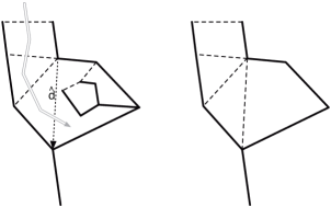
Figure 2: Identifying and processing a negative cycle. On the left, the tree $T$ is shown in solid. Non-tree edges are dashed. The unrelaxed dart $\hat{d}$ is dotted. The elementary cycle of $\hat{d}$ w.r.t. $T$ has negative length. The primal pushback path is double-lined gray. After the negative cycle is processed, its interior is deleted (on the right).

To control the number of pivots we initialize $T$ to have a property called right-shortness, and show it is preserved by the algorithm and that it implies that the number of pivots of any dart is bounded by the diameter of the graph. We later discuss how data structures enable the iterations to be performed efficiently.

4 Correctness and Analysis

We begin with a couple of basic lemmas. Consider the sink $t$ as the infinite face of ${G^{*}}$. By our conventions, any clockwise (counterclockwise) cycle $C$ in ${G^{*}}$ corresponds to a primal cut $(X,V-X)$ such that $t\in X$ ($t\notin X)$; see Fig. 1.

Lemma 1

Consider the sink $t$ as the infinite face of ${G^{*}}$. The length of any clockwise (counterclockwise) dual cycle does not decrease (increase) when flow is pushed to $t$. The length of any clockwise (counterclockwise) dual cycle does not increase (decrease) when flow is pushed from $t$.

Proof

The change in the length of a dual cycle is equal to the change in the residual capacity of the corresponding primal cut. Since clockwise cycles correspond to cuts $(X,V-X)$ s.t. $t\in X$, it follows that the residual capacity of a cut corresponding to a clockwise dual cycle can only increase when flow is pushed to $t$. The proofs of the other claims are similar.

The following is a restatement of a theorem of Miller and Naor [10].

Lemma 2

Let $G$ be a planar graph. Let $c_{0}$ be a capacity function on the darts of $G$. Let $f$ be a flow assignment. Define the length of a dart $d$ to be its residual capacity $c_{0}(d)-f(d)$. If $f$ is quasi-feasible then $f^{\prime}(d)=c_{0}(d)-\mbox{length}_{T}(d)$ is a feasible flow assignment, where $T$ is a shortest-path tree in $G^{*}$. Furthermore, $f^{\prime}=f+\phi$ for some circulation $\phi$.

Proof

Miller and Naor [10] proved that there exist a feasible circulation in $G$ if and only if ${G^{*}}$ contains no negative-length cycles when residual capacities in $G$ are interpreted as lengths in ${G^{*}}$. Furthermore, they proved that the flow assignment $\phi(d)=\mbox{length}(T[\text{head}_{G^{*}}(d)])-\mbox{length}(T[\text{tail}_{G^{*}}(d)])$ is such a feasible circulation in $G$.

Therefore, if $f$ is quasi-feasible then $\phi(d)$ is a feasible circulation with respect to the residual capacities $c(d)=c_{0}(d)-f(d)$. Thus, $c(d)-\phi(d)\geq 0$. Interpret $c(d)-\phi(d)$ as residual capacity with respect to some flow $f^{\prime}$ in $G$. Namely, $c(d)-\phi(d)=c_{0}(d)-f^{\prime}(d)$. Therefore, $f^{\prime}(d)=c_{0}(d)-c(d)+\phi(d)=f(d)+\phi(d)$. Furthermore,

$$f^{\prime}(d) = c_{0}(d)-c(d)+\phi(d)$$

$$= c_{0}(d)-c(d)+\mbox{length}(T[\text{head}_{G^{*}}(d)])-\mbox{length}(T[\text{tail}_{G^{*}}(d)])$$

$$= c_{0}(d)-\left(c(d)+\mbox{length}(T[\text{tail}_{G^{*}}(d)])-\mbox{length}(T[\text{head}_{G^{*}}(d)])\right)$$

$$= c_{0}(d)-\mbox{length}_{T}(d)$$

where the last equality follows from the definition of the reduced lengths with respect to $T$.

4.0.1 Correctness

To prove the correctness of the algorithm, we first show that an elementary cycle w.r.t. a back-edge is indeed a negative-length cycle.

Lemma 3

Let $\hat{d}$ be an unrelaxed back-edge w.r.t. $T$. The length of the elementary cycle of $\hat{d}$ w.r.t. $T$ is negative.

Proof

Consider the price function induced by from-root distances in $T$. Every tree dart whose tail is closer to the root than its head has zero reduced length. The reduced length of an unrelaxed dart is negative. Since $\hat{d}$ is a back edge w.r.t. $T$, its elementary cycle $C$ uses darts of $T$ whose length is zero. Therefore the reduced length of $C$ equals the reduced length of just $\hat{d}$, which is negative. The lemma follows since the length and reduced length of any cycle are the same.

Lemma 4

Let $C$ be the negative-length cycle defined in line 13. After $C$ is processed in line 14, $\mbox{length}(C)=0$ and $\hat{d}$ is relaxed. Furthermore, the following invariants hold just before line 14 is executed:

1. the flow pushed by the algorithm satisfies flow conservation at every node other than the sources (including super-sources) and the sink.

2. the outflow at the sources is non-negative.

3. there are no clockwise negative-length cycles.

Proof

The proof is by induction on the number of iterations of the main while loop of the algorithm. The initial flow pushed by the algorithm is from the sources to the sink. Therefore, conservation is satisfied at every non-terminal, the outflow at the sources is non-negative, and there is a one-to-one correspondence between over-saturated cuts in the primal and counterclockwise negative-length cycles in the dual.

For the inductive step, since by the inductive assumption there are no clockwise cycles, Lemma 3 implies that the cycle $C$ in line 13 must be counterclockwise. Therefore, the unrelaxed dart $\hat{d}$ in line 9 points in $\tau$ towards the root $t$. Thus, the length of $\hat{d}$ is increased in line 14 by $|\mbox{length}(C)|$, and the length of $C$ becomes zero. This shows the main claim of the lemma. To complete the proof of the invariants, note that the interior of $C$ is deleted in ${G^{*}}$, so the flow pushed in line 14 is now a flow from the sink to the newly created super-source. This shows that invariant (1) is preserved. Having $\mbox{length}(C)=0$ implies that the total flow pushed so far by the algorithm from the newly created super-source is non-negative. This shows (2).

Since the outflow at all sources is non-negative after the pushback, the inflow at the sink must still be non-negative and equals the sum of outflows at the sources. Therefore, for any negative-length dual cycle, the corresponding primal over-saturated cut $\Gamma(X)$ must be such that $t\notin X$. Hence any negative-length cycle is counterclockwise. This shows (3).

We now prove properties of the flow computed by the algorithm. The following lemma characterizes the flow recorded in line 16. Intuitively, this shows that it is a saturating feasible flow for the cut corresponding to the processed cycle.

Lemma 5

Let $C$ be a cycle currently being processed. Let $(X,V-X)$ be the corresponding cut, where $t\notin X$. Let $\vec{\delta}_{c}$ be the set of darts crossing the cut. The flow assignment $f$ computed in the loop in Line 16 satisfies:

1. $f(d)\leq c_{0}(d)$ for all darts whose endpoints are both in $X$.

2. every node in $X$ except sources and tails of darts of $\vec{\delta}_{c}$ satisfies conservation.

3. for every $d^{\prime}\in\vec{\delta}_{c}$, $\sum_{d:\text{head}(d)=\text{tail}(d^{\prime})}f(d)\geq\sum_{d\in\delta_{c}:tail(d)=tail(d^{\prime})}c_{0}(d)$

Proof

let ${G^{*}}_{c}$ denote the region of ${G^{*}}$ enclosed by $C$. Let $G_{c}$ denote the graph obtained from $G$ by contracting the sink side of $\Gamma_{c}$ into a single node. Note that ${G^{*}}_{c}$ is the dual of $G_{c}$. Let $\hat{d}$ be the non-tree dart of $C$. Since $\hat{d}$ is leafmost unrelaxed, there are no unrelaxed darts in ${G^{*}}_{c}$ other than $\hat{d}$. By Lemma 4, after the loop in line 14 is executed $\hat{d}$ is no longer unrelaxed as well. Therefore, the restriction of $T$ to ${G^{*}}_{c}$ is a shortest-path tree for ${G^{*}}_{c}$, and ${G^{*}}_{c}$ contains no negative cycles. The conditions of Lemma 2 are satisfied, so when $f(d)$ is set to $c_{0}(d)-\mbox{length}_{T}(d)$ in Line 16, it respects the capacities $c_{0}(d)$ for all $d\in G_{c}$. This shows 1.

By Lemma 4, just before $C$ is processed, the restriction of the flow pushed by the algorithm to $G_{c}$ satisfies conservation everywhere except at the sources and at the sink. In Line 14 flow is pushed back to $\text{tail}(\hat{d})$, so there is more flow entering $\text{tail}(\hat{d})$ than leaving it. Therefore, the restriction of the flow pushed by the algorithm to $G_{c}$ satisfies conservation everywhere except at the sources, the sink (which in $G_{c}$ is the only node outside $\Gamma_{c}$) and $\text{tail}(\hat{d})$. By Lemma 2, the flow $f(d)=c_{0}(d)-\mbox{length}_{T}(d)$ differs from the flow pushed by the algorithm by a circulation, so $f(\cdot)$ satisfies conservation at all those nodes as well.

In particular, for every dart $d^{\prime}\in\delta_{c}$, $0\leq\sum_{d:\text{head}(d)=\text{tail}(d^{\prime})}c_{0}(d)-\mbox{length}_{T}(d)$ (this is an inequality only for $d^{\prime}=\hat{d}$). However, note that the darts of $\delta_{c}$ are not strictly enclosed by $C$, and that $\mbox{length}_{T}(d)=0$ for every $d\in C$. Since Line 16 assigns $f(d)=c_{0}(d)-\mbox{length}_{T}(d)$ only to darts strictly enclosed by $C$ (and implicitly assigns zero to all other darts), we get that, for the darts of $\delta_{c}$, $0\leq\sum_{d:\text{head}(d)=\text{tail}(d^{\prime})}f(d)+\sum_{d\in\Gamma_{c}:\text{head}(d)=\text{tail}(d^{\prime})}c_{0}(d)$. Or alternatively, for every $d^{\prime}\in\Gamma_{c}$, $\sum_{d:\text{head}(d)=\text{tail}(d^{\prime})}f(d)\geq\sum_{d\in\Gamma_{c}:tail(d)=tail(d^{\prime})}c_{0}(d)$. This shows 2 and  3.

Lemma 6

The following invariant holds. In $G^{*}$ every source is enclosed by some zero-length cycle that encloses no negative-length cycles.

Proof

Initially, the face of $G^{*}$ corresponding to each source is such a cycle. At the time a cycle $C$ is processed and a super-source $s$ is created, $C$ is a zero-length cycle enclosing $s$ that encloses no negative-length cycles. The length of $C$ only changes if the pushback path ends at a dart of $C$ in the execution of Line 14 when processing a cycle $C^{\prime}$ at some later time. Since the interior of $C$ is deleted when $C$ is processed, $C^{\prime}$ encloses $C$. At this time, the interior of $C^{\prime}$, is contracted into a single new super-source which is enclosed by the zero-length cycle $C^{\prime}$ that encloses no negative cycles.

The following lemma is an easy consequence of lemma 6.

Lemma 7

The following invariant holds. There exists no feasible flow $f^{\prime}$ s.t. $\textrm{inflow}_{f^{\prime}}(t)$ is greater than $\textrm{inflow}_{f}(t)$, where $f$ is the flow pushed by the algorithm.

Proof

Let $f_{s}$ be the amount of flow source $s$ delivers to the sink in the flow pushed by the algorithm. Consider a flow $f^{\prime}$ and let $f^{\prime}_{s}$ be the amount of flow source $s$ delivers to the sink in $f^{\prime}$. By Lemma 6, at any time along the execution of the algorithm, every source is enclosed in a zero length cycle. Consider such a zero-length cycle $C$. If $\sum_{s\textrm{ enclosed by }C}f^{\prime}(s)>\sum_{s\textrm{ enclosed by }C}f(s)$ then the dual of the residual graph w.r.t. $f^{\prime}$ contains a negative cycle, so $f^{\prime}$ is not feasible.

Lemma 8

The flow $f$ computed in Line 18 is a maximum feasible flow in the contracted graph $G$ w.r.t. the capacities $c_{0}$.

Proof

The flow pushed by the algorithm satisfies conservation by Lemma 4. By Lemma 7, there is no feasible flow of greater value. Since there are no unrelaxed darts, $T$ is a shortest-path tree in ${G^{*}}$ and ${G^{*}}$ contains no negative cycles. Therefore, the flow pushed by the algorithm is quasi-feasible. This shows that the conditions of Lemma 2 are satisfied. It follows that $f$ computed in Line 18 satisfies conservation, respects the capacities $c_{0}$ and has maximum value.

Lemma 9

The flow assignment $f(d)$ is a feasible maximum preflow in the (uncontracted) graph $G$ w.r.t. the capacities $c_{0}$.

Proof

$f$ is well defined since each dart is assigned a value exactly once; in Line 16 at the time it is contracted, or in Line 18 if it was never contracted. By Lemma 8 and by part 1 of Lemma 5, $f(d)\leq c_{0}(d)$ for all darts $d$, which shows feasibility. By Lemma 8 and by part 2 of Lemma 5, flow is conserved everywhere except at the sources, the sink, and nodes that are tails of darts of processed cycles. However, for a node $v$ that is the tail of some dart of a processed cycle, $\sum_{d:head(d)=v}f(d)\geq 0$. This is true by part 3 of Lemma 5, and since $f(d)\leq c_{0}(d)$ for any dart. $f(\cdot)$ is therefore a preflow. Finally, the value of $f(\cdot)$ is maximum by Lemma 8.

Lemma 9 completes the proof of correctness since line 19 converts the maximum feasible preflow into a feasible flow of the same value.

4.0.2 Efficient implementation

The dual tree $T$ is represented by a table $\text{parentD}[\cdot]$ that, for each nonroot node $v$, stores the dart $\text{parentD}[v]$ of $T$ whose head in $G^{*}$ is $v$. The primal tree $\tau$ is represented using a dynamic-tree data structure such as self-adjusting top-trees [1]. Each node and each edge of $\tau$ is represented by a node in the top-tree. Each node of the top-tree that represents an edge $e$ of $\tau$ has two weights, $w_{L}(e)$ and $w_{R}(e)$. The values of these weights are the reduced lengths of the two darts of $e$, the one oriented towards leaves and the one oriented towards the root. The weights are represented so as to support an operation that, given a node $x$ of the top-tree and an amount $\Delta$, adds $\Delta$ to $w_{R}(e)$ and subtracts $\Delta$ from $w_{L}(e)$ for all edges $e$ in the $x$-to-root path in $\tau$.

This representation allows each of the following operations be implemented in $O(\log n)$ time: lines 9, 13, 11, 16, and 17, the loop of line 5, and the loop of line 14.

4.0.3 Running-Time Analysis

Lines 16 and 17 are executed at most once per edge. To analyze the running time it therefore suffices to bound the number of pivots in line 11 and the number of negative cycles encountered by the algorithm. Note that every negative length cycle strictly encloses at least one edge. This is because the length of any cycle that encloses just a single source is initially set to zero, and since the length of the cycle that encloses just a single super-source is set to zero when the corresponding negative cycle is processed and contracted.

Since the edges strictly enclosed by a processed cycle are deleted, the number of processed cycles is bounded by the number of edges, which is $O(n)$.

It remains to bound the number of pivots. We will prove that at the tree $T$ satisfies a property called right-shortness. This property implies that the number of times a given dart pivots into $T$ is bounded by the diameter of the graph.

Definition 1

[9] A tree $T$ is right-short if for all nodes $v\in T$ there is no simple root-to-$v$ path $P$ that is: as short as $T[v]$ and strictly right of $T[v]$

Since $T$ is initialized using right first search, initially, for every node $v$ there is no simple path in ${G^{*}}$ that is strictly right of $T[v]$. Therefore, initially, $T$ is right-short. The algorithm changes $T$ in two ways; either by making a pivot (line 11) or by processing a negative-length cycle (line 14). The following lemma was proved in [9]:

Lemma 10

[9] leafmost dart relaxation (line 11) preserves right-shortness.

Lemma 11

Right-shortness is preserved when processing the counterclockwise negative-length cycle $C$ in line 14.

Proof

For a node $v$, let $P$ be denote the tree path $T[v]$. Let $Q$ be a simple path that is strictly right of $P$. By right-shortness of $T$, before line 14 is executed $\mbox{length}(Q)>\mbox{length}(P)$. We show that this is also the case after line 14 is executed. By definition of right-of, $P\circ\mbox{rev}(Q)$ is a clockwise cycle. Note that since $C$ is counterclockwise, the changes in lengths of darts in line 14 correspond to pushing back flow from the sink $t$. Therefore, by Lemma 1, the length of $P\circ\mbox{rev}(Q)$ can only decrease. Since no dart of $P$ changes its length (only darts of $\tau$ are changed in line 14), this implies that $rev(Q)$ can only decreases in length. By antisymmetry, the length of $Q$ can only increase, so $\mbox{length}(Q)>\mbox{length}(P)$ after the execution as well.

We have thus established that

Corollary 1

$T$ is right-short at all times.

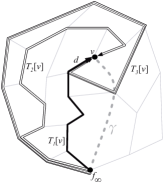
Figure 3: Bounding the number of pivots of dart $d$ whose head is a node $v$ of ${G^{*}}$. Three tree paths to $v$ at times $t_{1}<t_{2}<t_{3}$ are shown. $T_{3}[v]$ (triple-lined) is left of $T_{2}[v]$ (double-lined) and $T_{2}[v]$ is left of $T_{1}[v]$ (black) . The dart $d$ is in $T_{1}[v]$ and $T_{3}[v]$, but not in $T_{2}[v]$. Therefore, it must have pivoted out of $T$ and into $T$ between time $t_{1}$ and $t_{3}$. The curve $\gamma$ (dashed) visits only nodes of ${G^{*}}$. The winding number of $T_{1}[v]$ about $\gamma$ is 0. The winding number of $T_{3}[v]$ must be greater than that of $T_{1}$ (1 in this example).

Consider a dart $d$ of ${G^{*}}$ with head $v$. Let $\gamma$ be an arbitrary root$(T)$-to-$v$ curve on the sphere. Let $T_{1}[v]$ and $T_{2}[v]$ denote the tree path to $v$ at two distinct times in the execution of the algorithm. Since right-shortness is preserved throughout the algorithm and since with every pivot $\mbox{length}(T[v])$ may only decrease, if $T_{2}[v]$ occurs later in the execution than $T_{1}[v]$, then $T_{2}[v]$ is left of $T_{1}[v]$. It follows that the winding number of $T[v]$ about $\gamma$ between any two occurrences of $d$ as the pivot dart in line 11 must increase. See Fig. 3. Therefore, if we let $T_{0}$ denote the initial tree $T$, and $T_{t}$ denote the tree $T$ at the latest time node $v$ appears in ${G^{*}}$, then the number of times $d$ may appear as the pivot dart in line 11 is bounded by the difference of the winding numbers of $T_{t}[v]$ and $T_{0}[v]$ about $\gamma$. Since $\gamma$ is arbitrary, we may choose it to intersect the embedding of ${G^{*}}$ only at nodes, and to further require that it visit the minimum possible number of nodes of ${G^{*}}$. This number is bounded by the diameter of the face-vertex incidence graph of $G$, which is bounded by the minimum of the diameter of $G$ and the diameter of ${G^{*}}$. Since both $T_{0}$ and $T$ are simple, the absolute value of their winding number about $\gamma$ is trivially bounded by the number of nodes $\gamma$ visits. Therefore, the total number of pivots is bounded by $\sum_{d}\textrm{diameter}=O(\textrm{diameter}\cdot n)$. The total running time of the algorithm is thus bounded by $O(\textrm{diameter}\cdot n\log n)$.

References

- [1] S. Alstrup, J. Holm, K. de Lichtenberg, and M. Thorup. Maintaining information in fully dynamic trees with top trees. ACM Transactions on Algorithms, 1(2):243–264, 2005.
- [2] G. Borradaile and P. N. Klein. An algorithm for maximum -flow in a directed planar graph. Journal of the ACM, 56(2), 2009.
- [3] G. Borradaile, P. N. Klein, S. Mozes, Y. Nussbaum, and C. Wulff-Nilsen. Multiple-source multiple-sink maximum flow in directed planar graphs in near-linear time. 2011. Submitted.
- [4] Y. Boykov and V. Kolmogorov. An experimental comparison of min-cut/max-flow algorithms for energy minimization in vision. IEEE Transactions on Pattern Analysis and Machine Intelligence, 26:1124–1137, September 2004.
- [5] M. R. Henzinger, P. N. Klein, S. Rao, and S. Subramanian. Faster shortest-path algorithms for planar graphs. Journal of Computer and System Sciences, 55(1):3–23, 1997.
- [6] G. F. Italiano, Y. Nussbaum, P. Sankowski, and C. Wulff-Nilsen. Improved algorithms for min cut and max flow in undirected planar graphs. In Proceedings of the 43rd Annual ACM Symposium on Theory of Computing, 2011. To appear.
- [7] D. B. Johnson and S. Venkatesan. Using divide and conquer to find flows in directed planar networks in time. In Proceedings of the 20th Annual Allerton Conference on Communication, Control, and Computing, pages 898–905, 1982.
- [8] H. Kaplan and Y. Nussbaum. Maximum flow in directed planar graphs with vertex capacities. In Proceedings of the 17th European Symposium on Algorithms, pages 397–407, 2009.
- [9] P. N. Klein. Multiple-source shortest paths in planar graphs. In Proceedings of the 16th Annual ACM-SIAM Symposium on Discrete Algorithms, pages 146–155, 2005.
- [10] G. L. Miller and J. Naor. Flow in planar graphs with multiple sources and sinks. SIAM Journal on Computing, 24(5):1002–1017, 1995. preliminary version in FOCS 1989.
- [11] J. Reif. Minimum - cut of a planar undirected network in time. SIAM Journal on Computing, 12:71–81, 1983.
- [12] A. Schrijver. On the history of the transportation and maximum flow problems. Mathematical Programming, 91(3):437–445, 2002.
- [13] H. Whitney. Planar graphs. Fundamenta mathematicae, 21:73–84, 1933.