The luminosity–dependent high–redshift turnover in the steep spectrum radio luminosity function: clear evidence for downsizing in the radio-AGN population

Abstract

This paper presents a new grid–based method for investigating the evolution of the steep–spectrum radio luminosity function, with the aim of quantifying the high–redshift cut–off suggested by previous work. To achieve this, the Combined EIS–NVSS Survey of Radio Sources (CENSORS) has been developed; this is a 1.4 GHz radio survey, containing 135 sources complete to a flux density of 7.2 mJy, selected from the NRAO VLA Sky Survey (NVSS) over 6 deg² of the ESO Imaging Survey (EIS) Patch D. The sample is currently 73% spectroscopically complete, with the remaining redshifts estimated via the $K$–$z$ or $I$–$z$ magnitude–redshift relation. CENSORS is combined with additional radio data from the Parkes All–Sky, Parkes Selected Regions, Hercules and VLA COSMOS samples to provide comprehensive coverage of the radio power vs. redshift plane. The redshift distributions of these samples, together with radio source count determinations, and measurements of the local luminosity function, provide the input to the fitting process.

The modelling reveals clear declines, at $>3\sigma$ significance, in comoving density at $z>0.7$ for lower luminosity sources ($\log P=25-26$); these turnovers are still present at $\log P>27$, but move to $z\mathrel{\lower 2.58334pt\hbox{$\buildrel{\textstyle>}\over{\scriptstyle\sim}$}}3$, suggesting a luminosity–dependent evolution of the redshift turnover, similar to the ‘cosmic downsizing’ seen for other AGN populations. These results are shown to be robust to the estimated redshift errors and to increases in the spectral index for the highest redshift sources.

Analytic fits to the best–fitting steep spectrum grid are provided so that the results presented here can be easily accessed by the reader, as well as allowing plausible extrapolations outside of the regions covered by the input datasets.

1 Introduction

It has become increasingly apparent in recent years that radio–loud active galactic nuclei (AGN) play a key role in galaxy evolution; the interplay of their expanding radio jets and the surrounding intergalactic and intracluster medium acts to provide part, or possibly all, of the heat required to prevent both large–scale cluster cooling flows and the continued growth of massive ellipticals (e.g. Fabian et al., 2006; Best et al., 2006; Best et al., 2007; Croton et al., 2006; Bower et al., 2006). Determining the evolution of the radio luminosity function (RLF) is therefore important for understanding the timescales on which they impose these effects. Also, since radio–loud AGN are powered by the most massive black holes, their RLF can be used to investigate the behaviour of the upper end of the black–hole mass function and hence the build–up of these objects in the early Universe.

The work of Sandage (1972); Osmer (1982); Peacock (1985); Schmidt et al. (1988), and in particular Dunlop & Peacock (1990, hereafter DP90), has shown that the comoving number density of both flat and steep–spectrum powerful radio galaxies, selected at 2.7 GHz, is greater by two to three orders of magnitude at a redshift of two compared with the present day Universe. This density increase is expected to peak at some point simply because sufficient time is needed for their host galaxies to grow into the massive ellipticals, with correspondingly large central black holes, that are typically observed for radio–loud AGN (e.g. Best et al., 1998). This high–redshift ‘cut off’ was seen by Peacock (1985) in the flat–spectrum population and was also detected in the steep–spectrum population by DP90 beyond $z\sim 2.5$; but their results were limited by the accuracy of the photometric redshifts from their faintest radio–selected sample, so they were not able to quantify the decline. It should also be noted that the DP90 work assumed an Einstein–de Sitter cosmology which means that the high redshift sources in their sample were ascribed lower luminosity than for a $\Omega_{\rm\Lambda}>0$ cosmology, thus potentially making a cut–off easier to find.

Following DP90, Shaver et al. (1996) reported evidence of a sharp cut–off in space density in their sample of flat–spectrum radio sources. However, this result was disputed by Jarvis & Rawlings (2000) who showed that it could be caused by an increasing curvature of the spectral indices with redshift, and that a shallower decline was more consistent with the data. A more rigorous analysis of radio–loud quasars by Wall et al. (2005), using a larger sample, confirmed a decrease in the number density of flat–spectrum sources at $z\mathrel{\lower 2.58334pt\hbox{$\buildrel{\textstyle>}\over{\scriptstyle\sim}$}}3$.

A shallow space density decline between $z\simeq 2.5$ and $z\simeq 4.5$ was also found in low–frequency–selected steep–spectrum sources by Jarvis et al. (2001), although a constant density value was also consistent with their data; their sample lacked the depth needed for firm results. Waddington et al. (2001) used a deeper survey and saw evidence that the turnover for lower–luminosity sources appeared to occur at lower redshift than that of brighter flux–limited samples. They were also able to discount some of the DP90 models, but their study lacked the volume needed for better measurements of the space density changes of powerful radio sources. Indications of a similar luminosity dependence of the cut–off redshift were also seen for radio–loud Fanaroff & Riley (1974) class I (FRI) sources by Rigby, Snellen & Best (2008).

The evolution of radio–selected AGN can be linked to the behaviour of AGN selected in other bands. For example the space density of optically–selected quasi–stellar objects (QSOs) shows a strong decrease at $z>2.1$ (Boyle et al., 2000; Fan, 2001; Wolf et al., 2003; Fan, 2004), consistent with that found for both radio–loud (Wall et al., 2005), as well as X–ray selected quasars (Hasinger et al., 2005; Silverman et al., 2005). There is also evidence for a luminosity–dependent redshift cut–off in the optical and X–ray selected QSO samples (Ueda et al., 2003; Hasinger et al., 2005; Richards et al., 2005; Wall, 2008). Since radio–loud QSOs are thought to correspond to flat spectrum sources (e.g. Barthel, 1989; Antonucci, 1993), investigating the evolution of the flat and steep populations can result in a new understanding of the links between radio–loud (quasars and radio galaxies) and radio–quiet (QSOs) sources. A full review of radio–loud AGN evolution can be found in De Zotti et al. (2010).

To properly investigate the evolution of the steep spectrum RLF it is clear that a combination of several radio surveys of differing depth is needed to ensure a broad coverage of the radio luminosity–redshift (P–z) plane. In particular, faint radio samples are needed if the $z\mathrel{\lower 2.58334pt\hbox{$\buildrel{\textstyle>}\over{\scriptstyle\sim}$}}2$ behaviour is to be determined. This has motivated the development of the 150–object, 1.4 GHz selected, Combined EIS–NVSS Survey of Radio Sources (CENSORS; Best et al., 2003, hereafter Paper I), which has been designed to maximise the information for high–redshift, steep–spectrum, radio sources close to the break in the RLF.

In this paper the CENSORS dataset, combined with additional samples, is used to investigate the nature of the high–redshift evolution of radio sources, via a new grid–based modelling technique in which no prior assumptions are made about the behaviour of the luminosity function. This is an improvement on previous investigations which have either used functional forms, or only considered pure luminosity or density evolution, or a combination of both (although Dye & Eales 2010 have recently developed a similar method to study the evolution of sub–mm galaxies).

The layout of the paper is as follows: Section 2 describes both CENSORS and the additional data sets needed; Section 3 presents the modelling technique; Section 4 describes the results from the best–fitting model and investigates their robustness; finally Section 5 summarises the findings. Throughout this paper values for the cosmological parameters of H${}_{0}=70$ km s^-1Mpc^-1, $\Omega_{\rm m}=0.3$ and $\Omega_{\rm\Lambda}=0.7$ are used and the spectral index, $\alpha$ is defined as $S_{\nu}\propto\nu^{-\alpha}$.

2 Input data

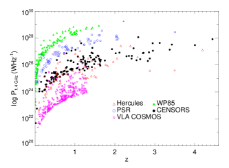
Figure 1: The Wall & Peacock (1985, WP85), Parkes Selected Regions (PSR, Downes et al. 1986, Dunlop et al. 1989), CENSORS, Hercules (Waddington et al., 2001) and VLA COSMOS (for $z\leq 1.3$ only; Smolčić et al., 2008) samples plotted on a radio–luminosity vs. redshift plane to illustrate how they efficiently cover a large part of the plane without much overlap. Radio luminosities were calculated using previously published spectral indices for the WP85, PSR and Hercules samples; $\alpha=0.8$ was assumed for the sources in VLA–COSMOS. The spectral indices for the CENSORS sample are taken from Ker et al. (2011). The PSR, WP85 and COSMOS samples are restricted to steep spectrum sources only. See text for full details of sample selection.

As discussed above, several data sets are needed to constrain the radio source cosmic evolution. In addition to the CENSORS sample, therefore, four other radio samples, along with determinations of the local radio luminosity function, and measurements of the radio source counts are used; these are described in this section. Fig. 1 illustrates the coverage of the P–z plane obtained using these radio samples.

Table 1: Key information relating to the five radio samples used in the modelling. $N({\rm total})$ gives the total number of sources in each sample as used here; $N(z_{\rm spec})$, $N(z_{\rm photo})$, $N(z_{\rm est})$ and $N(z_{\rm limit})$ give the number of sources with spectroscopic, photometric, estimated (via either the $K$–$z$ or $I$–$z$ relations) or lower limit $K$–$z$ redshifts respectively.

Name	1.4 GHz Limit (Jy)	Sky Area (sr)	$N({\rm total})$	$N(z_{\rm spec})$	$N(z_{\rm photo})$	$N(z_{\rm est})$	$N(z_{\rm limit})$
WP85	4.0	9.81	83	79	–	4	–
PSR	0.30	0.075	74	41	–	30	3
CENSORS	0.0072	0.0018	135	99	–	31	5
Hercules	0.002	0.00038	64	42	19	1	2
VLA-COSMOS	0.0001	0.00036	314	–	314	–

2.1 CENSORS

The full CENSORS sample contains 150 sources with $S_{\rm 1.4GHz}>3.8$ mJy in a 3 by 2 deg field of the ESO Imaging Survey (EIS) Patch D, centred on 09 51 36.0, $-$21 00 00 (J2000). Best et al. (2003, Paper I) present the radio data, along with the optical host galaxy identifications, with additional $K$–band imaging presented by Brookes et al. (2006, Paper II). Spectroscopic data for a subset of the sample can be found in Brookes et al. (2008, Paper III), which also gives estimated redshifts for the remainder of the sample, calculated using the K–z and, for one source, the I–z magnitude–redshift relations.

Since the publication of Papers I–III some small reassessments have been made to the sample. Subsequent radio data have shown that:

• CENSORS 66 and CENSORS 82 are actually the lobes of a FRII radio source whose host galaxy is located at 09 50 48.97, $-$21 32 55.8 (Gendre, priv. comm.), with a $K$–band magnitude of 17.8 $\pm$ 0.1 in a 4.5 arcsec diameter aperture ($K=18.2\pm 0.1$ when corrected to the standard 63.9 kpc diameter aperture; see Paper II for details) and $I=21.7\pm 0.1$. This results in an estimated K–z redshift of 1.40 (calculated using $\log z=0.0025K^{2}+0.113K-2.74$; cf. Paper III);

• similarly, CENSORS 84 and CENSORS 85 are also the lobes of an extended double radio source, whose host galaxy is located at 09 55 36.87, $-$21 27 12.5, with a $K$–band aperture corrected magnitude of 13.1 $\pm$ 0.2 and a corresponding estimated $K$–$z$ redshift of 0.15;

• the host galaxy of CENSORS 64 is located at 09 49 01.60 $-$20 50 00.7 (Ker et al., 2011) with $K$ and $I$ band magnitudes of 15.04 $\pm$ 0.08 (when aperture corrected) and 17.44 $\pm$ 0.02 respectively with a corresponding estimated redshift of 0.33. This compares well to its new spectroscopic redshift of 0.403 (Ker et al., 2011).

Spectral indices for the sources, calculated using the new radio data, will be presented in Ker et al. (2011), but are also included here in the analysis of Fig. 3.

Additional $K$–band imaging was obtained for 14 sources using IRIS2 (in service mode) on the Anglo–Australian Telescope. As a result of this, the host galaxy of CENSORS 69 has now been detected, with a $K$–band magnitude of 20.1 $\pm$ 0.3 (19.6 $\pm$ 0.3 when aperture corrected). New spectroscopic data subsequently showed it to have a redshift of 4.01 (Ker et al., 2011). Finally, the $K$–$z$ limits presented in Paper II were discovered to be in error and have been recalculated. The correct values and corresponding new $K$–$z$ redshift limits, along with the new IRIS2 $K$–band data, can be found in Appendix B, within the up–to–date CENSORS dataset.

Of the original 150 CENSORS sources, 135 are deemed to be complete to a flux density limit of 7.2 mJy, and it is this subset which is used in this paper. No other selection is performed, meaning that it contains both starforming galaxies along with steep– and flat–spectrum sources. The current host galaxy identification fraction of this is 96% with a spectroscopic completeness of 73%. Table 1 summarises the salient information for this subsample.

2.2 The Wall & Peacock 2.7 GHz radio sample

The sample of Wall & Peacock (1985, hereafter WP85) includes the brightest radio sources at 2.7 GHz over an area of 9.81 sr, and is complete to 2 Jy. The original paper presents redshifts for 171 of the 233 source sample, and a further 20 were added by Wall & Peacock (1999). Since then further spectroscopic observations have been published by a variety of groups, raising the redshift completeness to 98%. As part of the back-up programme for CENSORS two of the WP85 sources, 0407-65 and 1308-22, have been observed with FORS2 on the VLT (see Appendix A). The redshift measured for 0407-65 is in good agreement with that observed by Labiano et al. (2007), but the observation of 1308-22 updates the redshift estimate quoted in McCarthy et al. (1996). For the remaining two sources without useful spectra, the estimated redshifts of Wall & Peacock (1985) are used. There is an excess of sources in this sample at $z<0.1$, some of which may be contaminating starburst galaxies, so a minimum redshift of 0.1 is imposed here; doing this does not degrade the analysis as this region of parameter space will be well constrained by the local radio luminosity function.

Complete spectral indices are available for this sample making it straightforward to convert the 2.7 GHz flux densities to 1.4 GHz; since it is only the behaviour of the steep–spectrum luminosity function which the model will assess (as discussed in Section 3) only steep spectrum WP85 sources are considered in this.

In order to use this sample in the modelling of the RLF it needs to be converted into a sample with an effective 1.4 GHz flux density limit. To do this, a flux limit of $S_{\rm 1.4GHz}=4$ Jy was adopted, corresponding to a spectral index $\alpha=1.06$ for sources at the 2.7 GHz limit. It is possible that sources with a steeper spectral index than this may be below the WP85 sample flux limit at 2.7 GHz and still have a 1.4 GHz flux density above 4 Jy, thus leading to incompleteness in the sample. A search was therefore carried out for such sources, so they could be added to the sample. In the Northern Hemisphere this is simple as there is a fainter ($S_{\rm 2.7GHz}\geq 1.5$ Jy) sample from Peacock & Wall (1981) covering the WP85 area; this contains one source with a flux lower than 2 Jy, but a corresponding 1.4 GHz value above 4 Jy (and $z\geq 0.1$). In the Southern Hemisphere there are two 408 MHz surveys, the Best et al. (2003) equatorial sample and Burgess & Hunstead (2006), which between them cover the rest of the WP85 survey region. Since these are lower frequency surveys, any such steep spectrum sources will be bright and can be identified. Searching these samples reveals two $z\geq 0.1$ steep–spectrum sources brighter than 4 Jy at 1.4 GHz, but not in the WP85 sample. Oddly, calculating the 2.7 GHz flux densities of these sources reveals that they should have been detected by WP85. It is not clear why they were missed, but it is possible that they have very curved spectra. The data for these three ‘missing’ sources are given in Table 2, whilst Table 1 summarises the WP85 sample as used in this paper (including the three sources discussed above); the full dataset can be found in Appendix C.

Table 2: The additional sources that were added into the WP85 sample to correct for incompleteness. The $z_{\rm ref}$ gives the reference for the redshift – G05 for Grimes et al. (2005) or BH06 for Burgess & Hunstead (2006).

Name	$S_{\rm 2.7GHz}$	$S_{1.4\rm GHz}$	$\alpha$	$z$	$z_{\rm ref}$
	(Jy)	(Jy)
3C325	1.84	4.29	1.29	1.135	G05
Name	$S_{\rm 408MHz}$	$S_{1.4\rm GHz}$	$\alpha$	$z$	$z_{\rm ref}$
	(Jy)	(Jy)
1526–423	17.86	5.08	1.02	0.5	BH06
1827–360	25.83	6.49	1.12	0.12	BH06

2.3 The Parkes Selected Regions 2.7 GHz radio sample

The Parkes Selected Regions (PSR; Wall et al. 1968, Downes et al. 1986, Dunlop et al. 1989) cover 0.075 sr in six 6.5^∘ square fields of view down to a flux density limit of 0.1 Jy at 2.7 GHz. The updated sample of Dunlop et al. (1989) presents redshifts for 82 of the 178 sources in the sample and subsequent observations published by a variety of groups result in a further 24 redshifts. Of the remaining 72 sources, 10 have estimated values from Dunlop & Peacock (1993), whilst the remainder were estimated using the K–z relation as outlined for the CENSORS sources in Paper III. The $K$–band photometry for the sample (Dunlop et al., 1989) uses 12.4^′′diameter apertures for most objects. These are large enough such that aperture corrections are sufficiently small to be ignored. Where a $K$–band magnitude is not available one is estimated via the relation: $K=-1.1(B-R)+18.3$ (Dunlop et al., 1989). Two sources have been omitted from this sample due to unclear identification and non–detection.

The current PSR dataset suffers from some incompleteness below 0.15 Jy, becoming quite large by 0.1 Jy (DP90) so there is also a desire to minimise the contribution of these faintest sources. The 1.4 GHz flux density limit is therefore set at 0.3 Jy to achieve this. All 2.7 GHz sources with a 1.4 GHz flux density greater than this are included in the final sample; the lowest of these has a 2.7 GHz value of 0.14 Jy which should be sufficiently above the incompleteness limit to avoid problems. Table 1 summarises the PSR sample as it used in this paper, whilst the full dataset can be found in Appendix C.

2.4 The Leiden–Berkeley Deep Survey Hercules sample

The Leiden–Berkeley Deep Survey covers 5.52 sq. deg. over nine high latitude fields, and was originally based upon multi–colour plates from the 4 m Mayall telescope at Kitt Peak (Kron 1980; Koo & Kron 1982) alongside Westerbork Synthesis Radio Telescope 1.4 GHz radio observations (Windhorst et al., 1984). One of these fields, in the constellation of Hercules, has subsequently been followed up by Waddington et al. (2000, 2001; see also ), who defined a complete sample of 64 radio sources (both starforming galaxies and steep and flat–spectrum objects) with $S_{\rm 1.4GHz}>2$ mJy within 1.2 sq. degrees. The spectroscopic redshift completeness of the sample is 66% [41 redshifts measured by Waddington et al. 2001 with one additional value from Rigby, Snellen & Best 2007]. Of the remaining 22 sources, 20 have photometric redshifts also from Waddington et al. (2001) but the final two only have estimated K–z lower limits due to host galaxy non–detections. Table 1 summarises the salient information for the Hercules sample, whilst the full dataset can be found in Appendix C.

2.5 The AGN subsample of the VLA COSMOS survey

Smolčić et al. (2008) defined a sample of 601 AGN with z $\leq$ 1.3 in the 2 deg² COSMOS field using the multiwavelength imaging available for the region. The redshift limit was imposed because beyond this the AGN/star–forming galaxy separation becomes unreliable, leading to possible contamination of the sample. The radio sensitivity varies with position across the field, but over a well–defined area of 1.17 deg² it is possible to define a clean sample complete to S${}_{\rm 1.4GHz}\geq$ 100 $\mu$Jy; this contains 314 steep spectrum sources. Robust photometric redshifts were calculated for the survey and are available for all of these sources. Table 1 summarises the salient information for the VLA COSMOS sample; however, unlike the other samples, this full dataset is not available in Appendix C as it is still proprietary, and was obtained via private communication with the authors.

2.6 Source counts data

Any model of RLF evolution must match the measured radio source counts as a function of flux density and so this comparison will also be used in the modelling process. The data used for this were taken from Bondi et al. (2008), Seymour et al. (2004), Windhorst et al. (1984), White et al. (1997) and Kellermann & Wall (1987) to ensure that a sufficient range of flux densities (0.05 mJy – 94 Jy) was covered. The White et al. counts are limited to $S_{\rm 1.4GHz}>2$ mJy only, as they note that they are incomplete below this. The full set of 1.4 GHz source counts used in the modelling can be found in Appendix C and the counts themselves are shown in Fig. 7, within the discussion of the modelling results (Section 4.1).

2.7 Local radio luminosity functions

The local radio luminosity function (LRLF) for AGN was measured by Sadler et al. (2002) using the 2dF galaxy redshift survey (2dFGRS; Colless 1999, Colless et al. 2001), by Best et al. (2005, 2011), using the Sloan Digital Sky Survey (SDSS; York et al. 2000), and by Mauch et al. (2007) using the 6 degree Field Galaxy Survey (6dFGS DR2 Jones et al. 2004). Sadler et al. (2002) compiled their LRLF from a sample of all 2dFGRS, NVSS selected radio galaxies with $z\leq 0.3$. Note that while the 2dFGRS LRLF includes points at $\log P_{1.4\rm{\,GHz}}=25.9\text{~{}and~{}}26.3$ (as converted to the cosmology used here) these are not included due to the small number (1) of sources in each band. Best et al. (2011) use the seventh data release of the SDSS, combined with the NVSS and FIRST 1.4 GHz radio surveys (using a similar process to that carried out by Best et al. (2005) for the second data release, but now with an independent normalisation), to produce a sample of 9168 radio sources, with a median redshift of $\sim\!\!$  0.1. Similarly the Mauch et al. (2007) LRLF was calculated using the 7824 NVSS radio sources contained in the second incremental data release of the 6dFGS; the median redshift for their sample is 0.043. In addition, 95% confidence upper limits are added at the highest radio luminosities ($\log P_{1.4{\rm\,GHz}}>27.0$) as no sources were detected at these luminosities in the three datasets. The LRLF data used in the modelling can be found in Appendix C.

3 Modelling technique

Unlike previous attempts to model the evolution of the RLF (e.g. Dunlop & Peacock 1990, Jarvis et al. 2001, Willott et al. 2001, etc.), no assumptions are made about the shape of the luminosity functions here. Instead, they are determined by allowing the densities, $\rho$, at various points on a $P$–$z$ grid of radio luminosities and redshifts to each be free parameters and then simply finding the best–fitting values to this many–dimensional problem. The $P$–$z$ grid points were chosen so as to allow sensitive calculations to be made without having so many parameters involved that finding a best fit becomes a prohibitively long task (but with more powerful computers and larger datasets the technique could be expanded to sample much finer detail). The range of radio luminosities covered was $\log P_{1.4{\rm\,GHz}}=19.25\rm{~{}to~{}}29.25$, equally spread in steps of 0.5 in $\log P_{1.4{\rm\,GHz}}$. Densities were evaluated at the redshifts 0.1, 0.25, 0.5, 1.0, 2.0, 3.0, 4.0, 6.0. The $\rho$ at any $(P,z)$ can then be interpolated from the nearest four grid points, except at $z<0.1$ where the densities are assumed to be constant (see Section 3.1 below).

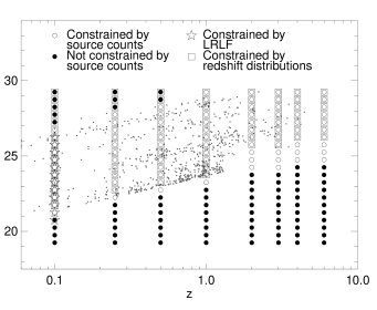
Figure 2: The various regions of the $P$–$z$ plane that are constrained by the redshift distributions, the source counts and the local radio luminosity function (LRLF). The redshift distribution constraint is determined by the COSMOS sample at $z\leq 1.3$ and the Hercules sample above this, as they are the deepest surveys; the positions of the individual sources in the five samples are shown as grey dots. The source counts cover the $S$–$z$ grid used in the modelling process, which takes a lower limit of 0.1 mJy and an upper limit of 50 Jy.

The $P$–$z$ plane is constrained by the samples described in Section 2. This is demonstrated in Fig. 2, which highlights the different regions which are covered by different data types. The densities that are actually included in the fitting process are those that are constrained by the faintest redshift distribution or the source counts; grid points that are unconstrained are excluded. As Fig. 2 shows, high–redshift, low–luminosity sources do not satisfy this criterion and are therefore not included in the modelling. The total number of points fitted, and hence the dimensions of the minimisation process, is 101.

The amoeba algorithm for downhill simplex minimisation (Nelder & Mead 1965) is used to obtain the best fitting space densities. It takes as input a set of parameters and a scaling factor and uses these to construct a geometrical object of $N+1$ points in $N$ dimensions called a simplex. It uses a user–defined function to calculate the likelihood of each vertex of the simplex, and then reflects, contracts or expands these vertices until the function is minimised. In order to achieve this best fit in reasonable time, the algorithm was run in a multi-stage loop with varying scaling and tolerance for the first five steps. The maximum number of iterations allowed within amoeba for each stage is set to 3000 and the process ends when the likelihood ratio of successive stages is less than 1.0000001.

The subsections below describe the calculation of the input modelling parameters, along with an explanation of the likelihood calculation used.

3.1 Construction of the input density grids

Three $P$–$z$ grids are used as inputs to the modelling program containing the source densities for steep–spectrum, flat–spectrum and star–forming populations separately (the total radio source space density obviously being the sum of these three at any grid point). Considering these three grids separately is essential since the five different radio source samples used in the modelling include and exclude different populations, as well as on the good physical grounds that the different populations might well evolve differently. As the aim of this work is to investigate the evolution of the radio galaxy RLF, the star–forming grid is fixed. Its inclusion is necessary as the low flux densities of the CENSORS and Hercules samples mean that radio emission from star formation becomes significant. The flat–spectrum radio–source grid is also held constant since the low numbers of this type of source in the input samples do not allow minimisation; more accurate constraints come from previous surveys explicitly targetting these sources.

The star–forming grid is created by evolving the local star–forming galaxy luminosity function of Sadler et al. (2002) such that

$$\Phi\left(P,z\right)=\begin{cases}\Phi\left(\frac{P}{\left(1+z\right)^{2.5}},0\right)&z\leqq z_{\rm max},\\ \Phi\left(\frac{P}{\left(1+z_{\rm max}\right)^{2.5}},0\right)&z>z_{\rm max}.\end{cases}$$ (1)

where $\Phi$ is the comoving density of radio sources due to star formation, $P$ and $z$ are the luminosity and redshift respectively, and $z_{\rm max}$ is the redshift where the space density plateaus. The power law index of 2.5 is taken from Smolčić et al. (2009) who studied star forming galaxies in VLA–COSMOS out to $z\sim 3$; their value agreed with that previously found by Seymour et al. (2004). The value $z_{\rm max}=2$ is adopted, following Blain et al. (1999), but its precise value is irrelevant to this work as the contribution of star forming galaxies at $z>1$ is negligible at the flux densities studied.

Similarly, the starting steep–spectrum grid (which the minimisation then varies) is formed by evolving the Sadler et al. (2002) local AGN RLF by $(1+z)^{3}$ in density. Conversely, the flat–spectrum grid is created by taking the median value from the results of the seven evolutionary models presented in DP90, after conversion to the cosmology used here. This is in broad agreement with the recent results of Wall et al. (2005), and minor variations are not critical given that this population is small compared to steep–spectrum sources.

An $S$–$z$ (flux density–redshift) grid is, in many cases, more readily compared with real data than the $P$–$z$ grid, as it can be converted easily into source numbers. The modelling code therefore uses the three $P$–$z$ grids to populate three corresponding $S$–$z$ grids containing 120 flux density bins covering the range 0.1 mJy–50 Jy at 1.4 GHz, equally spaced in $\log$ S, and 300 redshift bins covering the range 0–6, equally spaced in $z$. This $z$–range is wider than that previously used to define the $P$–$z$ grid in order to cover the full range of the radio samples. To account for this, two extra bins – $z=0.001$ and $z=0.05$ – are inserted into the $P$–$z$ grids. For the steep spectrum grid, the densities for these additional grid points are assumed to be constant with redshift, and are therefore set to the $z=0.1$ values; for the flat–spectrum and star forming grids they are calculated from the input models. For a given $P$–$z$ grid the density at a given point on the $S$–$z$ grid $\rho(S,z)$, is found by linear interpolation of the density values from the four surrounding points in the expanded $P$–$z$ grid. The total number of sources per steradian in each bin is then given by:

$$N(S,z)=\rho(S,z)\frac{dV}{dz}d(\log S)dz.$$ (2)

The star forming and flat–spectrum $S$–$z$ grids are only calculated once as they are not changed in the minimisation process. The steep spectrum $S$–$z$ grid is recalculated in each cycle of the amoeba process as $\rho(S,z)$ changes when $\rho(P,z)$ changes. Although the source counts extend to lower flux densities, it is not useful to extend the modelled region because source counts alone do not provide a sufficient constraint on the radio luminosity functions.

3.1.1 Spectral index selection

Figure 3: The changes in spectral index with redshift for the steep–spectrum sources in the four radio samples with measured $\alpha$ values. Also shown is the relation from Ubachukwu et al. (1996) which follows the datapoints reasonably well. The spectral indices were calculated using 1.4 GHz to 0.6 GHz, 1.4 GHz to 5 GHz, 2.7 GHz to 5 GHz and 1.4 GHz to 325 MHz flux densities for the Hercules, PSR, WP85 and CENSORS samples respectively.

The calculation of the appropriate luminosity for a given flux density and redshift bin in the $S$–$z$ grid requires a value for the spectral index, $\alpha$. For the flat–spectrum and star–forming grids, $\alpha$ is assumed to be 0.0 and 0.8 respectively; the small contribution of these populations means that a more precise value is not necessary. However, the steep–spectrum spectral index may vary with redshift and luminosity, which could significantly alter the results. This $P$–$z$–$\alpha$ degeneracy means that either parameter could be used to give the $\alpha$ variation. Unlike DP90, who adopted a $P$–$\alpha$ relation, it is the redshift dependence which is used here for the steep–spectrum grid; Ker et al. (2011) will investigate these spectral index variations in more detail. The default form for this variation is taken from Ubachukwu et al. (1996) who found that the mean spectral index increases with redshift as $\alpha=0.83+0.4\log(1+z)$; as Fig. 3 shows, this relation gives a reasonable approximation to the available steep–spectrum sample data, with a possible over–estimation of $\alpha$ at high redshift. The CENSORS spectral indices in particular would also be consistent with a flat relation, but this may be because they are low frequency, making them appear flatter than the high frequency WP85 and PSR values. Section 4.3.1 considers the effects other $\alpha$ assumptions, including a constant value, have on the modelling, though it should be noted that reasonable variations in $\alpha$ do not lead to qualitative differences in the results.

In addition to this, a Gaussian scatter in $\alpha$ of 0.2 is also incorporated at each redshift in the steep–spectrum grid to account for any variations in the value within a redshift bin; this is a reasonable assumption given the spread seen in Fig. 3. In practice this is implemented by creating 21 versions of the $S$–$z$ grid, extending to $\pm 2.5\sigma$ (in steps of $0.25\sigma$), which are each assigned a weight depending on how far they are away from the mean. Redshift bins where $\alpha<0.5$ are ignored (as sources within them would not be in the steep spectrum sample) and their weight evenly distributed over the remainder. The $P$–$z$ grid densities, $\rho(P,z)$, corresponding to each $(S,z)$ point are then interpolated onto the bins in these 21 new $S$–$z$ grids as before; the final grid carried forward into the minimisation is their weighted sum.

Table 3: The grids used for each dataset comparison in the modelling process. ‘steep’, ‘stars’ and ‘flat’ indicate the grids for steep–spectrum, star–forming and flat–spectrum grids respectively. Note that it is only the steep–spectrum grid which is allowed to vary in the modelling process.

Dataset	Comparison grid
	$P$–$z$	$S$–$z$
VLA–COSMOS		steep
Hercules		steep+stars+flat
CENSORS		steep+stars+flat
PSR		steep
WP85		steep
LRLFs	steep+flat
Source counts		steep+stars+flat

Figure 4: The redshift distributions for the five samples, CENSORS, Hercules, WP85, PSR and VLA–COSMOS, included in the modelling. The histograms are plotted with a binsize of 0.2 in $z$ and incorporate the uncertainties arising from the limits and estimated redshifts by representing them as weighted Gaussian distributions (see Section 3.2 for details). The overplotted solid lines show the model predictions for each sample, and the bin shading shows the contribution from the different redshift determinations. For samples which were compared to some combination of the three input grids, the contributions from the additional grids are also shown separately to illustrate the dominance of the steep spectrum population at high redshift. See Table 3 for information on which grids were used for each dataset.

3.2 Comparing the model predictions to data

The input data from the redshift distributions of the five different radio source samples described in Section 2, along with the local RLF and the observed source counts, now need to be compared to the model grids described in the previous Section. To do this, the model local RLFs are simply read from the appropriate ($z=0.1$) column in the $P$–$z$ grid, and the model redshift distributions, $N(z,S_{\rm limit})$ for some sample with survey area $A$ and flux limit $S_{\rm limit}$, and source counts, $N(S)$, are easily calculated from the $S$–$z$ grid using

$$N(z,S_{\rm limit})=A\times\sum_{S>S_{\rm limit}}{N(S,z)}$$ (3)

and

$$N(S)=\sum_{z}N(S,z)$$ (4)

respectively. Different datasets are compared to different combinations of the model grids, depending on their content. For instance, the sum of the steep and flat spectrum $P$–$z$ grids is fitted to the LRLF data as they were created using only AGN, but the source counts are compared against the sum of all three $S$–$z$ grids as they include starforming galaxies. Table 3 summarises which of the grids are used for comparison to each dataset.

A $\chi^{2}$–test, $\chi^{2}=\sum_{i}{\frac{(O_{i}-E_{i})^{2}}{\sigma^{2}}}$, is used to assess the model predictions for each dataset in turn. For the source counts and the local radio luminosity function, the data points and their uncertainties provide the values of $O$ and $\sigma$. It is impractical, given the large number of data points involved (and the wish to add more as they become available) to choose model grid points that exactly match the locations (flux density or luminosity) of the data, and therefore the values of $E$ are calculated by interpolating between neighbouring model grid points. The $\chi^{2}$ comparison also includes a term for the upper limits on the high radio luminosity points in the LRLF; this is done by setting the ‘data’ points for these luminosities equal to zero and setting the corresponding errors equal to the upper limit of the LRLF.

When comparing the model predictions with the redshift distributions, it is important to note that there are insufficient sources at the high–redshift end of the redshift distributions (a part of the parameter space that is of particular interest) to formally allow a $\chi^{2}$–test to be used. A possible solution to this would be to carry out a source–by–source likelihood analysis instead, calculated using the product of the model prediction for the redshift probability distribution at the redshift of each of the sample sources; this returns the maximum likelihood value if the data exactly match the model distribution. A problem with this method, however, is the difficulty of accounting for the uncertain redshifts present in several of the samples.

An alternative solution is therefore adopted here, by matching the shape of the redshift distributions using polynomial fits, and comparing these with the model predictions. The smoothing that this provides at high redshifts mitigates the issue of small source numbers in the high–redshift bins. It also helps to lessen anomalous features in the redshift distributions, such as the drop in source numbers at $z\sim 1.5$ in the CENSORS, Hercules and PSR samples (Fig. 4). The latter arises because of the onset of the ‘redshift desert’, where spectroscopic redshifts are difficult to obtain: the $K$–$z$ estimates should fill this gap, but in practice the scatter in the $K$–$z$ relation, combined with the lack of spectroscopic measurements, means there is a overall bias for redshifts to lie outside of this region.

The polynomials are fitted to histograms with binsizes of 0.1 in $z$, beginning at $z=0.0$, with the exception of WP85, which, as discussed previously in Section 2.2, has a minimum redshift of 0.1. Additionally, the VLA COSMOS sample was only defined to $z=1.3$ (due to lack of AGN/star–formation separation beyond that redshift) so no fitting is allowed beyond this. Once the value of a polynomial fit reaches zero it is set to zero for all subsequent redshifts, to prevent it returning negative source numbers. The order of polynomial selected for each redshift distribution is the one that gives the minimum reduced chi–squared – 6 for CENSORS, Hercules and COSMOS, 3 for PSR and 4 for WP85 – and these input fits are shown in Fig. 4.

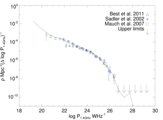
Figure 5: The data for the three input LRLFs used in the modelling process (points) along with the best–fitting model LRLF prediction (solid line) from the $z=0.1$ column in the combined steep and flat spectrum final $P$–$z$ grids.

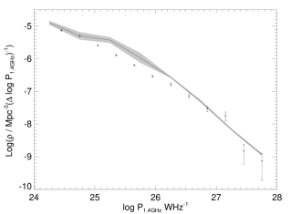
Figure 6: The source count data used in the modelling process (points) along with the best–fitting prediction for the counts from the three final model $S$–$z$ grids (solid line). Also shown are the contributions to the model counts for the steep–spectrum (dotted line), flat spectrum (dashed line) and starforming galaxies (dot–dashed line) separately to illustrate the dominance of the steep population.

Figure 7: The RLF data points of Donoso et al. (2009) compared to the best–fitting model prediction at $z=0.5$ from the steep–spectrum grid (solid line). The shaded region shows the $5\sigma$ confidence limits of the model.

The polynomial fitting takes into account the uncertainty from both estimated and photometric redshifts present in these datasets, by representing each source as a Gaussian distribution centred on the given redshift, with the width equal to either the published photometric redshift error, or, for the $K$–$z$ estimates, 0.14 in $\log z$ (the 1$\sigma$ spread in the 7C $K$–$z$ relation (Willott et al. 2003)). The $K$–$z$ limits can similarly be modelled, but are assigned a width (in $\log z$) of 0.4 above and 0.1 below the given value to represent their increased uncertainty (see Paper III for more discussion). This distribution is then included in the redshift histograms, thus spreading the source across different redshift bins, depending on the errors. The effect of these redshift uncertainties on the modelling results are investigated, in Section 4.3.2, by changing these assumptions.

The polynomial fits are then compared to the model predictions using a $\chi^{2}$–test, with the polynomial values providing the $E$ parameters in these equations, evaluated at redshifts and flux densities which match points in the model grid, and the $O$ values given by the model prediction at those grid points. The corresponding $\sigma$ values are taken as the uncertainty in the polynomial value, generated from the covariance matrix of the polynomial fit coefficients.

Using polynomial fits to represent the redshift distributions in this way has one drawback: although the fitting method should return the correct minimum point, and thus identify the correct best–fit model grid, the absolute value of $\chi^{2}$ at that point will not necessarily be a true measure of the goodness–of–fit of the model. This is because the polynomial–derived errors are correlated. Any scaling error in $\chi^{2}$ will then lead to a mis-estimate of the uncertainties on the model predictions (see Section 3.3). To account for this, the $\chi^{2}$ values derived using the polynomial-fit method for the best-fit model prediction were compared with ‘true’ $\chi^{2}$ values. The latter were derived by comparing the best-fit model with the observed source numbers in different redshift bins, but with all estimated redshifts treated as exact, and the bin sizes increased to ensure that each redshift bin contained a minimum of 5 sources; this avoids problems with small number statistics, but means that resolution is lost at the high–redshift end. This analysis showed that the polynomial-fit method provided values of $\chi^{2}$ which were a factor $f=0.3$ away from the true value. The $\chi^{2}$ values from the redshift distributions are therefore scaled by this factor in order to ensure that accurate uncertainties are determined.

The scaled $\chi^{2}$ values are transformed to likelihoods, and combined to produce an overall measure of the goodness of the fit:

$$L=\exp\left(\frac{-\chi_{\rm LRLF}^{2}}{2}\right)\exp\left(\frac{-\chi_{\rm counts}^{2}}{2}\right)\exp\left(\frac{-f\chi_{\rm z-dists}^{2}}{2}\right),$$ (5)

which is then returned to the minimisation routine amoeba.

3.3 Constraint in the $P$–$z$ grid

It is not sufficient to find the best fit to the data without obtaining some measure of the uncertainty associated with each point on the $P$–$z$ grid. In this section the intrinsic modelling limits offered for the constraint of the $P$–$z$ grid are presented, whilst the effect of uncertainty in the input data is discussed later in Sections 4.3.1 and 4.3.2.

Assuming an ideal data set, uncertainty still arises due to the degeneracy across parameters in the model. The conditional error for parameter $p$ is given by:

$$\sigma_{\rm cond,p}^{2}=\left(-\frac{\partial^{2}\ln L}{\partial p^{2}}\mid_{\rm peak}\right)^{-1}.$$ (6)

In practice it is determined by finding the value of the parameter for which $\ln L(p)-\ln L(\hat{p})=0.5$, from which $\sigma=\rho(p)-\rho(\hat{p})$. This is then a measure of the uncertainty in a given parameter whilst holding all other parameters constant.

However the actual uncertainty may be greater when the variation of other parameters is taken into account. This is the marginalized error and comes from the diagonal of the inverse Hessian matrix, $H$, where:

$$\sigma_{\rm marg,i}^{2}=\left[H\right]_{\rm i,i}^{-1},$$ (7)

for parameter i, where,

$$H_{\rm i,j}=\frac{\partial^{2}\ln L}{\partial p_{\rm i}\partial p_{\rm j}}.$$ (8)

This is calculated here via the finite difference approximation (note that diagonal terms in the Hessian matrix are simply $-1/\sigma_{\rm cond,p}^{2}$). It is these marginalized errors that are quoted in the results presented in the remainder of this paper. In general these are comparable to the conditional errors, but for some grid points they are up to a factor of two higher.

4 Results and discussion

This Section presents the best–fitting steep–spectrum $P$–$z$ grid produced by running the modelling code described in Section 3 above, and examines how well its predictions agree with the input datasets. The best–fitting $P$–$z$ grid and its associated error is given in full in Appendix D.

4.1 Dataset comparison

Figure 8: The individual model steep–spectrum radio luminosity functions vs. redshift from the best–fitting $P$–$z$ grid (solid lines). Points are only plotted here if they are constrained by at least two of the input datasets (see Fig. 2 for details). Also shown are the median of the evolutionary models from DP90 (dashed lines).

The success of the best-fitting steep spectrum $P$–$z$ grid, combined where necessary with the unvaried flat spectrum and starburst grids, at fitting the input data is illustrated in Figs 4 to 7 for the five sample redshift distributions, the LRLF, and the differential source counts respectively. The agreement with both the LRLF and the source counts is very good – this is to be expected for two reasons. The constraint provided by the LRLFs is tight and particular to specific parameters, meaning that the model has little freedom to vary it. At the opposite extreme, there are numerous combinations of densities which will satisfy the observed counts, as they depend on the summation carried out across the $P$–$z$ grid to transform it to $S$–$z$. Thus, whilst fitting these data is essential, on their own they do not provide a particularly interesting constraint. The source counts comparison plot (Fig. 7) also breaks down the model prediction into the different contributions from the three populations; this shows that the steep–spectrum sources dominate at the flux densities probed by the current samples, which in turn justifies limiting the fitting to them only at this point.

The redshift distributions also derive from the $S$–$z$ grid so they prevent nonsensical combinations of densities fitting the source counts, and the stronger constraint that they provide is therefore essential to obtaining information about the evolution of the luminosity function. Again the flat and starburst populations are plotted separately in Fig. 4 where relevant, showing their small contribution, especially at the high redshifts which are of particular interest here.

The model predictions for all five samples are generally in good agreement with the data across the whole of each redshift range. The total numbers of sources given by the model are 131.1, 67.7, 74.5, 284.8 and 84.5 for CENSORS, Hercules, PSR, COSMOS and WP85 respectively; these are well matched to the actual figures of 135, 64, 74, 314 and 83.

As a further check on the results, the final model grid can also be compared to datasets that were not included in the fitting: for example the $\bar{z}=0.55$ radio luminosity function determined by Donoso et al. (2009) using a sample of $\sim$14000 radio–loud AGN, created by combining the NVSS and FIRST 1.4 GHz radio surveys with the MegaZ–LRG catalogue; this comparison is shown in Fig. 7. The match is reasonable over the luminosity range of the data, and the overprediction seen at $25<\log P<26$ is likely to be because Donoso et al. were only considering radio sources associated with luminous red galaxies in their sample, and therefore miss any bluer radio galaxies (this is also why this sample was not included as an explicit constraint).

4.2 Model luminosity functions

Fig. 8 shows the behaviour of the individual best–fitting steep–spectrum luminosity functions with $z$ for $\log P=25.25$ to $\log P=27.75$ inclusive, averaged over bins of 0.5 in $\log P$. This luminosity range was chosen as it covers the region of the $P-z$ plane with the most constraints as illustrated in Fig. 2; additionally, high redshift points are only plotted if they are constrained by both the redshift distributions and the source counts. Also plotted as a comparison is the median of the seven evolutionary models calculated by DP90 (translated to the cosmology used for this work), which all suggest a mild high redshift decline in the number density of sources of these powers.

The evolving luminosity function (in which the grid densities are plotted against $\log P$ for different redshifts) is shown in Fig. 9. As before regions of radio power and redshift are excluded if they are not constrained by at least two datasets. Displaying the grid behaviour in this way is a useful alternative to Fig. 8 as it gives an overview of the space density changes with radio power and redshift.

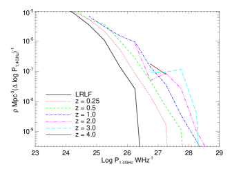
Figure 9: The evolving luminosity function. Points are only plotted here if constrained by more than one dataset and errors have been ignored for clarity.

The low–$z$, $\log P\geq 26.5$ points are discrepantly low (albeit with large error bars) compared to their neighbours. This is a result of the weaker constraints provided by the upper limits of the LRLF to the minimisation process (though this region is also constrained by the source counts and redshift samples). Inspection of Fig. 7 (the combined LRLF from the steep and flat spectrum grids) illustrates that the model reaches well below the upper–limits of the densities in these regions. Similarly, there are some apparently anomalous high redshift points (e.g. the ‘dip’ seen at $z\sim 2$ for $26.5<\log P<27$ and the $z=3$ points at $\log P<26.5$); Figs 2 and 1 suggest that although these should be constrained by both the redshift distributions and the source counts, the low densities are likely to result from a lack of sources in the radio samples covering this range. However, the ‘dip’ in particular may not just be the result of low–number statistics as it lies within the ‘redshift desert’ discussed previously in Section 3.2.

4.3 The high–redshift turnover

Inspection of Figs 8 shows that decreases in space density are present to some degree at $z\mathrel{\lower 2.58334pt\hbox{$\buildrel{\textstyle>}\over{\scriptstyle\sim}$}}0.5$ for all the luminosities considered. At low powers these declines are clear and occur at $z\sim 1$, but at the highest powers the densities remain essentially level with no strong decline, out to $z\sim 4$. The agreement with the DP90 results is reasonable, though visually there seems to be a trend for the low power cutoffs to be at lower redshifts than DP90, and the high power cutoffs to be at higher redshift. However, the range in the DP90 results, and the inability to probe the full distance range for these low powers, means it is difficult to draw firm conclusions about the differences.

The ‘strength’ of the cut–off, $C_{\sigma}$, between the density at the peak redshift, $\rho_{\rm peak}$ and that at any of the $n$ subsequent redshift points can be quantified as:

$$C_{\sigma}=\frac{\rho_{\rm peak}-\rho_{\rm peak+n}}{\sqrt{(}\sigma_{\rm peak}^{2}+\sigma_{\rm peak+n}^{2})},$$ (9)

where $\sigma_{\rm peak}$ and $\sigma_{\rm peak+n}$ are the corresponding errors on the peak and post–peak space densities. However, caution is necessary when calculating $C_{\sigma}$ for the results presented here, because of the discrepant, badly constrained, points discussed in the previous Section. The quantised nature of the grid also means that it is often relatively flat after the peak, before dropping sharply. To minimise these effects, $\rho_{\rm peak+n}$ is taken as the average of the space densities at redshifts higher than the peak position. This average is weighted by the available volume in each redshift bin, and the $z=6$ point is ignored in all cases due to the lack of supporting data in the redshift distributions. The error, $\sigma_{\rm peak+n}$, for this average density is calculated by combining the post–peak space density errors in quadrature, taking the volume weighting into account. The results of this calculation are shown in Table 4; they support the previous observation that the declines are strong for the faintest powers, but tend to be weaker at brighter powers.

Table 4: The redshift at the grid point at which the space density is highest, $z_{\rm grid}$, and the strength of the cut–off, $C_{\sigma}$following that point from the average of the post–peak densities (excluding the $z=6$ points), using Equation 9. Also shown is the peak redshift, $z_{\rm fit}$, determined from the polynomial fitting described in Section 4.3. The different versions illustrate the effects of altering various model parameters; see Section 4.3.1 and 4.3.2 for full details.

Radio power range	$z_{\rm grid}$	$z_{\rm fit}$	$C_{\sigma}$
Default: $\alpha=0.83+0.4\log(1+z)$
25.00 – 25.50	0.5	0.7	3.8
25.50 – 26.00	1.0	1.1	9.6
26.00 – 26.50	1.0	1.4	5.6
26.50 – 27.00	4.0	2.3	–
27.00 – 27.50	3.0	2.6	0.7
27.50 – 28.00	3.0	3.9	10.0
$\alpha=0.8+0.25z$
25.00 – 25.50	1.0	0.8	–
25.50 – 26.00	1.0	1.2	2.4
26.00 – 26.50	1.0	1.4	4.0
26.50 – 27.00	2.0	1.6	2.1
27.00 – 27.50	4.0	2.6	–
27.50 – 28.00	3.0	3.2	5.9
$\alpha=1.5$
25.00 – 25.50	1.0	0.7	–
25.50 – 26.00	0.5	0.7	1.5
26.00 – 26.50	1.0	1.4	4.8
26.50 – 27.00	1.0	1.4	4.0
27.00 – 27.50	4.0	2.8	–
27.50 – 28.00	2.0	2.3	11.4
$\alpha=0.8$
25.00 – 25.50	0.5	0.7	2.4
25.50 – 26.00	1.0	0.9	7.9
26.00 – 26.50	1.0	1.4	16.1
26.50 – 27.00	4.0	2.5	–
27.00 – 27.50	2.0	1.9	6.7
27.50 – 28.00	3.0	3.8	6.5
Average strength from 50 random variations of the redshift limits
25.00 – 25.50	0.5	0.7	1.8
25.50 – 26.00	1.0	1.0	8.6
26.00 – 26.50	1.0	1.4	2.6
26.50 – 27.00	4.0	2.1	–
27.00 – 27.50	3.0	2.6	0.2
27.50 – 28.00	3.0	4.0	9.8
Uncertain $z$ at $+1\sigma$
25.00 – 25.50	1.0	0.8	–
25.50 – 26.00	1.0	1.3	6.5
26.00 – 26.50	1.0	1.4	6.7
26.50 – 27.00	2.0	1.8	5.9
27.00 – 27.50	3.0	2.5	4.4
27.50 – 28.00	3.0	3.6	15.5
Uncertain $z$ at $-1\sigma$
25.00 – 25.50	0.5	0.7	3.5
25.50 – 26.00	1.0	1.2	3.1
26.00 – 26.50	1.0	1.3	5.0
26.50 – 27.00	1.0	2.3	2.4
27.00 – 27.50	3.0	2.1	1.1
27.50 – 28.00	3.0	3.8	4.6

Fig. 8 and Table 4 both show an apparent luminosity–dependence of the peak redshift, $z_{\rm peak}$, but the wide redshift bins in the $P$–$z$ grid means the position of the peak is ambiguous. For a better estimate, polynomials (generally of order 2, but also of order 3 where necessary) were fitted to the model steep–spectrum $\rho$–$z$ distributions, for various radio power bins, with the aim of roughly parametrizing this $z_{\rm peak}$ vs $\log P$ relation. Fig. 10 shows the results of this for the best–fitting steep spectrum grid, with error bars showing the uncertainties in the polynomial fit. Also shown is the range in $z_{\rm peak}$ found from repeating this fitting for the different spectral indices and redshift limits discussed in Sections 4.3.1 and 4.3.2. This is not a rigorous analysis but it does illustrate the general increase in $z_{\rm peak}$ over the radio luminosity range probed.

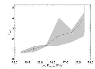
Figure 10: An illustration of the changes in peak redshift with radio power for the best–fitting steep–spectrum grid (solid line). The error bars show the uncertainty in the polynomial fits and the shaded region represents the range in results which come from repeating this process for the additional grids in Sections 4.3.1 and 4.3.2.

4.3.1 The effect of the spectral index

The creation of the $S$–$z$ grid, used in the modelling for the data from the five samples and source counts, requires a value for the spectral index, $\alpha$. The choice of $\alpha$ is complicated by the spectral curvature seen in some radio–loud sources (e.g. Laing & Peacock 1980), which can result in an increase in the spectral indices at higher redshift (see Jarvis & Rawlings 2000 for a discussion of this effect for flat–spectrum sources); as Fig. 3 shows, this effect is seen in the radio samples used here, albeit with a large scatter. Ignoring this may lead to under–estimation of the high–$z$ space density (and increase the significance of any density cut–off) since the steepest spectrum sources are missed. In the modelling results presented in the previous Section attempts were made to take this into account by using the $\alpha$–$z$ relation from Ubachukwu et al. (1996) in the creation of the $S$–$z$ grid. This provides a reasonable match to the data (Fig. 3) but it is important to investigate the effect a different choice has on the high–redshift behaviour of the model RLFs. Changing the assumed value of $\alpha$ will move sources into different radio power bins and hence strengthen some turnovers, and weaken others.

Fig. 11 presents the results of using both an extreme spectral index of 1.5, and a stronger increase with redshift (arbitrarily modelled as $\alpha=0.8+0.25z$ to give ultra–steep spectra at $z\mathrel{\lower 2.58334pt\hbox{$\buildrel{\textstyle>}\over{\scriptstyle\sim}$}}2$). Note that these will represent extreme cases since some radio sources with typical $\alpha\sim 0.8$ spectra are found at high redshift (e.g. Jarvis et al. 2009). The cut–off strengths are also given in Table 4. In both cases the general effect is to increase the densities at $z\mathrel{\lower 2.58334pt\hbox{$\buildrel{\textstyle>}\over{\scriptstyle\sim}$}}0.3$, and weaken the high–redshift cut–off, as sources in the $S-z$ grid have moved into higher radio power bins. Overall this is a good illustration of how far $\alpha$ needs to be increased to reduce the significance of the cut–offs to the $\sim 3\sigma$ level. Also shown, as a comparison, is the effect of using $\alpha=0.8$, the low–redshift mean value; this generally decreases the densities but the decline is still present at high significance for all powers.

Figure 11: The effect on the steep–spectrum model luminosity functions of changing the value of the spectral index, $\alpha$ for three luminosity ranges. The ‘$\alpha=0.83+0.4\log(1+z)$’ line comes from the best fitting model grid presented earlier. Larger bins of $\Delta\log P=1$ are shown to better illustrate how the changes affect the results. In all cases a scatter of $\alpha\pm 0.2$ around the mean value was also included, as previously discussed in Section 3.1.

4.3.2 The effect of the redshift incompleteness

The other uncertainty in the model results comes from the estimated redshifts and redshift limits present to some degree in the five input samples. Attempts are made to take these into account in the modelling process, but this is likely to be less successful for the $z$–limits as their true value is less constrained. To investigate what effect this has, the model was run 50 times; in each run each limit is assigned a new, higher, redshift, drawn randomly from a uniform 10000 element distribution, starting at the given limit, up to a maximum of $z=6$. As a further check the modelling was repeated with all the uncertain redshifts, both estimates and limits, moved up and down by $1\sigma$. No other attempt is made to account for the uncertainty in the estimated redshifts and limits in either of these cases.

Figs 12 and 13 show the spread in densities resulting from this, and the cut–off strengths can be found in Table 4. They show that whilst the turnover is preserved in both cases, it is generally strengthened at moderate powers when all the uncertain redshifts are shifted by $\pm 1\sigma$, compared with the original results, because sources are shifted out of these regions to higher power and redshift bins. When the redshift limits are randomly increased the turnover is weakened due to sources being moved into the higher redshift bins.

Figure 12: The effect on the steep–spectrum model luminosity functions of repeatedly randomly moving the redshift limits to a new, higher, value, up to a maximum of $z=6$. For this the estimated redshifts were kept at their given values, with no attempt to take their uncertainties into account as done previously. ‘default’ in the Fig. labels refers to the original modelling results presented in Section 4.2. Larger bins of $\Delta\log P=1$ are shown to better illustrate how the changes affect the results. In all cases an error of $\alpha\pm 0.2$ was also included, as previously discussed in Section 3.1.

Figure 13: The effect on the steep–spectrum model luminosity functions of moving the estimated redshifts and redshift limits up and down by their $1\sigma$ values (these were taken as $+$0.4 and $-$0.1 for the limits); no other attempt is made to take the redshift uncertainties into account. The ‘$\alpha=0.83+0.4\log(1+z)$’ line comes from the best fitting model grid presented earlier. Larger bins of $\Delta\log P=1$ are shown to better illustrate how the changes affect the results. In all cases an error of $\alpha\pm 0.2$ was also included, as previously discussed in Section 3.1.

4.4 Testing the robustness of the redshift turnover

The excellent coverage of the $P$–$z$ plane in the range $26<\log P<28$ to $z\sim 5$, demonstrated in Fig. 1 and 2, allows a further test of how robust the redshift cut–offs seen in Fig. 8 are to possible incompleteness in the radio samples. This is done by determining the number of fake high–redshift radio sources that need to be inserted into this luminosity range to reduce the cut–off strength to $<3\sigma$. In practice this was split into two parts because of the changing position of the cut–off with luminosity and the range of the different samples. Firstly, different numbers of new Hercules sources, with redshifts and luminosities randomly selected from $2.5<z<4$ and $26<\log P<27$, were inserted and the modelling repeated. Next, Hercules was returned to its original composition and the process repeated for CENSORS, but this time with extra sources drawn from $3.5<z<6$ and $27<\log P<28$. The number of real sources in these two redshift ranges (2.2 in Hercules, 2.6 in CENSORS, incorporating the spread in estimated redshifts as described in Section 3.2) is well reproduced by the polynomial fits used to represent the data, which give 3.0 and 4.2 sources respectively, so adding fake sources in this way should give a good indication of the number needed to significantly affect the turnover.

Table 5 gives the resulting cut–off strengths for the average density following the peak; it indicates that the number of CENSORS or Hercules sources in these ranges has to approximately double to push the significance of the cut–off below 3$\sigma$. It should also be noted that these numbers are likely to be a lower limit, as the modelling is likely to overpredict the number of real sources at these redshifts. This is because of the input polynomial used for the fitting, which typically underestimates at lower redshifts, thus leading to overestimation at $z\mathrel{\lower 2.58334pt\hbox{$\buildrel{\textstyle>}\over{\scriptstyle\sim}$}}3$.

Both the CENSORS and Hercules samples contain sources without host galaxy identifications or with no spectroscopic redshifts, so the extra sources required to remove the turnovers could simply be missing. However, this possibility has already been considered in Section 4.3.2, where it was shown that moving all estimated redshifts to their upper limits does not remove the space density declines.

An alternative determination of the number of fake sources required to remove the redshift turnovers in these radio power and redshift ranges can be made by freezing the relevant high–redshift space densities at their peak values, and then calculating the total number of sources that would have been detected in the CENSORS or Hercules samples in the absence of a decline in density. These numbers – 11.7 for Hercules and 12.4 for CENSORS – are comparable to the total number of sources present in these bins with the addition of the fake sources discussed earlier in this Section.

Table 5: The cut–off strength for the average redshift point following the peak for $26<\log P<27$ and $2.5<z<4$ and $27<\log P<28$ and $3.5<z<6$ for the addition of different numbers of fake sources, $N(\rm fake)$ into the Hercules and CENSORS sample respectively. The $N(\rm fake)=0$ value is for the original version of the redshift samples.

	Hercules	CENSORS
$N(\rm fake)$	$C_{\sigma}$	$C_{\sigma}$
0	6.5	5.0
1	3.0	3.6
2	2.9	2.5
3	2.3	3.0
4	1.1	2.9
5	0.6	2.2
6	1.0	1.5
7	0.1	1.2

4.5 Polynomial approximation of the best–fit $P$–$z$ grid

The usefulness of the best–fit $P$–$z$ grid (given in Appendix D) to the reader is limited, because it only varies smoothly in regions where it is covered by the available data. To improve this situation the whole grid is fit four times with a fourth order polynomial series expansion, similar to the one used for the DP90 models. This provides an easy method to calculate the space density values at any $(z,P)$ point, as well as allowing extrapolations of the data to regions currently not well constrained.

The basic polynomial series used for the fit is:

$$\log~{}\rho=\Bigg{(}\sum_{i=0}^{4}{{\sum^{4-i}_{j=0}A_{ij}x(P)^{i}y(z)^{j}}}\Bigg{)}+Bx^{5}y^{5},$$ (10)

where $x$ and $y$ represent the radio power and redshift axes of the grid respectively. Only points constrained by two of the input datasets are used in this fitting. The $z=6$ points are also excluded as the uncertainties in this region are large. The co–efficients for the four different versions of this fit are given in Appendix D. These were chosen to give several extensions into the unconstrained region, and the only difference between them is the co–ordinates used for $x$ and $y$:

• Fit 1: $x=\log P$, $y=\log z$

• Fit 2: $x=\log P$, $y=\log(1+z)$

• Fit 3: $x=0.1(\log P-20)$, $y=\log z$

• Fit 4: $x=0.1(\log P-20)$, $y=\log(1+z)$ .

The results of the fits for one radio power range are shown in Fig. 14 (the full set of plots for $\log P=25.25$ to $\log P=27.75$ inclusive can also be found in Appendix D) and the agreement with the best–fit grid is good. However, it should be stressed that this smooth version of the grid is not a perfect representation of the model output and this is why it was not used for the analyses in the previous subsections.

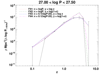
Figure 14: The results of the four smooth fits to the $P$–$z$ grid for one radio power range. The full set of plots for $\log P=25.25$ to $\log P=27.75$ inclusive can also be found in Appendix D).

5 Summary and conclusions

The results presented in this paper demonstrate that the method of RLF determination described here works well; it gives an easy means of estimating errors and hence assessing the robustness of any evolutionary behaviour seen, such as the presence of a redshift turnover. Examination of the best–fitting steep–spectrum $P$–$z$ grid suggests that the turnover in the radio luminosity function occurs at $z\simeq 0.7$ for the faintest luminosities considered here, and then moves to $z\mathrel{\lower 2.58334pt\hbox{$\buildrel{\textstyle>}\over{\scriptstyle\sim}$}}2$ for higher powers. These changes are consistent with those seen for steep–spectrum radio sources by Waddington et al. (2001) who found turnovers in redshift at $z\simeq 1$ for low–luminosity sources ($P_{\rm 1.4GHz}>10^{25.1}$ W/Hz) but at $z\simeq 2$ for the more powerful ($P_{\rm 1.4GHz}>10^{26-27}$ W/Hz). Similarly a redshift peak at $z\simeq 2$ for the brightest sources is also seen for flat–spectrum quasars, in radio–loud, optical and X–ray selected samples (e.g. De Zotti et al. 2010, Wall 2008, Hasinger et al. 2005, Richards et al. 2005). They are also in broad agreement with the assumption of a low luminosity peak at $z=0.706$, and a high luminosity peak at $z=1.91$, in the simulations of Wilman et al. (2008), which make predictions for the next generation of radio telescopes. The results presented here nevertheless suggest that a luminosity–dependent peak, with a high–redshift decline, would be a better representation of the real data than the two population model, with a flat post–peak space density, that these simulations currently adopt.

Physically, the luminosity dependence of the redshift peak in the radio galaxy RLF suggests that the most massive black holes have formed by $z\simeq 4$ and that their lower mass counterparts formed later. This ‘cosmic downsizing’ may initially appear to be at variance with the hierarchical model of structure formation. However, this discrepancy can be solved if the mode of AGN fuelling changes with cosmic time: in the early Universe major mergers provide the cold gas to power the accretion at high rates, but at lower redshift it is low–luminosity, radiatively inefficient accretion from hot gas haloes that dominates (Fanidakis et al. 2010).

The datasets available for this work mean that only a narrow range in luminosity is constrained well enough to draw firm conclusions about the luminosity function evolution. Better coverage of the $P$ –$z$ plane will improve this. However, the density turnovers are robust and remain present even in the unlikely scenario that all the estimates are 1 $\sigma$ higher or lower. The turnovers seen in this work are also in good agreement with the work of Wall et al. (2005) who find a cut–off at a significance level $>4\sigma$ for their sample of flat spectrum quasars.

The agreement with the DP90 results seen at high redshift for the brightest luminosities is not surprising; this region is dominated by CENSORS sources, which have already been shown to be consistent with two of their models (Paper III), both of which include a redshift cut–off.

The modelling method presented here can be easily modified to investigate different populations separately. The modelling results in this paper are limited by the uncertain redshifts present in some samples and further spectroscopic observations for the CENSORS sample are ongoing to improve this situation. Future increases in sample size would allow independent minimisation of all three grids, as well as subdividing the grids further into additional populations, e.g. Fanaroff & Riley Class I and II galaxies (Fanaroff & Riley 1974), or high and low excitation line radio sources (e.g. Hardcastle et al. 2006). The upcoming large, deep radio surveys from both the LOw Frequency ARray (LOFAR) and the Australian Square Kilometre Array Pathfinder (ASKAP) will be ideal for this, but complementary redshift data, using the deep multicolour optical photometry from the planned Large Synoptic Survey Telescope (LSST) for example, is essential. Such an extension of this work would yield an invaluable tool for investigating the links between the different AGN subspecies.

Appendix A Additional Spectroscopic Observations of Wall & Peacock 1985 radio sources

As part of the back-up program for the CENSORS observations, several radio galaxies were targeted from the other samples used in the radio luminosity function analysis. During the 2006 FORS2 run at the VLT, 0407-65 and 1308-22, from the WP85 sample, were observed with a 1.5^′′slit and the 300V grism. Redshifts of 0.962 and 0.005 were found respectively. The spectra are presented in Fig. 15 and the results are presented in Table 6.

0407-65: z = 0.962	1308-22: z = 0.005

Figure 15: New spectroscopic observations for WP85 sources.

Table 6: Results of spectroscopy observing for WP85 sources.

Source	RA                DEC	Exp.	Slit PA	$z$	$\Delta z$	Line	$\lambda_{\rm obs}$	Flux	$\Delta v_{\rm FWHM}$	Eq. Width
		Time (s)	(E of N)				Å	$10^{-16}$ erg/s/cm2	kms-1
0407-65	04 08 20.4 $-65$ 45 09	3600	+0	0.962	0.001	CII]	4564	2.12 $\pm$ 0.24	1423 $\pm$ 427	28 $\pm$ 4
						NeIV	4749	0.77 $\pm$ 0.1	-	9 $\pm$ 1
						MgII	5486	2.71 $\pm$ 0.29	2042 $\pm$ 437	29 $\pm$ 3
						[NeV]	6562	0.70 $\pm$ 0.1	564 $\pm$ 318	8 $\pm$ 1
						[NeV]	6721	1.86 $\pm$ 0.19	305 $\pm$ 204	23 $\pm$ 2
						[OII]	7314	12.1 $\pm$ 1.2	731 $\pm$ 182	157 $\pm$ 16
						[NeIII]	7586	2.59 $\pm$ 0.27	489 $\pm$ 182	40 $\pm$ 4
						[NeIII]+	7784	0.96 $\pm$ 0.12	431 $\pm$ 205	13 $\pm$ 2
1308-22	13 11 40.1 $-22$ 17 04	3600	+0	0.005	0.001	-	-	-	-	-

Appendix B The CENSORS data table

This Appendix provides an up–to–date summary of the CENSORS data. It draws together the key properties presented in Papers I, II and III, updating these where relevant. Column (1) gives the CENSORS ID number; (2) the redshift, estimated redshift or redshift limit; (3) the redshift type – 1 $=$ spectroscopic, 2 $=$ $K$–$z$ estimate, 3 $=$ $K$–$z$ limit, 4 $=$ $I$–$z$ estimate; (4) the object class – 0 $=$ AGN, 1 $=$ quasar, 2 $=$ starburst galaxy; (5) and (6) Radio position from the VLA observations described in Paper I; (7) and (8) 1.4 GHz radio flux density, and associated error, taken from the NVSS; (9) Radio morphology – S$=$single, D$=$double, T$=$triple, M$=$multiple, E$=$extended diffuse; (10) Largest angular size of the radio source; (11) and (12) host galaxy position, taken from the $K$–band imaging if present, optical $I$–band imaging if not; (13) aperture radius used to measure $K$–magnitude; (14) and (15) $K$–magnitude, and associated error, corrected to the standard 63.9 kpc aperture; (16) EISD name; (17) and (18) $I$–band magnitude and associated error; (19) and (20) $V$–band magnitude and associated error; (21) and (22) $B$–band magnitude and associated error.

CENSORS 58 has been removed from the sample due to its proximity to a bright star; ‘CENSORS 66’ represents the combination of CENSORS 66 and 82; ‘CENSORS 84’ represents the combination of CENSORS 84 and 85.

CENSORS	z	T	C	Radio Position		$S_{\rm 1.4GHz}$	$S_{\rm err}$	Morph.	$D_{\rm rad}$	Host Position		ap. used	K	Kerr	EISD	I	Ierr	V	Verr	B	Berr
				RA	DEC					RA	DEC	for corr	(ap cor)		name
				J2000	J2000	mJy	mJy		′′	J2000	J2000	arcsec	mag	mag
(1)	(2)	(3)	(4)	(5)	(6)	(7)	(8)	(9)	(10)	(11)	(12)	(13)	(14)	(15)	(16)	(17)	(18)	(19)	(20)	(21)	(22)
1	1.155	1	0	09 51 29.07	-20 50 30.1	659.5	19.8	D	5.0	09 51 29.19	-20 50 30.9	1.5	17.78	0.30	EISD 1	21.74	0.10	22.93	0.09	23.27	0.09
2	0.913	1	0	09 46 50.21	-20 20 44.4	452.3	13.6	S	0.9	09 46 50.20	-20 20 44.0	1.0	18.47	0.19	EISD 2	22.59	0.18			24.02	0.17
3	0.790	1	0	09 50 31.39	-21 02 44.8	355.3	10.7	S	0.7	09 50 31.41	-21 02 44.3	2.5	16.47	0.15	EISD 3	20.60	0.20	23.11	0.11	23.77	0.16
4	1.013	1	0	09 49 53.60	-21 56 18.4	283.0	9.5	T	29.5	09 49 53.30	-21 56 20.7	2.5	17.65	0.27	EISD 6	21.30	0.08	23.36	0.12	23.41	0.13
5	2.588	1	0	09 53 44.42	-21 36 02.5	244.7	8.2	T	31.7	09 53 44.52	-21 36 01.1	1.5	19.01	0.34	EISD 8	22.15	0.12	22.73	0.06	22.57	0.15
6	0.547	1	1	09 51 43.63	-21 23 58.0	239.7	1.3	S	1.8	09 51 43.61	-21 23 58.6	2.5	16.18	0.16	EISD 7	18.26	0.01	18.65	0.01	18.40	0.01
7	1.437	1	1	09 45 56.71	-21 16 54.4	148.2	5.1	M	32.2	09 45 56.69	-21 16 53.5	2.5	17.79	0.33	EISD 10	22.62	0.17	23.54	0.19	23.38	0.11
8	0.271	1	0	09 57 30.07	-21 30 59.8	126.3	3.8	S	5.8	09 57 30.06	-21 30 58.9	4.5	15.10	0.10	EISD 11	17.77	0.01	19.38	0.02	20.35	0.03
9	0.242	1	0	09 49 35.43	-21 56 23.5	118.2	3.6	S	$<$0.6	09 49 35.54	-21 56 24.1	2.5	15.74	0.25	EISD 12	18.28	0.01	20.08	0.01	20.96	0.02
10	1.074	1	1	09 47 26.99	-21 26 22.6	79.4	2.9	T	66.5	09 47 26.99	-21 26 33.4	2.5	15.98	0.07	EISD 16	18.26	0.01	18.73	0.01	19.15	0.01
11	1.589	1	1	09 53 29.51	-20 02 12.5	78.1	2.4	S	$<$0.6	09 53 29.56	-20 02 12.0	1.5	18.56	0.37	EISD 15	21.75	0.07	22.49	0.05	22.74	0.05
12	0.821	1	0	09 46 41.13	-20 29 27.3	70.4	2.6	S	1.8	09 46 41.17	-20 29 26.2	1.5	18.74	0.31	EISD 18	21.88	0.09	23.35	0.15	23.90	0.19
13	2.950	1	0	09 54 28.97	-21 56 55.0	66.3	2.7	S	2.1	09 54 29.00	-21 56 54.9	1.5	19.49	0.21	EISD 20	23.89	0.26
14	1.415	2	0	09 54 47.66	-20 59 43.8	65.6	2.4	D	10.0	09 54 47.65	-20 59 44.0	1.5	18.23	0.21	EISD 21	23.60	0.25
15	1.395	2	0	09 46 51.12	-20 53 17.8	63.0	1.9	D	6.1	09 46 50.99	-20 53 18.2	2.5	18.20	0.11	EISD 22	20.57	0.06	20.91	0.04	21.45	0.03
16	3.126	1	0	09 57 51.42	-21 33 24.2	61.7	2.3	D	13.1	09 57 51.41	-21 33 22.5	1.0	19.32	0.41	EISD 23
17	0.893	1	0	09 52 42.95	-19 58 20.4	61.5	2.3	D	11.2	09 52 43.11	-19 58 21.9	2.5	17.84	0.30	EISD 24	21.38	0.07	23.63	0.14
18	0.109	1	0	09 55 13.60	-21 23 03.1	58.3	1.8	S	0.8	09 55 13.59	-21 23 02.9	4.5	12.45	0.23	EISD 25	14.88	0.01	16.13	0.01	16.96	0.01
19	1.235	2	0	09 53 30.69	-21 35 50.0	55.1	2.1	M	23.9	09 53 30.52	-21 36 02.8	1.5	17.94	0.22	EISD 27
20	1.377	1	0	09 46 04.75	-21 15 11.4	54.2	2.1	D	7.1			2.5	$>$19.6		EISD 30
21	1.247	2	0	09 47 58.94	-21 21 50.9	54.0	1.7	S	$<$1.0	09 47 59.02	-21 21 51.7	1.5	17.96	0.28	EISD 28	22.11	0.10	24.38	0.19	24.52	0.14
22	0.984	2	0	09 57 30.92	-21 32 39.5	52.9	1.7	D	4.6	09 57 30.83	-21 32 39.2	1.5	17.45	0.25	EISD 29
23	1.734	2	0	09 56 30.01	-20 01 31.0	52.4	2.0	D	21.7	09 56 29.93	-20 01 32.5	1.5	18.66	0.28	EISD 31
24	3.431	1	0	09 54 38.33	-21 04 25.1	51.0	1.6	S	1.4	09 54 38.32	-21 04 24.5	1.5	19.30	0.31	EISD 32
25	1.793	2	0	09 48 04.05	-21 47 36.8	49.2	1.9	S	$<$0.7	09 48 04.06	-21 47 36.1	2.5	18.73	0.24	EISD 34
26	4.45	3	0	09 52 17.69	-20 08 36.2	44.4	1.4	S	2.1			2.5	$>$20.6		EISD 36
27	0.423	1	0	09 51 49.78	-21 24 57.7	40.4	2.3	M	115.2	09 51 49.84	-21 24 58.1	4.5	15.78	0.23	EISD 44	18.29	0.01	20.12	0.02	21.14	0.02
28	0.472	1	0	09 46 31.32	-20 26 07.2	40.1	1.9	T	17.6	09 46 32.14	-20 26 15.4	4.5	15.91	0.11	EISD 38	19.02	0.02	20.86	0.04	21.59	0.03
29	0.965	1	1	09 48 15.71	-21 40 06.3	38.2	1.6	M	27.6	09 48 15.81	-21 40 07.0	2.5	17.29	0.23	EISD 39	18.73	0.01	19.02	0.01	19.23	0.01
30	0.108	1	0	09 45 55.86	-20 28 30.2	37.8	2.0	T	50.1	09 45 55.92	-20 28 29.7	2.0	13.20	0.10	EISD 40	16.41	0.00	18.58	0.01	19.50	0.05
31	2.47	3	0	09 45 19.60	-21 42 43.8	37.3	1.5	D	28.5			2.5	$>$19.4		EISD 41
32	1.151	1	0	09 51 41.02	-20 11 18.4	35.3	1.5	D	36.3	09 51 40.85	-20 11 16.1	1.5	17.56	0.23	EISD 43	22.25	0.12
33	1.203	1	0	09 53 04.71	-20 44 09.8	34.3	1.1	D	23.2	09 53 05.00	-20 44 13.9	2.5	18.75	0.27	EISD 45
34	1.325	2	0	09 47 53.55	-21 47 19.6	34.2	1.1	S	$<$0.9	09 47 53.59	-21 47 19.3	1.0	18.09	0.32	EISD 47	24.95	0.63
35	0.473	1	0	09 54 52.43	-21 19 29.0	34.1	1.4	D	12.2	09 54 52.47	-21 19 29.5	4.5	16.46	0.20	EISD 48	18.71	0.01	21.11	0.03	22.12	0.04
36	1.485	1	0	09 49 33.23	-21 27 08.3	32.3	1.1	S	0.7	09 49 33.32	-21 27 06.8	1.5	18.54	0.27	EISD 51	22.90	0.17			24.74	0.16
37	0.511	1	1	09 49 19.44	-21 51 35.4	31.8	1.4	T	21.3	09 49 19.55	-21 51 33.9	1.5	19.45	0.26	EISD 52	23.67	0.19	24.55	0.26	24.52	0.20
38	2.116	1	1	09 51 16.77	-20 56 38.4	31.7	1.1	S	3.4	09 51 16.89	-20 56 37.0	2.5	17.25	0.15	EISD 53	19.12	0.02	19.56	0.01	19.57	0.01
39	1.572	1	1	09 48 35.99	-21 06 22.6	31.5	1.1	D	6.4	09 48 36.18	-21 06 22.4	2.5	17.63	0.33	EISD 54	20.60	0.03	21.73	0.03	21.61	0.02
40	1.158	1	0	09 50 58.63	-21 14 20.3	30.9	1.3	D	11.3	09 50 58.98	-21 14 23.8	4.5	18.06	0.30	EISD 55	21.54	0.10	23.18	0.13	23.66	0.12
41	0.295	1	0	09 49 18.18	-20 54 45.4	27.5	1.7	T	42.2	09 49 18.23	-20 54 46.1	4.5	14.89	0.21	EISD 58	17.10	0.01	18.92	0.03	20.09	0.01
42	1.254	1	0	09 52 01.86	-21 15 52.3	26.5	0.9	D	18.2	09 52 01.59	-21 15 53.0	4.5	19.30	0.20	EISD 60	23.70	0.19			25.06	0.28
43	0.778	1	0	09 52 59.17	-21 48 42.4	26.4	0.9	D	5.7	09 52 59.15	-21 48 41.7	1.5	17.15	0.24	EISD 64	20.93	0.05	24.37	0.14
44	0.790	1	1	09 54 27.06	-20 29 46.5	26.1	0.9	S	$<$1.1	09 54 27.08	-20 29 46.5	2.5	17.98	0.30	EISD 62	19.85	0.02	20.48	0.01	20.80	0.02
45	0.796	1	0	09 57 42.91	-20 06 36.1	25.5	1.2	S	6.2	09 57 42.98	-20 06 36.8	2.5	16.84	0.13	EISD 66	20.50	0.04	23.33	0.10	24.16	0.15
46	0.718	1	0	09 54 03.02	-20 25 13.2	25.2	0.9	S	$<$1.1	09 54 03.06	-20 25 12.9	2.5	16.94	0.13	EISD 65	20.39	0.05	22.70	0.10	23.53	0.13
47	0.508	1	0	09 47 03.32	-20 50 02.2	25.2	0.9	D	9.0	09 47 03.36	-20 50 00.7	4.5	16.45	0.21	EISD 63	19.34	0.02	21.08	0.02	21.82	0.04
48	1.606	1	1	09 54 28.28	-20 39 26.6	24.2	0.9	S	1.4	09 54 28.38	-20 39 28.1	2.5	17.52	0.26	EISD 68	19.48	0.02	20.44	0.01	20.41	0.01
49	0.410	1	0	09 53 23.18	-20 13 43.5	23.8	0.9	S	$<$1.0	09 53 23.25	-20 13 44.8	4.5	15.78	0.25	EISD 67	19.20	0.02	20.57	0.16	20.55	0.01
50	1.529	1	0	09 52 12.71	-21 02 36.3	22.3	0.8	D	5.0	09 52 12.71	-21 02 36.5	1.5	18.39	0.27	EISD 69
51	2.267	2	0	09 51 22.89	-21 51 55.1	21.7	0.8	D	5.8	09 51 22.98	-21 51 53.4	1.0	19.22	0.43	EISD 75
52	1.625	1	0	09 45 42.64	-21 15 44.9	21.7	0.8	S	$<$1.2	09 45 42.60	-21 15 43.8	1.0	18.43	0.22	EISD 72
53	0.426	1	0	09 51 32.40	-21 00 29.6	21.6	1.1	D	10.9	09 51 32.44	-21 00 29.1	2.5	15.24	0.22	EISD 76	17.50	0.01	19.89	0.02	20.95	0.05
54	0.410	1	0	09 53 20.56	-21 43 59.2	21.4	0.8	S	$<$2.3	09 53 20.67	-21 43 59.2	4.5	14.15	0.11	EISD 74	15.75	0.01	17.43	0.01	18.59	0.01
55	0.557	1	0	09 49 30.56	-20 23 34.2	21.4	0.8	D	14.0	09 49 30.80	-20 23 34.5	4.5	16.64	0.15	EISD 71	19.61	0.03	22.00	0.18	22.94	0.11
56	1.483	1	0	09 50 43.20	-21 26 40.7	20.8	1.1	D	20.4	09 50 43.20	-21 26 42.6	2.5	17.84	0.31	EISD 78	22.58	0.14

CENSORS	z	T	C	Radio Position		$S_{\rm 1.4GHz}$	$S_{\rm err}$	Morph.	$D_{\rm rad}$	Host Position		ap. used	K	Kerr	EISD	I	Ierr	V	Verr	B	Berr
				RA	DEC					RA	DEC	for corr	(ap cor)		name
				J2000	J2000	mJy	mJy		′′	J2000	J2000	arcsec	mag	mag
(1)	(2)	(3)	(4)	(5)	(6)	(7)	(8)	(9)	(10)	(11)	(12)	(13)	(14)	(15)	(16)	(17)	(18)	(19)	(20)	(21)	(22)
57	1.223	2	0	09 51 21.02	-21 29 55.4	20.7	1.1	D	22.5	09 51 21.08	-21 29 54.4	4.5	17.93	0.26	EISD 80	22.19	0.13
59	1.070	1	0	09 48 42.44	-21 52 24.8	19.1	1.1	T	33.1	09 48 42.49	-21 52 24.6	1.5	17.91	0.28	EISD 81	21.69	0.10
60	1.540	2	0	09 51 48.66	-20 31 52.9	18.9	0.7	S	$<$0.8	09 51 48.71	-20 31 53.2	2.5	18.41	0.27	EISD 83	23.48	0.26
61	1.422	2	0	09 48 01.87	-20 09 11.4	18.5	0.7	D	21.3	09 48 01.98	-20 09 11.9	1.5	18.24	0.26	EISD 82
62	0.574	1	0	09 49 45.67	-21 50 06.2	18.4	0.7	D	17.7	09 49 45.90	-21 50 06.3	1.5	16.81	0.28	EISD 84	20.25	0.03	22.94	0.07	24.30	0.14
63	0.314	1	0	09 45 29.51	-21 18 50.5	18.3	0.7	D	6.3	09 45 29.64	-21 18 51.5	4.5	16.08	0.25	EISD 88	17.96	0.01	19.96	0.01	20.89	0.01
64	0.403	1	0	09 49 00.07	-20 50 08.4	18.1	1.0	D	54.1	09 49 01.60	-20 50 00.7	6.0	15.04	0.08	EISD 85	17.44	0.02
65	0.549	1	0	09 57 26.04	-20 13 05.7	17.9	1.0	S	7.3	09 57 26.04	-20 13 04.5	2.5	16.65	0.26	EISD 87	19.87	0.03	22.25	0.05	23.06	0.07
66+82	1.395	2	0	09 50 46.38	-21 32 55.1	31.0	1.1	M	103.3	09 50 48.97	-21 32 55.8	4.5	18.2	0.1	EISD 90+113	21.7	0.1
67	0.428	1	0	09 57 31.87	-21 20 26.7	17.3	0.7	T	38.8	09 57 31.81	-21 20 30.5	4.5	15.96	0.18	EISD 89	18.62	0.01	20.87	0.03	21.95	0.04
68	0.514	1	0	09 54 51.96	-21 30 16.1	17.2	0.7	S	$<$0.9	09 54 51.97	-21 30 16.6	1.5	16.28	0.22	EISD 91	19.88	0.20	21.54	0.20	22.55	0.20
69	4.01	1	0	09 56 02.36	-21 56 04.2	17.0	0.7	S	$<$1.4	09 56 02.45	-21 56 03.8	2.0	19.6	0.3	EISD 92	22.82	0.15
70	0.645	1	0	09 48 10.91	-20 00 59.9	17.0	2.0	M	154.3	09 48 10.60	-20 00 58.6	4.5	17.19	0.25	EISD124	20.87	0.06	23.11	0.11	23.82	0.21
71	2.857	1	0	09 55 41.89	-20 39 39.2	16.7	0.7	S	$<$3.5	09 55 41.88	-20 39 38.2	1.5	19.62	0.25	EISD 93
72	2.427	1	0	09 49 25.99	-20 37 24.2	16.5	0.7	S	$<$0.7	09 49 26.00	-20 37 23.7	2.5	17.88	0.21	EISD 97
73	1.357	2	0	09 56 28.10	-20 48 45.3	16.2	0.7	T	15.8	09 56 28.09	-20 48 44.8	2.5	18.14	0.27	EISD 94
74	0.667	1	0	09 49 29.75	-21 29 38.6	16.0	0.7	S	2.5	09 49 30.11	-21 29 39.9	4.5	17.00	0.23	EISD 96	21.79	0.09	23.23	0.15	23.44	0.16
75	0.265	1	0	09 45 26.97	-20 33 55.0	15.7	1.0	D	10.9	09 45 26.95	-20 33 53.3	2.5	14.80	0.20	EISD 98	16.73	0.01	18.37	0.01	19.88	0.01
76	0.282	1	0	09 57 45.89	-21 23 23.6	15.3	0.7	D	10.9	09 57 46.11	-21 23 27.9	4.5	15.09	0.31	EISD102	17.23	0.01	18.99	0.01	20.16	0.01
77	1.512	1	0	09 49 42.98	-20 37 45.5	15.0	0.7	S	$<$2.2	09 49 42.95	-20 37 45.0	1.5	18.67	0.30	EISD104	23.60	0.20			24.99	0.31
78	0.413	1	0	09 55 59.23	-20 42 51.6	14.6	0.7	D	6.9	09 55 59.31	-20 42 53.2	2.5	16.48	0.35	EISD107	19.24	0.02	21.05	0.03	22.27	0.05
79	1.255	1	0	09 45 48.48	-21 59 06.1	14.6	1.1	D	16.9	09 45 48.55	-21 59 06.5	4.5	17.44	0.25	EISD106	22.57	0.15			24.27	0.19
80	0.366	1	0	09 54 53.26	-21 15 12.9	14.5	0.6	S	10.9	09 54 53.25	-21 15 13.3	4.5	14.65	0.15	EISD110	20.01	0.02	21.25	0.03	23.94	0.05
81	0.462	1	0	09 54 16.43	-21 29 01.6	14.5	1.4	D	40.1	09 54 16.45	-21 29 04.3	2.5	18.80	0.20	EISD105	21.16	0.06	22.44	0.08	22.87	0.08
83	0.521	1	0	09 51 29.69	-20 16 42.8	13.5	0.6	S	$<$1.2	09 51 29.71	-20 16 42.2	1.5	16.17	0.22	EISD116	20.13	0.03	21.72	0.08	22.77	0.10
84+85	0.148	2	0	09 55 45.19	-21 25 23.0	92.4	3.8	M	425.1	09 55 36.87	-21 27 12.5	12.0	13.10	0.20	EISD103+112			16.81	0.04	17.72	0.02
86	0.902	2	0	09 48 04.20	-20 34 34.8	13.2	0.6	S	$<$1.3	09 48 04.28	-20 34 35.2	1.5	17.26	0.23	EISD120	23.00	0.30
87	2.72	3	0	09 45 56.03	-21 20 51.0	13.2	0.6	D	9.4			2.5	$>$19.6		EISD111
88	1.064	1	0	09 45 20.95	-22 01 22.2	13.1	0.6	S	2.3	09 45 20.95	-22 01 21.0				EISD119	22.62	0.16
89	0.909	1	0	09 53 09.24	-20 01 21.3	13.0	1.0	T	18.9	09 53 09.89	-20 01 17.6	1.5	19.16	0.32	EISD117
90	2.62	3	0	09 47 34.47	-21 26 58.0	12.8	0.6	S	$<$3.1			2.5	$>$19.5		EISD114
91	1.265	2	0	09 48 22.16	-21 05 08.9	12.7	0.6	S	$<$1.3	09 48 22.25	-21 05 08.5	1.5	17.99	0.34	EISD127	22.43	0.12
92	0.743	1	1	09 52 55.92	-20 51 45.4	12.6	1.1	T	94.1	09 52 55.98	-20 51 44.6	2.5	16.47	0.25	EISD122	18.68	0.01	19.29	0.01	19.41	0.01
93	0.183	1	0	09 46 18.86	-20 37 57.4	12.2	0.6	D	14.5	09 46 19.16	-20 37 58.5	1.5	15.13	0.31	EISD132	17.41	0.01	18.86	0.01	19.84	0.01
94	1.555	2	0	09 45 21.12	-20 43 21.4	12.2	0.6	S	8.5	09 45 20.96	-20 43 19.2	0.5	18.43	0.58	EISD125
95	0.045	1	2	09 54 21.48	-21 48 07.2	12.2	1.2	S	1.6	09 54 21.59	-21 48 06.6	4.5	12.08	0.27	EISD123
96	2.706	1	0	09 49 25.99	-20 05 20.2	12.0	0.6	S	$<$1.0	09 49 26.06	-20 05 19.9	1.0	20.07	0.27	EISD131
97	1.548	2	0	09 54 36.32	-21 44 26.6	12.0	1.2	D	51.8	09 54 36.24	-21 44 31.0	1.0	18.42	0.28	EISD126	22.54	0.14
98	1.669	2	0	09 49 35.13	-21 58 10.5	11.8	0.6	S	$<$1.1	09 49 35.19	-21 58 10.5	1.5	18.58	0.34	EISD130
99	0.738	1	0	09 57 02.25	-21 56 51.8	11.6	0.6	S	4.0	09 57 02.40	-21 56 50.6	4.5	16.20	0.21	EISD133	19.49	0.03	22.22	0.07	24.15	0.14
100	1.701	2	0	09 50 48.57	-21 54 57.1	11.5	0.6	S	4.7	09 50 48.52	-21 54 55.5	2.5	18.62	0.15	EISD136	23.77	0.25	24.69	0.18	24.60	0.22
101	1.043	1	0	09 52 50.38	-21 31 48.0	11.4	0.6	S	$<$3.0	09 52 50.45	-21 31 48.2	2.5	17.86	0.35	EISD139	22.35	0.14	24.33	0.25
102	0.468	1	0	09 46 49.27	-21 16 48.7	11.1	1.1	D	12.0	09 46 49.49	-21 16 46.8	2.5	15.63	0.28	EISD134	18.36	0.01	20.83	0.02	21.82	0.04
103	2.50	3	0	09 47 28.14	-21 28 57.9	10.7	0.6	D	12.6			2.5	$>$19.4		EISD 56
104	0.962	2	0	09 57 39.51	-20 03 22.6	10.7	0.6	D	31.8	09 57 39.08	-20 03 12.0	4.5	17.40	0.21	EISD145	23.33	0.19
105	3.377	1	0	09 47 24.38	-21 05 02.3	10.6	0.6	S	$<$6.8	09 47 24.54	-21 05 02.5	1.0	20.16	0.36	EISD138
106	1.300	2	0	09 56 06.94	-20 05 43.8	10.5	0.6	S	5.6	09 56 07.13	-20 05 44.0	1.5	18.05	0.34	EISD142	21.96	0.10	24.37	0.18
107	0.512	1	0	09 45 37.77	-21 11 14.2	10.3	1.0	D	7.0	09 45 38.10	-21 11 13.6	2.5	16.01	0.17	EISD148	18.92	0.02	21.38	0.03	22.23	0.05
108	0.230	1	0	09 56 49.76	-20 35 25.9	10.2	0.6	S	$<$1.3	09 56 49.86	-20 35 26.2	4.5	14.68	0.23	EISD153	17.09	0.01	18.63	0.01	19.70	0.01
109	0.804	2	0	09 52 10.91	-20 50 11.2	10.1	0.6	S	$<$3.9	09 52 10.86	-20 50 08.9	4.5	17.01	0.27	EISD154	20.51	0.05	24.03	0.18
110	0.282	1	0	09 55 11.49	-20 30 18.7	10.1	1.3	T	83.4	09 55 11.46	-20 30 19.2	4.5	14.60	0.10	EISD141	17.52	0.01	19.17	0.01	20.25	0.10
111	0.411	1	0	09 47 44.76	-21 12 23.6	10.0	0.6	S	2.3	09 47 44.79	-21 12 23.3	4.5	15.84	0.24	EISD149	18.34	0.01	20.77	0.02	21.73	0.03
112	1.75	4	0	09 56 42.31	-21 19 44.6	9.8	0.6	S	$<$1.1	09 56 42.30	-21 19 44.3				EISD146	23.50	0.23	23.90	0.17	22.95	0.07

CENSORS	z	T	C	Radio Position		$S_{\rm 1.4GHz}$	$S_{\rm err}$	Morph.	$D_{\rm rad}$	Host Position		ap. used	K	Kerr	EISD	I	Ierr	V	Verr	B	Berr
				RA	DEC					RA	DEC	for corr	(ap cor)		name
				J2000	J2000	mJy	mJy		′′	J2000	J2000	arcsec	mag	mag
(1)	(2)	(3)	(4)	(5)	(6)	(7)	(8)	(9)	(10)	(11)	(12)	(13)	(14)	(15)	(16)	(17)	(18)	(19)	(20)	(21)	(22)
113	1.017	2	0	09 47 10.01	-20 35 52.8	9.7	0.6	D	19.7	09 47 10.36	-20 35 52.2	2.5	17.52	0.28	EISD150	22.10	0.11	24.30	0.24
114	1.426	1	1	09 56 04.45	-21 44 36.7	9.6	0.6	S	$<$1.8	09 56 04.52	-21 44 36.7	1.5	19.23	0.34	EISD166	22.73	0.22	23.62	0.16	23.68	0.10
115	0.545	1	0	09 57 24.93	-20 22 48.0	9.6	1.0	D	13.1	09 57 24.89	-20 22 42.5	4.5	15.18	0.23	EISD155	17.84	0.01	20.10	0.02	21.09	0.02
116	2.637	1	1	09 57 35.35	-20 29 35.4	9.6	0.6	S	$<$1.3	09 57 35.46	-20 29 35.5	2.5	18.23	0.27	EISD143	19.97	0.02	20.57	0.03	20.90	0.02
117	1.204	1	0	09 54 10.54	-21 58 00.9	9.5	0.6	D	5.6	09 54 10.58	-21 58 01.1	2.5	18.15	0.33	EISD165	22.73	0.15
118	2.294	1	0	09 47 48.55	-20 48 34.0	9.4	0.6	S	3.7	09 47 48.46	-20 48 35.3	1.0	19.31	0.22	EISD161
119	1.484	1	0	09 49 02.22	-21 15 05.5	9.4	0.6	S	7.9	09 49 02.22	-21 15 04.8	4.5	17.92	0.32	EISD157	23.58	0.26			25.42	0.19
120	2.829	1	0	09 53 57.38	-20 36 51.3	9.1	0.6	S	$<$1.2	09 53 57.51	-20 36 50.7	1.5	17.31	0.24	EISD159	21.10	0.06	22.28	0.06	22.41	0.05
121	0.246	1	0	09 52 01.20	-20 24 56.5	9.0	0.5	S	$<$0.9	09 52 01.26	-20 24 56.5	4.5	14.64	0.20	EISD164	17.15	0.01	18.58	0.01	19.57	0.01
122	0.250	1	0	09 56 37.11	-20 19 05.5	9.0	0.6	T	28.4	09 56 37.20	-20 19 05.7	4.5	14.40	0.22	EISD156	16.94	0.01	18.38	0.01	19.60	0.01
123	0.906	2	0	09 54 31.06	-20 35 38.0	8.7	0.5	S	$<$1.2	09 54 31.08	-20 35 37.1	2.5	17.27	0.22	EISD173	21.05	0.07	22.96	0.14
124	0.0156	1	2	09 49 10.88	-20 21 53.0	8.7	0.6	E	24.8	09 49 10.80	-20 21 53.0				EISD163
125	0.701	1	0	09 49 22.31	-21 18 19.4	8.4	0.5	D	11.8	09 49 22.34	-21 18 17.7	4.5	15.80	0.10	EISD175	18.95	0.02	21.83	0.05	23.00	0.25
126	0.445	2	0	09 47 50.58	-21 42 08.2	8.4	1.3	D	38.3	09 47 50.69	-21 42 11.7	1.5	15.69	0.26	EISD171	17.43	0.01	18.84	0.01	19.34	0.01
127	0.922	1	0	09 49 24.64	-21 11 12.0	8.3	0.5	S	$<$1.0	09 49 24.73	-21 11 11.8	2.5	17.10	0.24	EISD186	20.77	0.04	22.83	0.07	23.10	0.10
128	3.153	2	0	09 49 02.78	-20 16 11.5	8.3	0.5	S	$<$1.3	09 49 02.78	-20 16 10.9	2.5	19.90	0.30	EISD174	22.50	0.13	22.97	0.12	23.99	0.12
129	2.421	1	0	09 52 26.51	-20 01 07.1	8.3	0.6	S	$<$2.1	09 52 26.41	-20 01 07.1	1.0	19.00	0.36	EISD170
130	2.234	2	0	09 57 22.18	-21 01 06.0	8.2	0.5	S	$<$1.2	09 57 22.17	-21 01 05.4	2.5	19.19	0.34	EISD172
131	0.470	1	0	09 51 48.94	-21 33 41.6	8.2	0.6	D	9.5	09 51 49.00	-21 33 39.7	1.0	15.87	0.33	EISD169	17.15	0.01	19.50	0.01	19.97	0.02
132	2.069	2	0	09 46 02.36	-21 51 44.2	7.9	0.6	S	$<$2.7	09 46 02.37	-21 51 44.2	1.5	19.03	0.28	EISD167
133	1.335	1	0	09 51 29.36	-20 25 34.6	7.8	1.2	D	11.4	09 51 29.42	-20 25 35.4	4.5	17.77	0.10	EISD183
134	2.354	1	0	09 49 49.00	-21 34 33.7	7.8	0.6	D	22.4	09 49 48.77	-21 34 28.2	1.5	19.93	0.14	EISD182
135	1.316	1	0	09 47 48.33	-21 00 40.4	7.8	0.6	D	10.4	09 47 47.91	-21 00 45.2	4.5	18.78	0.38	EISD178	21.42	0.08	22.63	0.10	23.12	0.06
136	0.629	1	0	09 54 41.85	-20 49 43.0	7.5	0.6	S	$<$3.8	09 54 41.88	-20 49 43.4	2.5	$>$19.4		EISD181	24.85	0.35
137	0.526	1	0	09 50 38.80	-21 41 08.4	7.4	1.2	D	33.0	09 50 38.70	-21 41 12.2	2.5	16.53	0.26	EISD187	18.73	0.02	21.49	0.05	22.43	0.08
138	0.508	1	0	09 55 26.95	-20 46 06.0	14.7	0.5	S	121.3	09 55 26.95	-20 46 06.2	2.5	17.03	0.35	EISD177	19.99	0.04	22.63	0.06	23.45	0.13
139	0.344	1	0	09 49 12.72	-22 00 23.4	6.9	0.6	S	$<$2.8	09 49 12.74	-22 00 23.4	4.0	15.00	0.10	EISD180	17.61	0.01	19.85	0.02	20.81	0.02
140	0.265	1	0	09 45 26.34	-21 55 00.4	6.8	0.5	S	$<$1.1	09 45 26.34	-21 55 00.2	2.5	15.67	0.33	EISD199	17.99	0.01	19.64	0.01	20.71	0.02
141	2.829	1	0	09 45 51.03	-20 14 46.9	6.6	0.6	S	$<$1.2	09 45 50.99	-20 14 46.4	1.0	19.05	0.27	EISD189
142	2.192	2	0	09 57 15.56	-20 30 34.8	6.3	0.6	S	$<$1.9	09 57 15.55	-20 30 34.6	1.0	19.15	0.35	EISD195
143	1.701	2	0	09 47 46.12	-21 27 51.2	6.1	0.6	S	$<$1.7	09 47 46.07	-21 27 50.4	1.5	18.62	0.42	EISD188
144	0.696	1	0	09 49 59.72	-21 27 19.0	6.0	0.6	S	$<$1.0	09 49 59.73	-21 27 19.0	2.5	17.28	0.32	EISD179	19.95	0.03	22.29	0.07	22.60	0.15
145	0.400	1	0	09 48 14.15	-19 59 56.0	5.8	0.3	S	$<$6.8	09 48 14.22	-19 59 56.5	4.5	15.87	0.11	EISD137	18.93	0.02	20.84	0.02	21.92	0.04
146	0.0294	1	2	09 50 27.68	-21 48 08.7	5.4	0.6	E	0.0	09 50 27.69	-21 48 09.2				EISD191
147	1.338	2	0	09 45 21.73	-20 36 00.3	4.2	0.7	S	$<$1.7	09 45 21.72	-20 35 59.5	1.5	18.11	0.30	EISD197
148	0.758	2	0	09 56 39.20	-20 10 43.6	4.1	0.8	S	$<$3.8	09 56 39.22	-20 10 44.3	1.0	16.88	0.32	EISD162	19.20	0.30
149	0.0290	1	2	09 52 14.34	-21 40 19.0	4.0	0.7	S	$<$2.9	09 52 14.41	-21 40 18.6	2.5	12.58	0.35	EISD185	14.84	0.01	15.87	0.01	16.15	0.01
150	0.146	2	0	09 45 27.69	-20 57 35.2	3.8	0.7	D	23.1	09 45 27.77	-20 57 48.2	2.5	13.08	0.35	EISD194	14.67	0.01	15.44	0.01	15.87	0.01

Appendix C Additional datasets

C.1 The Hercules sample

The 1.4 GHz flux densities, spectral indices (measured between 1.4 GHz and 0.6 GHz) and redshifts for the Hercules sample. ‘z type’ is defined as: (1) spectroscopic, (2) photo-z from Waddington et al. (2001), (3) $K$–$z$ limit from $K$–band magnitude in either Rigby et al. (2007) or Waddington et al. (2000), (4) $K$–$z$ value from Rigby et al. (2007) for 53W054B, whose host galaxy was misidentified by Waddington et al. (2000)

Name	z	z type	$S_{\rm 1.4GHz}$ (mJy)	$\alpha$
53W002	2.390	1	50.1	1.10
53W004	1.12	2	54.5	0.20
53W005	0.95	1	7.6	1.09
53W008	0.733	1	306.6	0.79
53W009	1.090	1	92.7	0.38
53W010	0.48	1	8.1	0.73
53W011	0.61	2	3.5	0.28
53W012	1.328	1	47.6	0.41
53W013	1.49	2	3.7	-0.39
53W014	1.28	2	5.3	-0.81
53W015	1.129	1	184.6	0.78
53W019	0.542	1	6.8	0.72
53W020	0.100	1	6.7	1.07
53W021	1.12	2	4.7	1.07
53W022	0.528	1	11.8	0.43
53W023	0.57	1	109.9	0.87
53W024	1.961	1	10.3	0.55
53W026	0.55	1	21.1	0.74
53W027	0.403	1	8.3	0.80
53W029	1.23	2	22.2	-0.23
53W031	0.628	1	116.5	0.70
53W032	0.37	1	10.5	0.80
53W034	0.281	1	10.9	1.00
53W035	1.41	2	4.4	-0.44
53W036	1.50	2	3.2	1.24
53W037	4.20	3	6.6	1.07
53W039	0.402	1	3.4	0.82
53W041	0.59	2	9.4	0.88
53W042	1.58	2	6.6	1.07
53W046	0.528	1	63.1	0.69
53W047	0.534	1	23.9	0.67
53W048	0.676	1	11.5	0.81
53W049	0.23	1	95.1	0.81
53W051	1.01	2	141.6	0.87
53W052	0.46	1	8.6	0.74
53W054A	1.25	2	3.9	-0.39
53W054B	3.50	4	3.0	-0.42
53W057	1.53	2	2.9	-0.36
53W059	1.42	2	18.7	0.90
53W060	0.62	2	9.7	0.93
53W061	2.88	2	2.6	-0.15
53W065	1.185	1	5.3	1.21
53W066	1.82	2	4.1	0.91
53W067	0.759	1	23.2	0.81
53W068	0.25	2	3.9	0.33
53W069	1.432	1	3.7	0.87
53W070	1.315	1	2.6	-0.04
53W071	0.287	1	2.8	1.43
53W072	0.019	1	6.6	0.17
53W075	2.150	1	96.1	0.78
53W077	0.80	1	7.8	0.87
53W078	0.27	1	2.0	0.53
53W079	0.548	1	13.3	0.05
53W080	0.546	1	27.6	0.80
53W081	2.060	1	12.2	0.84
53W082	1.19	2	2.0	1.41

Name	z	z type	$S_{\rm 1.4GHz}$ (mJy)	$\alpha$
53W083	0.628	1	5.0	0.70
53W085	1.35	1	4.3	1.29
53W086	0.40	1	4.9	0.35
53W087	2.57	3	5.8	1.18
53W088	1.773	1	14.9	-0.10
53W089	0.635	1	2.5	1.29
53W090	0.094	1	2.1	0.83
53W091	1.552	1	22.1	1.30

C.2 The WP85 sample

The 1.4 GHz flux densities, converted from the original 2.7 GHz values, spectral indices (determined between 2.7 GHz and 5 GHz) and redshifts for the $z\geq 0.1$ WP85 sample. ‘ztype’ is defined as: (1) spectroscopic, (2) estimated z taken from the WP85 paper, (3) estimated z taken from Burgess & Hunstead (2006).

Name	z	z type	$S_{\rm 1.4GHz}$ (Jy)	$\alpha$
0003-00	1.040	1	4.22	0.86
0008-42	1.600	2	4.86	1.03
0022-42	0.937	1	4.71	0.77
0023-26	0.322	1	9.19	0.70
0035-02	0.220	1	6.48	0.72
0038+09	0.190	1	5.79	1.00
0040+51	0.170	1	10.45	0.72
0105-16	0.400	1	4.63	1.10
0114-21	1.410	1	4.16	0.95
0117-15	0.565	1	4.91	0.90
0134+32	0.370	1	15.87	0.85
0157-31	0.680	1	4.03	0.81
0210+86	0.190	1	8.91	1.31
0213-13	0.140	1	4.54	0.74
0235-19	0.620	1	4.27	0.87
0237-23	2.220	1	7.46	0.64
0252-71	0.568	1	6.55	1.14
0307+16	0.260	1	4.60	0.93
0316+16	0.907	1	8.01	0.79
0404+76	0.599	1	6.01	0.60
0407-65	0.962	1	13.47	1.11
0409-75	0.693	1	12.72	0.86
0428+20	0.220	1	4.50	0.53
0433+29	0.220	1	48.50	0.86
0442-28	0.147	1	7.07	0.93
0453+22	0.210	1	4.08	1.01
0518+16	0.760	1	12.99	0.92
0538+49	0.550	1	21.79	0.77
0605+48	0.280	1	4.18	0.89
0743-67	0.400	1	5.18	0.97
0809+48	0.870	1	14.37	0.94
0834-19	1.032	1	4.28	0.82
0859-25	0.305	1	6.71	1.08
0917+45	0.170	1	8.83	1.06
0958+29	0.180	1	5.94	1.06
1005+07	0.880	1	6.62	0.97
1017-42	1.280	1	4.74	1.08
1136-13	0.550	1	4.29	0.65
1151-34	0.260	1	6.58	0.69
1157+73	0.970	1	6.41	0.70
1245-19	1.275	1	6.49	0.76
1254+47	1.000	1	5.59	1.02
1306-09	0.464	1	4.29	0.65
1323+32	0.360	1	4.97	0.60
1328+25	1.050	1	7.05	0.65
1328+30	0.850	1	14.70	0.53
1355-41	0.310	1	4.59	0.93
1358+62	0.430	1	4.20	0.68

Name	z	z type	$S_{\rm 1.4GHz}$ (mJy)	$\alpha$
1409+52	0.460	1	22.88	0.99
1416+06	1.440	1	4.97	0.93
1453-10	0.940	1	4.60	0.93
1458+71	0.900	1	8.89	0.77
1518+04	1.296	1	5.10	1.28
1529+24	0.100	1	4.65	1.14
1559+02	0.100	1	9.41	0.95
1602+01	0.460	1	4.32	1.07
1607+26	0.473	1	6.18	1.08
1609+66	0.550	1	6.19	0.76
1634+62	0.990	1	5.09	0.96
1637+62	0.750	1	4.45	1.03
1648+05	0.150	1	51.00	1.11
1740-51	0.350	2	7.38	0.72
1828+48	0.690	1	16.69	0.78
1832+47	0.160	1	4.38	0.96
1932-46	0.231	1	12.86	1.03
1934-63	0.180	1	19.78	0.88
1938-15	0.452	1	6.51	0.82
1939+60	0.200	1	5.35	0.99
2032-35	0.631	1	7.62	1.10
2121+24	0.100	1	14.14	1.07
2128+04	0.990	1	4.84	0.67
2135-20	0.635	1	4.27	0.82
2153+37	0.290	1	7.26	1.22
2211-17	0.150	1	10.34	1.26
2230+11	1.040	1	8.23	0.67
2250-41	0.310	1	4.48	0.99
2314+03	0.220	1	4.46	0.97
2331-41	0.907	1	4.84	0.91
2342+82	0.730	1	4.35	0.95
2356-61	0.100	1	24.97	1.36
WP85 additional sources
3c325	1.135	1	4.29	1.29
1526-423	0.500	3	5.08	1.02
1827-360	0.120	3	6.49	1.12

C.3 The PSR sample

The 1.4 GHz flux densities, converted from the original 2.7 GHz values, spectral indices (determined between 1.4 GHz and 5 GHz) and redshifts for the PSR sample. ‘ztype’ is defined as: (1) spectroscopic, (2) $K$–$z$ estimated redshift, (3) Dunlop & Peacock (1993) estimated z derived from spectral fitting, (4) $K$–$z$ using the $B-R$ colour to get the $K$ magnitude, (5) $K$–$z$ limit

Name	z	z type	$S_{\rm 1.4GHz}$ (Jy)	$\alpha$
0000+035	0.61	4	0.37	1.41
0003+006	0.92	3	0.47	0.97
0003-003	1.037	1	3.87	0.72
0010+005	0.606	1	1.74	0.92
0011-023	2.080	1	0.40	0.74
0038-019	1.679	1	1.45	1.22
0041+007	0.112	1	0.48	1.24
0043+000	0.60	2	0.53	1.03
0043-010	1.07	2	0.32	0.82
0045-009	0.60	2	0.30	1.13
0053-016	0.044	1	1.15	0.74
0053-015	0.044	1	1.33	0.81
0054+018	0.291	1	0.51	0.95
0055-016	0.045	1	5.08	0.63
0059+017	0.52	4	0.80	1.06
0059+027	1.48	3	0.30	1.06
0101-025	2.050	1	0.30	0.76
0222-008	0.687	1	1.11	0.79

Name	z	z type	$S_{\rm 1.4GHz}$ (mJy)	$\alpha$
0223-023	0.93	2	0.41	0.93
0223+012	1.369	1	0.40	0.76
0225+002	1.64	2	0.30	1.15
0225-014	2.037	1	0.49	0.75
0230-027	0.239	1	0.57	0.83
0233-025	1.321	1	0.97	0.78
0235-019	0.840	1	0.40	0.89
0235+023	0.209	1	0.47	0.72
0240-002	0.004	1	5.40	0.83
0242+028	0.767	1	0.53	0.95
1155-029	0.35	4	0.34	0.56
1159-023	1.13	4	0.85	1.03
1201-002	0.28	2	0.32	0.79
1207-013	0.33	4	0.59	0.70
1211+000	0.321	1	0.47	1.08
1212-007	1.600	1	0.98	1.00
1212+005	0.39	2	0.51	0.89
1329+012	0.84	3	0.39	0.95
1330+022	0.216	1	2.82	0.59
1331+004	1.400	1	0.36	1.44
1331+025	1.228	1	0.32	1.19
1336+020	0.567	1	0.74	1.02
1337-033	0.79	4	1.01	0.84
1339+015	3.510	1	0.30	0.86
1340+022	0.49	2	0.98	0.91
1342-016	0.167	1	0.40	0.87
1343-007	0.45	2	0.98	0.69
1343-026	0.36	2	0.45	0.93
1345+008	1.500	1	0.31	1.21
1349-017	0.167	1	0.55	0.88
1352+008	0.80	2	0.70	0.85
2150-202	1.330	1	0.58	0.95
2152-218	0.306	1	0.71	1.48
2154-184	0.668	1	2.39	1.17
2154-183	1.423	1	1.68	0.79
2155-202	0.55	2	0.49	1.24
2157-214	0.73	2	0.31	0.96
2158-206	0.370	1	0.36	0.67
2158-170	1.56	2	0.37	1.12
2158-177	0.81	2	0.54	0.93
2159-187	0.334	1	0.44	1.33
2159-192	1.24	2	0.34	1.07
2159-201	0.75	4	0.60	1.66
2202-179	1.350	1	0.70	1.11
2204-182	2.04	2	0.59	0.83
2204-203	1.620	1	0.77	1.20
2205-178	2.04	2	0.34	1.21
2211-172	0.153	1	9.74	1.17
2213-167	0.074	1	0.35	0.85
2213-156	0.81	2	0.48	0.80
2215-179	0.49	2	0.54	1.26
2353-003	0.198	1	0.36	1.20
2354+008	0.73	3	0.31	1.04
2355-010	0.76	3	0.83	1.02
2356+033	0.57	2	0.38	0.90
2357+004	0.084	1	0.39	0.54

C.4 The Local RLF

The complete dataset used in this work for the local RLF comparison. N.B. The data presented here have been converted to the cosmology used here where necessary. $\rho$ is in units of Mpc${}^{-3}(\Delta\log P_{\rm 1.4GHz})^{-1}$

Sadler et al. 2002			Best et al. in prep			Mauch et al. 2007
$\log P_{\rm 1.4GHz}$	$\log\rho$	$+1\sigma$	$\log P_{\rm 1.4GHz}$	$\log\rho$	$+1\sigma$	$\log P_{\rm 1.4GHz}$	$\log\rho$	$+1\sigma$
21.91	-3.68	0.13	22.15	-4.35	0.14	20.40	-3.23	0.23
22.31	-3.89	0.08	22.45	-4.39	0.05	20.80	-3.37	0.11
22.71	-4.14	0.06	22.75	-4.44	0.04	21.20	-3.61	0.09
23.11	-4.48	0.05	23.05	-4.47	0.02	21.60	-3.64	0.05
23.51	-4.65	0.04	23.35	-4.68	0.02	22.00	-3.78	0.04
23.91	-4.90	0.05	23.65	-4.80	0.01	22.40	-3.95	0.03
24.31	-5.03	0.05	23.95	-4.86	0.07	22.80	-4.22	0.02
24.71	-5.54	0.09	24.25	-5.11	0.01	23.20	-4.51	0.03
25.11	-5.73	0.10	24.55	-5.27	0.02	23.60	-4.69	0.03
25.51	-6.02	0.13	24.85	-5.55	0.02	24.00	-4.96	0.03
25.91	-7.17	0.30	25.15	-5.85	0.03	24.40	-5.17	0.04
			25.45	-6.33	0.05	24.80	-5.63	0.06
			25.75	-6.61	0.07	25.20	-5.93	0.08
			26.05	-7.20	0.12	25.60	-6.34	0.16
			26.35	-7.79	0.21	26.00	-6.90	0.25
						26.40	-7.72	0.27

C.5 The source counts

The complete dataset used for the source count comparison here. Count values are expressed as $\frac{\rm dN}{\rm dS}S^{2.5}$sr^-1Jy^1.5

Bondi et al. 2008			Seymour et al. 2004			Windhorst et al. 1984			White et al. 1997			Kellerman & Wall 1987
$S_{\rm 1.4GHz}$	Cnts	$\pm$	$S_{\rm 1.4GHz}$	Cnts	$\pm$	$S_{\rm 1.4GHz}$	Cnts	$\pm$	$S_{\rm 1.4GHz}$ )	Cnts	$\pm$	$S_{\rm 1.4GHz}$	Cnts	$\pm$
(mJy)			(mJy)			(mJy)			(mJy)			(mJy)
0.07	3.32	0.17	0.047	3.26	0.34	1.10	9.59	2.61	2.00	10.04	0.12	51.60	142.56	14.04
0.08	3.84	0.21	0.071	3.74	0.33	1.85	16.05	3.09	2.24	12.27	0.15	65.70	168.30	22.75
0.10	3.26	0.23	0.107	4.15	0.43	2.62	16.97	3.34	2.51	12.68	0.17	98.00	202.84	30.82
0.12	3.09	0.26	0.162	4.02	0.58	3.70	20.65	3.75	2.82	14.16	0.19	140.50	282.67	43.22
0.15	3.99	0.34	0.245	3.90	0.78	5.23	32.44	6.33	3.16	15.41	0.22	218.30	282.67	27.85
0.18	4.36	0.42	0.371	4.65	1.16	7.40	35.42	6.55	3.55	17.10	0.25	332.50	320.13	31.55
0.22	4.02	0.47	0.861	5.18	1.44	12.40	47.26	7.36	3.98	18.99	0.29	656.70	347.83	20.97
0.28	5.30	0.63				24.80	77.39	15.01	4.47	20.54	0.33	904.70	340.70	27.14
0.34	4.49	0.67				49.60	127.66	31.78	5.01	22.89	0.37	1522.70	300.83	29.63
0.41	4.47	0.78				116.80	234.05	67.60	5.62	25.26	0.43	2318.60	313.56	30.89
0.50	5.14	0.97							6.31	27.28	0.49	2948.30	249.59	15.05
0.62	5.97	1.28							7.08	31.38	0.57	3674.70	207.09	27.99
0.76	4.05	1.17							7.94	34.54	0.65	5269.10	202.84	34.54
0.93	5.49	1.58							8.91	37.24	0.74	8023.20	136.76	18.47
									10.00	42.04	0.85	23185.50	145.55	22.27
									11.22	46.01	0.97	94170.00	175.50	90.00
									12.59	50.67	1.11
									14.13	54.59	1.26
									15.85	59.78	1.43
									17.78	66.18	1.65
									19.95	77.71	1.94
									22.39	85.57	2.22
									25.12	80.12	2.35
									28.18	100.88	2.87
									31.62	114.91	3.34
									35.48	102.91	3.45
									39.81	134.73	4.30
									44.67	119.97	4.42
									50.12	138.13	5.17
									56.23	160.17	6.07
									63.10	179.24	7.00
									70.79	172.49	7.49
									79.43	208.60	8.98
									89.13	230.73	10.29
									100.00	223.84	11.05
									112.20	231.56	12.26
									125.89	258.50	14.12
									141.25	246.72	15.03
									158.49	328.63	18.92
									177.83	260.16	18.35
									199.53	308.06	21.77
									223.87	321.10	24.23
									251.19	371.50	28.41
									281.84	375.95	31.16
									316.23	305.91	30.64
									354.81	296.63	32.89
									398.11	340.95	38.44
									446.68	351.93	42.58
									501.19	364.21	47.22
									562.34	328.27	48.88
									630.96	632.16	73.94
									707.95	482.54	70.43
									794.33	273.39	57.79
									891.25	490.07	84.35
									1000.00	288.70	74.38

Appendix D Predicted $P$–$z$ Grid

Table 7: The space densities, $\rho$ (Mpc${}^{-3}(\Delta\log P_{\rm 1.4GHz})^{-1}$), given by the best–fitting steep–spectrum $P$–$z$ grid. The most reliable points (defined as those which have values two times higher than their fitted error and are constrained by at least two of the input datasets) are highlighted in bold.

$\log P$	$z$
	0.10	0.25	0.50	1.00	2.00	3.00	4.00	6.00
19.25
19.75
20.25
20.75
21.25	1.38e-4
21.75	1.33e-4
22.25	5.63e-5	4.54e-4
22.75	4.47e-5	1.22e-4	2.59e-4
23.25	3.00e-5	1.49e-5	7.60e-5	1.85e-4
23.75	1.66e-5	2.13e-5	1.49e-5	3.20e-5
24.25	8.60e-6	9.64e-6	1.27e-5	1.33e-5	3.82e-10	4.39e-4
24.75	3.50e-6	5.38e-6	5.06e-6	6.76e-6	1.51e-10	3.40e-9	6.86e-5	4.11e-4
25.25	1.09e-6	2.18e-6	3.74e-6	3.05e-6	4.21e-6	6.05e-11	2.68e-5	9.36e-10
25.75	1.47e-7	5.49e-7	1.06e-6	1.53e-6	3.09e-7	2.20e-12	1.17e-11	2.04e-5
26.25	2.61e-8	8.43e-8	2.73e-7	9.51e-7	8.37e-7	6.42e-13	4.79e-13	6.84e-12
26.75	1.68e-14	1.52e-8	4.84e-8	1.40e-7	4.97e-8	9.57e-8	1.77e-7	3.15e-12
27.25	2.82e-14	1.81e-9	6.79e-9	3.74e-8	8.66e-8	9.55e-8	8.00e-8	6.15e-15
27.75	2.67e-10	2.19e-17	1.17e-9	3.55e-9	2.71e-8	1.17e-7	8.81e-14	1.42e-15
28.25	5.79e-13	4.19e-16	7.30e-16	4.93e-10	1.06e-9	4.13e-9	2.02e-14	3.04e-14
28.75	3.08e-13	5.10e-17	1.78e-16	7.69e-11	1.27e-10	8.51e-18	3.40e-16	3.19e-9
29.25	1.16e-12	2.32e-3	2.58e-11	1.61e-17	3.01e-18	4.48e-19	2.66e-12	7.69e-20

Table 8: The corresponding errors in $\rho$ for the best–fitting steep–spectrum grid above.

$\log P$	$z$
	0.10	0.25	0.50	1.00	2.00	3.00	4.00	6.00
19.25
19.75
20.25
20.75
21.25	9.84e-5
21.75	3.29e-5
22.25	1.07e-5	1.87e-5
22.75	5.55e-6	7.05e-6	1.11e-5
23.25	2.65e-6	4.28e-6	2.06e-6	3.62e-6
23.75	1.18e-6	2.53e-6	1.61e-6	4.31e-7
24.25	5.59e-7	1.12e-6	3.65e-7	5.86e-7	1.79e-6	1.51e-4
24.75	1.72e-7	5.69e-7	2.75e-7	3.65e-7	1.80e-6	6.20e-6	4.23e-5	2.35e-3
25.25	2.68e-8	1.56e-7	1.58e-7	8.26e-8	6.08e-7	4.51e-7	3.49e-6	1.63e-5
25.75	1.71e-8	2.67e-8	7.61e-8	4.11e-8	1.05e-8	2.74e-7	5.15e-7	2.75e-6
26.25	1.42e-9	2.81e-9	2.97e-9	2.18e-8	4.70e-8	4.52e-8	3.05e-7	7.03e-7
26.75	3.53e-10	3.95e-10	8.46e-10	4.29e-9	2.06e-8	3.65e-8	4.98e-8	3.44e-7
27.25	4.11e-10	6.99e-11	8.77e-11	7.64e-10	5.88e-9	2.31e-8	6.10e-9	4.47e-8
27.75	1.31e-9	1.60e-11	1.96e-11	3.80e-11	8.83e-10	1.00e-8	6.06e-9	1.43e-8
28.25	2.55e-9	2.81e-11	7.77e-12	8.91e-12	9.99e-11	8.68e-10	3.15e-9	8.39e-9
28.75	2.55e-9	3.63e-10	8.36e-12	2.39e-12	7.01e-12	1.71e-10	2.31e-10	2.73e-9
29.25	2.55e-9	2.32e-1	4.25e-11	1.03e-12	2.18e-13	4.79e-13	9.29e-13	3.00e-13

Table 9: The expansion co–efficients for Equation 10 from the four different fits to the $P$–$z$ grid

Order of series term		$A_{i,j}$
x	y	Fit1	Fit2	Fit3	Fit4
0	0	11458.51	9291.00	29.80	4.77
0	1	2295.69	8437.41	23.02	57.26
0	2	-24.97	1130.46	-9.26	122.73
0	3	-41.51	-1118.96	-10.11	-150.82
0	4	-1.23	127.83	-0.90	-44.34
1	0	-1747.07	-1511.30	-235.35	-87.84
1	1	-268.81	-1001.76	-144.61	-401.59
1	2	-0.38	-63.64	0.59	-311.17
1	3	1.45	40.56	10.56	332.54
2	0	99.61	91.86	590.30	312.23
2	1	10.43	39.37	268.26	843.97
2	2	0.047	0.77	15.36	88.06
3	0	-2.52	-2.47	-644.97	-481.38
3	1	-0.13	-0.51	-150.05	-500.62
4	0	0.024	0.025	249.12	246.39
		B
5	5	1.44e-08	-7.81e-06	3.74	-80.72

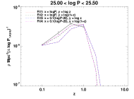
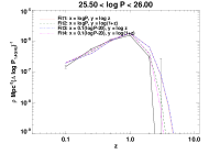
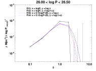
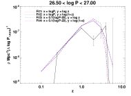
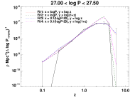
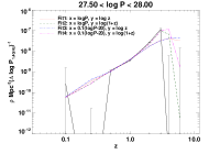
Figure 16: The results of the four smooth fits to the $P$–$z$ grid.

References

- Antonucci (1993) Antonucci R., 1993, ARA&A, 31, 473
- Barthel (1989) Barthel P. D., 1989, ApJ, 336, 606
- Best et al. (1998) Best P. N., Longair M. S., Röttgering H. J. A., 1998, MNRAS, 295, 549
- Best et al. (2003) Best P. N., Arts J. N., Röttgering H. J. A., Rengelink R., Brookes M. H., Wall J., 2003, MNRAS, 346, 627
- Best et al. (2005) Best, P. N., Kauffmann, G., Heckman, T. M., & Ivezić, Ž. 2005, MNRAS, 362, 9
- Best et al. (2011) Best P. N., et al. 2011, in prep
- Best et al. (2003) Best P. N., Peacock J. A., Brookes M. H., Dowsett R. E., Röttgering H. J. A., Dunlop J. S., Lehnert M. D., 2003, MNRAS, 346, 1021
- Best et al. (2006) Best P. N., Kaiser C. R., Heckman T. M., Kauffmann G., 2006, MNRAS, 368, L67
- Best et al. (2007) Best, P. N., von der Linden, A., Kauffmann, G., Heckman, T. M., & Kaiser, C. R. 2007, MNRAS, 379, 894
- Blain et al. (1999) Blain A. W., Smail I., Ivison R. J., Kneib J.-P., 1999, MNRAS, 302, 632
- Bondi et al. (2008) Bondi, M., Ciliegi, P., Schinnerer, E., Smolčić, V., Jahnke, K., Carilli, C., Zamorani, G., 2008, ApJ, 681, 1129
- Boyle et al. (2000) Boyle B. J., Shanks T., Croom S. M., Smith R. J., Miller L., Loaring N., Heymans C., 2000, MNRAS, 317, 1014
- Bower et al. (2006) Bower R. G., Benson A. J., Malbon R., Helly J. C., Frenk C. S., Baugh C. M., Cole S., Lacey C. G., 2006, MNRAS, 370, 645
- Brookes et al. (2006) Brookes M. H., Best P. N., Rengelink R., Röttgering H. J. A., 2006, MNRAS, 366, 1265
- Brookes et al. (2008) Brookes, M. H. and Best, P. N. and Peacock, J. A. and Röttgering, H. J. A. and Dunlop, J. S., 2008, MNRAS, 385, 1297
- Burgess & Hunstead (2006) Burgess, A. M., & Hunstead, R. W. 2006, AJ, 131, 100
- Carilli et al. (1998) Carilli C. L., Menten K. M., Reid M. J., Rupen M. P., Yun M. S., 1998, ApJ, 494, 175
- Colless (1999) Colless M., 1999, Royal Society of London Philosophical Transactions Series A, 357, 105
- Colless et al. (2001) Colless et al. M., 2001, MNRAS, 328, 1039
- Croton et al. (2006) Croton, D. J., et al. 2006, MNRAS, 365, 11
- de Vries et al. (1995) de Vries W. H., Barthel P. D., Hes R., 1995, A&AS, 114, 259
- di Serego-Alighieri et al. (1994) di Serego-Alighieri S., Danziger I. J., Morganti R., Tadhunter C. N., 1994, MNRAS, 269, 998
- Donoso et al. (2009) Donoso, E., Best, P. N. & Kauffmann, G., 2009, MNRAS, 392, 617
- Downes et al. (1986) Downes A. J. B., Peacock J. A., Savage A., Carrie D. R., 1986, MNRAS, 218, 31
- Dunlop & Peacock (1990) Dunlop J. S., Peacock J. A., 1990, MNRAS, 247, 19
- Dunlop & Peacock (1993) Dunlop J. S., Peacock J. A., 1993, MNRAS, 263, 936
- Dunlop et al. (1989) Dunlop J. S., Peacock J. A., Savage A., Lilly S. J., Heasley J. N., Simon A. J. B., 1989, MNRAS, 238, 1171
- Dye & Eales (2010) Dye, S., & Eales, S. 2010, arXiv:1003.3949
- Fabian et al. (2006) Fabian, A. C., Sanders, J. S., Taylor, G. B., Allen, S. W., Crawford, C. S., Johnstone, R. M., & Iwasawa, K. 2006, MNRAS, 366, 417
- Fan (2001) Fan X. et al., 2001, AJ, 121, 54
- Fan (2004) Fan X. et al., 2004, AJ, 128, 515
- Fanaroff & Riley (1974) Fanaroff B.L. and Riley J.M., 1974, MNRAS, 167, 31
- Fanidakis et al. (2010) Fanidakis, N., et al. 2010, arXiv:1011.5222
- Hardcastle et al. (2006) Hardcastle, M. J., Evans, D. A., & Croston, J. H. 2006, MNRAS, 370, 1893
- Hasinger et al. (2005) Hasinger, G., Miyaji, T., & Schmidt, M. 2005, A&A, 441, 417
- Heckman et al. (1994) Heckman T. M., O’Dea C. P., Baum S. A., Laurikainen E., 1994, ApJ, 428, 65
- Huchra et al. (1999) Huchra J. P., Vogeley M. S., Geller M. J., 1999, ApJS, 121, 287
- Grimes et al. (2005) Grimes, J. A., Rawlings, S., & Willott, C. J. 2005, MNRAS, 359, 1345
- Jarvis et al. (2001) Jarvis M. J., Rawlings S., Willott C. J., Blundell K. M., Eales S., Lacy M., 2001, MNRAS, 327, 907
- Jarvis & Rawlings (2000) Jarvis M. J., Rawlings S., 2000, MNRAS, 319, 121
- Jarvis et al. (2009) Jarvis, M. J., Teimourian, H., Simpson, C., Smith, D. J. B., Rawlings, S., & Bonfield, D. 2009, MNRAS, 398, L83
- Jones et al. (2004) Jones, 2004, MNRAS, 355, 747
- Kellermann & Wall (1987) Kellermann, K. I., & Wall, J. V. 1987, Observational Cosmology, 124, 545
- Ker et al. (2011) Ker L. et al. 2011, in prep
- Koo & Kron (1982) Koo D. C., Kron R. G., 1982, A&A, 105, 107
- Kron (1980) Kron R. G., 1980, ApJS, 43, 305
- Labiano et al. (2007) Labiano, A., Barthel, P. D., O’Dea, C. P., de Vries, W. H., Pérez, I. & Baum, S. A., 2007, A&A, 463, 97L
- Laing & Peacock (1980) Laing, R. A., & Peacock, J. A. 1980, MNRAS, 190, 903
- Lawrence et al. (1996) Lawrence C. R., Zucker J. R., Readhead A. C. S., Unwin S. C., Pearson T. J., Xu W., 1996, ApJS, 107, 541
- Mauch et al. (2007) Mauch, 2007, MNRAS, 375, 931
- McCarthy et al. (1996) McCarthy P. J., Kapahi V. K., van Breugel W., Persson S. E., Athreya R., Subrahmanya C. R., 1996, ApJS, 107, 19
- McLure et al. (2006) McLure, R. J., Jarvis, M. J., Targett, T. A., Dunlop, J. S., & Best, P. N. 2006, MNRAS, 368, 1395
- Nelder & Mead (1965) Nelder J. A., Mead R., 1965, Computer Journal, 7, 308
- Osmer (1982) Osmer, P. S. 1982, ApJ, 253, 28
- Owen et al. (1995) Owen F. N., Ledlow M. J., Keel W. C., 1995, AJ, 109, 14
- Peacock & Wall (1981) Peacock, J. A., & Wall, J. V. 1981, MNRAS, 194, 331
- Peacock (1985) Peacock, J. A. 1985, MNRAS, 217, 601
- Perlman et al. (1998) Perlman E. S., Padovani P., Giommi P., Sambruna R., Jones L. R., Tzioumis A., Reynolds J., 1998, AJ, 115, 1253
- Richards et al. (2005) Richards, G. T., et al. 2005, MNRAS, 360, 839
- Rigby, Snellen & Best (2007) Rigby E.E., Snellen I.A.G., Best P.N., 2007, MNRAS, 380, 1449
- Rigby, Snellen & Best (2008) Rigby E.E., Best P.N., Snellen I.A.G., 2008, MNRAS, 385, 310
- Sadler et al. (2002) Sadler, E. M., et al. 2002, MNRAS, 329, 227
- Sandage (1972) Sandage, A. 1972, ApJ, 178, 25
- Schmidt et al. (1988) Schmidt, M., Schneider, D. P., & Gunn, J. E. 1988, Optical Surveys for Quasars, 2, 87
- Seymour et al. (2004) Seymour N., McHardy I. M., Gunn K. F., 2004, MNRAS, 352, 131
- Shaver et al. (1996) Shaver P. A., Wall J. V., Kellermann K. I., Jackson C. A., Hawkins M. R. S., 1996, Nature, 384, 439
- Silverman et al. (2005) Silverman, J. D., et al. 2005, ApJ, 624, 630
- Smolčić et al. (2008) Smolčić, V., et al. 2008, ApJS, 177, 14
- Smolčić et al. (2009) Smolčić V., Schinnerer E., Zamorani G., Bell E. F., Bondi M., Carilli C. L., Ciliegi P., Mobasher B., Paglione T., Scodeggio M., Scoville N., 2009, ApJ, 690, 610
- Snellen et al. (2002) Snellen I. A. G., Lehnert M. D., Bremer M. N., Schilizzi R. T., 2002, MNRAS, 337, 981
- Snellen et al. (2000) Snellen I. A. G., Schilizzi R. T., Miley G. K., de Bruyn A. G., Bremer M. N., Röttgering H. J. A., 2000, MNRAS, 319, 445
- Stickel et al. (1993) Stickel M., Kuehr H., Fried J. W., 1993, A&AS, 97, 483
- Tadhunter et al. (2001) Tadhunter C., Wills K., Morganti R., Oosterloo T., Dickson R., 2001, MNRAS, 327, 227
- Tadhunter et al. (1993) Tadhunter C. N., Morganti R., di Serego-Alighieri S., Fosbury R. A. E., Danziger I. J., 1993, MNRAS, 263, 999
- The NED Team (1992) The NED Team, 1992
- Ueda et al. (2003) Ueda, Y., Akiyama, M., Ohta, K., & Miyaji, T. 2003, ApJ, 598, 886
- Ubachukwu et al. (1996) Ubachukwu, A. A., Ugwoke, A. C., & Ogwo, J. N., 1996, Ap&SS, 238, 151U
- Vestergaard & Osmer (2009) Vestergaard, M., & Osmer, P. S. 2009, ApJ, 699, 800
- Waddington (1999) Waddington I., 1999, PhD thesis, University of Edinburgh
- Waddington et al. (2001) Waddington I., Dunlop J. S., Peacock J. A., Windhorst R. A., 2001, MNRAS, 328, 882
- Waddington et al. (2000) Waddington I., Windhorst R. A., Dunlop J. S., Koo D. C., Peacock J. A., 2000, MNRAS, 317, 801
- Wall (2008) Wall, J. 2008, arXiv:0807.3792
- Wall et al. (2005) Wall J. V., Jackson C. A., Shaver P. A., Hook I. M., Kellermann K. I., 2005, A&A, 434, 133
- Wall & Peacock (1999) Wall J. V., Peacock J. A., 1999, VizieR Online Data Catalog, 721, 60173
- Wall & Peacock (1985) Wall J. V., Peacock J. A., 1985, MNRAS, 216, 173
- Wall et al. (1968) Wall, J. V., Cole, D. J., & Milne, D. K. 1968, Proceedings of the Astronomical Society of Australia, 1, 98
- White et al. (1997) White R. L., Becker R. H., Helfand D. J., Gregg M. D., 1997, ApJ, 475, 479
- Willott et al. (2003) Willott C. J., Rawlings S., Jarvis M. J., Blundell K. M., 2003, MNRAS, 339, 173
- Willott et al. (2001) Willott, C. J., Rawlings, S., Blundell, K. M., Lacy, M., & Eales, S. A. 2001, MNRAS, 322, 536
- Wilman et al. (2008) Wilman, R. J., et al. 2008, MNRAS, 388, 1335
- Windhorst et al. (1984) Windhorst R. A., Kron R. G., Koo D. C., 1984, A&AS, 58, 39
- Windhorst et al. (1984) Windhorst R. A., van Heerde G. M., Katgert P., 1984, A&AS, 58, 1
- York et al. (2000) York D. G., Adelman J., Anderson J. E., et al. AJ, 120, 1579
- Wolf et al. (2003) Wolf C., Wisotzki L., Borch A., Dye S., Kleinheinrich M., Meisenheimer K., 2003, A&A, 408, 499
- De Zotti et al. (2010) De Zotti, G., Massardi, M., Negrello, M., & Wall, J. 2010, A&A Rev., 18, 1