The ‘Butterfly effect’ in Cayley graphs, and its relevance for evolutionary genomics

Abstract

Suppose a finite set $X$ is repeatedly transformed by a sequence of permutations of a certain type acting on an initial element $x$ to produce a final state $y$. We investigate how ‘different’ the resulting state $y^{\prime}$ to $y$ can be if a slight change is made to the sequence, either by deleting one permutation, or replacing it with another. Here the ‘difference’ between $y$ and $y^{\prime}$ might be measured by the minimum number of permutations of the permitted type required to transform $y$ to $y^{\prime}$, or by some other metric. We discuss this first in the general setting of sensitivity to perturbation of walks in Cayley graphs of groups with a specified set of generators. We then investigate some permutation groups and generators arising in computational genomics, and the statistical implications of the findings.

1 Introduction

In evolutionary genomics, two genomes are frequently compared by the minimum number of ‘rearrangements’ (of various types) required to transform one genome into another [7]. This minimum number is then used to estimate of the actual number of events and thereby the ‘evolutionary distance’ between the species involved. Since both the precise number and the actual rearrangement events that occurred in the evolution of the two genomes from a common ancestor are unknown, it is pertinent to have some idea of how sensitive this distance estimate might be to the sequence of events (not just the number) that really took place [19].

This question has important implications for the accurate inference of evolutionary relationships between species from their genomes, and we discuss some of these further in Section 5. However, we begin by framing the type of mathematical questions that we will be considering in a general algebraic context.

Let $G$ be a finite group, whose identity element we write as $1_{G}$, and let $S$ be a subset of generators, that is symmetric (i.e. closed under inverses, so $x\in S\Rightarrow x^{-1}\in S$). In addition, let $\Gamma=Cay(G,S)$ be the associated Cayley graph, with vertex set $G$ and an edge connecting $g$ and $g^{\prime}$ if there exists $s\in S$ with $g^{\prime}=gs$ (unless otherwise stated, we use the convention of multiplying group elements from left to right). For any two elements $g,g^{\prime}\in G$, the distance $d_{S}(g,g^{\prime})$ in $Cay(G,S)$ is the minimum value of $k$ for which there exist elements $s_{1},\ldots,s_{k}$ of $S$ so that $g^{\prime}=gs_{1}\cdots s_{k}$ (for $g=g^{\prime}$, we set $d_{S}(g,g^{\prime})=0$). Note that $d_{S}$ is a metric, in particular, $d_{S}(g,g^{\prime})=d_{S}(g^{\prime},g)$, since $S$ is symmetric.

In this paper, our focus is on the following two quantities:

$$\lambda_{1}(G,S):=\mathop{\displaystyle\max}_{\scriptscriptstyle g\in G,s\in S}\limits\{d_{S}(sg,g)\},$$

and

$$\lambda_{2}(G,S):=\mathop{\displaystyle\max}_{\scriptscriptstyle g\in G,s,s^{\prime}\in S}\limits\{d_{S}(sg,s^{\prime}g)\}.$$

One way to view these quantities is via the following result which is easily proved.

Lemma 1

Let $S$ be a symmetric set of generators for a finite group $G$. Then:

• $\lambda_{1}(G,S)$ is the maximum value of $d_{S}(g,g^{\prime})$ between any pair of elements $g$ and $g^{\prime}$ of $G$ for which $g=s_{1}s_{2}\cdots s_{k}$, and $g^{\prime}=s^{\prime}_{1}s^{\prime}_{2}\cdots s^{\prime}_{k}$, where $s^{\prime}_{i}=s_{i}\in S$ for all but at most one value (say $j$) for $i$, and $s^{\prime}_{j}=1_{G}$.

• $\lambda_{2}(G,S)$ is the maximum value of $d_{S}(g,g^{\prime})$ between any pair of elements $g$ and $g^{\prime}$ of $G$ for which $g=s_{1}s_{2}\cdots s_{k}$ and $g^{\prime}=s^{\prime}_{1}s^{\prime}_{2}\cdots s^{\prime}_{k}$ where $s^{\prime}_{i}=s_{i}\in S$ for all but at most one value (say $j$) for $i$, and $s^{\prime}_{j}\in S,s^{\prime}_{j}\neq s_{j}$.

Thus, $\lambda_{1}(G,S)$ tells us how much (under $d_{S}$) a product of generators can change if we drop one value of $s$, whilst $\lambda_{2}(G,S)$ tells us how much (again under $d_{S}$) a product of generators in $S$ can change if we substitute one value of $s$ by another $s^{\prime}$ (see Fig. 1 for an example where $\lambda_{2}(G,S)=6$).

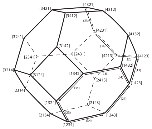
Figure 1: The Cayley graph $Cay(G,S)$ for $G=\Sigma_{4}$ (the permutation group on $\{1,2,3,4\}$) and the set of transpositions $S=\{(12),(23),(34)\}$. Substituting just one element – namely (34) for (12) – in the product corresponding to the walk in the lower front face (which starts and returns to the lower-most point [1234]) results in a walk that ends at a point ([4321], top) that is very distant (under $d_{S}$) from the end-point of the original walk. In fact, the two end-points are at maximal distance in this example.

As such, $\lambda_{m}$ is a measure of the ‘sensitivity’ of walks in the Cayley graph to a switch in or deletion of a generator at some point. Moreover, if $G$ acts transitively and freely on a set $X$ then $\lambda_{m}$ provides a corresponding measure of sensitivity of this action to a switch in or deletion of a generator (since a transitive, free action of $G$ on $X$ is isomorphic to the action of $G$ on itself by right multiplication). Actions with large $\lambda_{m}$ values can thus be viewed as exhibiting a discrete, group-theoretic analogue of the ‘butterfly effect’ in non-linear dynamics (see e.g. [9]).

In the genomics applications that we shall consider, elements of the group $G$ correspond to genomes, and $d_{S}$ to the evolutionary distance between them. After presenting some general results concerning $\lambda_{m}$ in the next section, in Sections 3 and 4 we discuss some applications arising for various choices of $G$ and $S$. These include the Klein four group, which arises in evolutionary models of DNA sequence evolution, and the permutatation group, which typically appears when studying rearrangement distances between genomes. We conclude in Section 5 with some statistical implications of our results.

One can imagine many other settings besides genomics where similar questions arise – for example, in a sequence of moves that should unscramble the Rubik’s cube from a given position [12], what will be the consequences (in terms of the number of moves required) for completing the unscrambling if a mistake is made at some point (or one move is forgotten)? In addition, related questions arise in the study of ‘automatic’ groups, where the group under consideration is typically infinite [4].

2 General inequalities

We first make some basic observations about Cayley graphs and the metric $d_{S}$ (further background on basic group theory, Cayley graphs, and group actions can be found in [15]). It is well known that $\Gamma$ is a connected regular graph of degree equal to the cardinality of $S$ and that $\Gamma$ is also vertex-transitive (see, for example, [11], Proposition 1). Consider the function $l_{S}:G\rightarrow\{0,1,2,3\ldots|G|\}$, where, $l_{S}(1_{G})=0$ and, for each $g\in G-\{1_{G}\}$, $l_{S}(g)$ is the smallest number $l$ of elements $s_{1},\ldots,s_{l}$ from $S$ for which we can write $g=s_{1}\cdots s_{l}.$ The function $l_{S}$ clearly satisfies the subadditivity property that, for all $g,g^{\prime}\in G$:

$$l_{S}(gg^{\prime})\leq l_{S}(g)+l_{S}(g^{\prime}).$$

In addition,

$$l_{S}(g^{-1})=l_{S}(g),$$

and

$$l_{S}(g)=1\Leftrightarrow g\in S,l_{S}(g)=0\Leftrightarrow g=1_{G}.$$

Note that $l_{S}(gg^{\prime})$ is generally not equal to $l_{S}(g^{\prime}g)$. The metric $d_{S}$, described in the previous section, is related to $l_{S}$ as follows:

$$d_{S}(g,g^{\prime})=l_{S}(g^{-1}g^{\prime}).$$

Consequently, by definition:

$$\lambda_{1}(G,S)=\mathop{\displaystyle\max}_{\scriptscriptstyle g\in G,s\in S}\limits\{l_{S}(g^{-1}sg)\},$$ (1)

and

$$\lambda_{2}(G,S)=\mathop{\displaystyle\max}_{\scriptscriptstyle g\in G,s,s^{\prime}\in S}\limits\{l_{S}(g^{-1}ss^{\prime}g)\}.$$ (2)

Let $l_{S}(G)=\max\{l_{S}(g):g\in G\}$, which is the diameter of $Cay(G,S)$, that is, maximum length shortest path connecting any two elements of $G$. Clearly, $\lambda_{1}(G,S),\lambda_{2}(G,S)\leq l_{S}(G)$. Moreover:

$$\lambda_{2}(G,S)\leq 2\cdot\lambda_{1}(G,S),$$ (3)

since, for any $g\in G$ and $s,s^{\prime}\in S$, we have:

$$d_{S}(sg,s^{\prime}g)\leq d_{S}(sg,g)+d_{S}(g,s^{\prime}g).$$

A partial converse to Inequality (3) is provided by the following:

$$\lambda_{1}(G,S)\leq\lambda_{2}(G,S)+\lambda^{\prime}_{1}(G,S),$$ (4)

where $\lambda^{\prime}_{1}(G,S)=\max_{g\in G}\min_{s\in S}\{l_{S}(g^{-1}sg)\}.$ To verify (4), select a pair $g\in G,s\in S$ so that $l_{S}(g^{-1}sg)=\lambda_{1}(G,S).$ Then:

$$\lambda_{1}(G,S)=d_{S}(sg,g)\leq d_{S}(sg,s_{1}g)+d_{S}(s_{1}g,g),$$

where $s_{1}$ is an element $s^{\prime}$ (possibly equal to $s$) in $S$ that minimizes $l_{S}(g^{-1}s^{\prime}g)$. Now, $d_{S}(sg,s_{1}g)\leq\lambda_{2}(G,S)$ (even if $s^{\prime}=s$) and $d_{S}(s_{1}g,g)\leq\lambda^{\prime}_{1}(G,S)$, and so we obtain (4).

Note also that if $G$ is Abelian, then $\lambda_{1}(G,S)=1$, and $\lambda_{2}(G,S)\leq 2$ for any symmetric set $S$ of generators. Moreover, for the Abelian 2-group $G={\mathbb{Z}}_{2}^{n}$ and with the symmetric set $S$ of generators consisting of all $n$ elements with the identity at all but one position, we have $l_{S}(G)=n$ and $\lambda_{1}(G,S)=1$. This shows that the inequality $\lambda_{1}(G,S)\leq l_{S}(G)$ can be arbitrarily large. Our next result generalizes this observation further.

Lemma 2

Let $G_{1},G_{2},\ldots,G_{k}$ be finite groups, and let $S_{i}$ be a symmetric set of generators of $G_{i}$ for $i=1,\ldots,n$. Consider the direct product $G=G_{1}\times G_{2}\times\cdots\times G_{k}$ along with the symmetric set of generators $S$ of $G$ consisting of all possible $k$–tuples which consist of the identity element of $G_{i}$ at all but one co-ordinate $i$, where it takes some value in $S_{i}$. Then (i) $\lambda_{1}(G,S)\leq\max_{1\leq i\leq k}\big{\{}l_{S_{i}}(G_{i})\big{\}},$ and (ii) $l_{S}(G)=\sum_{i=1}^{k}l_{S_{i}}(G_{i}).$

Proof: For Part (i), let $\lambda_{1}(G,S)=l_{S}(g^{-1}sg)$, where $s\in S$ is a non-identity element at some co-ordinate $\nu$. Notice that $(g^{-1}sg)_{j}=1_{G_{j}}$ for all $j\neq\nu$. Moreover, $(g^{-1}sg)_{\nu}=s_{1}\cdots s_{l}$ where $l\leq l_{S_{\nu}}(G_{\nu})$. Thus $l_{S}(g^{-1}sg)\leq l_{S_{\nu}}(G_{\nu})$, as claimed.

For Part (ii), the inequality $l_{S}(G)\leq\sum_{i=1}^{k}l_{S_{i}}(G_{i})$ is clear; to establish the reverse inequality, let $g_{i}$ be an element of $G_{i}$ with $l_{S_{i}}(g_{i})=l_{S_{i}}(G_{i})$, and $g=(g_{1},\ldots,g_{k})\in G$. Then $l_{S}(g)=\sum_{i=1}^{k}l_{S_{i}}(G_{i}),$ and so $l_{S}(G)\geq\sum_{i=1}^{k}l_{S_{i}}(G_{i}).$ $\Box$

We now consider how $\lambda_{m}$ behaves under group homomorphisms. Suppose $H$ is the homomorphic image of a group $G$ under a map $p$. Let $N=Ker(p)$ be the kernel of $p$, which is a normal subgroup of $G$, and with $H\cong G/N$. Thus we have a short exact sequence:

$$1\rightarrow N\rightarrow G\buildrel p\over{\rightarrow}H\rightarrow 1.$$ (5)

Let $S$ be a symmetric set of generators of $G$. Then $S_{H}=\{p(s):s\in S-N\}$ is a symmetric set of generators of $H$.

Lemma 3

For $m=1,2$, $\lambda_{m}(H,S_{H})\leq\lambda_{m}(G,S).$

Proof: First suppose that $m=1$. For $x\in S_{H}$ and $h\in H$, consider $h^{-1}xh$. There exist elements $g\in G$ and $s\in S-N$ for which $f(g)=h$ and $f(s)=x$. Now the element $g^{-1}sg\in G$ can be written as a product of at most $l=\lambda_{1}(G,S)$ elements of $S$, that is $g^{-1}sg=s_{1}s_{2}\cdots s_{k}$ for $k\leq l$. Applying $p$ to both sides of this equation gives: $h^{-1}xh=p(s_{1})p(s_{2})\cdots p(s_{k})$. Notice that some of the elements on right may equal the identity element of $H$ (since $p(s_{i})=1_{H}\Leftrightarrow s_{i}\in N$), but they are elements of $S_{H}$ otherwise. Thus $l_{S_{H}}(h^{-1}xh)\leq l$. Since this holds for all such elements $h,x$, Eqn. (1) shows that $\lambda_{1}(H,S_{H})\leq\lambda_{1}(G,S)$. The corresponding result for $m=2$ follows by an analogous argument. $\Box$

To obtain a lower bound for $\lambda_{m}(G,S)$ suppose that the short exact sequence (5) is a split extension, i.e. there is a homomorphism $i:H\rightarrow G$ so that $p\circ i$ is the identity map on $H$, which (by the splitting lemma) is equivalent to the condition that $G$ is the semidirect product of $N$ with a subgroup $H^{\prime}$ isomorphic to $H$ (i.e. $G=NH^{\prime}=H^{\prime}N,H^{\prime}\cap N=\{1_{G}\}$). In this case we have the following bounds.

Proposition 4

Suppose a finite group $G$ is a semidirect product of subgroups $N$ (normal) and $H$. Let $S_{N},S_{H}$ be symmetric generator sets for $N$ and $H$ respectively, and let $S=S_{N}\cup S_{H}$ which is a symmetric generator set for $G$. Then:

$$\lambda_{1}(H,S_{H})\leq\lambda_{1}(G,S)\leq\lambda_{1}(H,S_{H})+l_{S_{N}}(N).$$

In particular, by (3), $\lambda_{2}(G,S)\leq 2\lambda_{1}(H,S_{H})+2l_{S_{N}}(N).$

Proof: The lower bound on $\lambda_{1}(G,S)$ follows from Lemma 3. For the upper bound we must show that for all $s\in S$ and $g\in G$, $d_{S}(sg,g)\leq\lambda_{1}(H,S_{H})+l_{S_{N}}(N)$ holds. We consider two cases: (i) $s\in N$, and (ii) $s\in H$. In Case (i), note that the conjugate element $g^{-1}sg$ is also an element of $N$; in this case we have the tighter bound $d_{S}(sg,g)\leq l_{S_{N}}(N)$. In Case (ii), write $g=hn$ where $n\in N$ and $h\in H$. Consider the word

$$w=g^{-1}sg=n^{-1}h^{-1}shn.$$

Since $N$ is normal we have $n^{-1}(h^{-1}sh)=(h^{-1}sh)n^{\prime}$ for some element $n^{\prime}\in N$. Thus $w=h^{-1}shn^{\prime}n.$ Write $w=w_{1}w_{2}$ where $w_{1}=h^{-1}sh\in H$ and $w_{2}=n^{\prime}n\in N$. We can select $w_{2}$ to be a product of terms of $S_{N}$ of length at most $l_{S_{N}}(N)$ and, by Inequality (3), we can select $w_{1}$ to be a product of terms of $S_{H}$ of length at most $\lambda_{1}(H,S_{H})$. Thus $w$ can be written as a product of, at most, $\lambda_{1}(H,S_{H})+l_{S_{N}}(N)$ elements of $S$. $\Box$

3 Permutation groups and genomic applications

We first describe a direct application that is relevant to the evolution of a DNA sequence under a simple model of site substitution (Kimura’s 3ST model) [10]. Consider the four-letter DNA alphabet ${\mathcal{A}}=\{A,C,G,T\}$ and the Klein four-group $K={\mathbb{Z}}_{2}\times{\mathbb{Z}}_{2}$ with an action on ${\mathcal{A}}$ in which the three non-zero elements of $K$ correspond to ‘transitions’ (A $\leftrightarrow$ G, C $\leftrightarrow$ T) and the two types of ‘transversions’ (A$\leftrightarrow$C, G$\leftrightarrow$T; and A$\leftrightarrow$T, G$\leftrightarrow$C). This representation of the Kimura 3ST model was first described and exploited by [6].

For $g\in K$ and $x\in{\mathcal{A}}$, let $g\circ x$ denote the element of ${\mathcal{A}}$ obtained by the action of $g$ on $x$ (the identity element fixes each element of ${\mathcal{A}}$). The resulting component-wise action of $K^{n}$ on ${\mathcal{A}}^{n}$, defined by: $(g_{1},\ldots g_{n})\circ(x_{1},\ldots x_{n})=(g_{1}\circ x_{1},\ldots,g_{n}\circ x_{n})$, can be regarded as the set of all changes that can occur to a DNA sequence over a period of time under site substitutions.

Now, under any continuous-time Markovian process these change events (‘site substitutions’) occur just one at a time and so a natural generating set of $K^{n}$ is the set $S_{n}$ of all elements of $K^{n}$ that consist of $1_{K}$ at all but one co-ordinate. Moreover, since the action of $K^{n}$ on ${\mathcal{A}}^{n}$ is transitive and free (and so is isomorphic to the action of $K^{n}$ on itself by right multiplication), $\lambda_{m}(K^{n},S_{n})$ measures the impact of ignoring (for $m=1$) or replacing (for $m=2$) one substitution in a chain of such events over time. As $K^{n}$ is Abelian, one has $\lambda_{1}(K^{n},S_{n})=1$ and $\lambda_{2}(K^{n},S_{n})=2$, which implies that this impact is minor, and, more significantly, is independent of $n$; this has important statistical implications which we will describe further in Section 5.

For a related example, consider the ordered sequence of distinct genes $(g_{1},g_{2},\ldots,g_{n})$ partitioned into regions $R_{1},R_{2},\ldots R_{k}$ so that genomic rearrangements occur within each region, but not between regions (e.g. $R_{i}$ might refer to different chromosomes). This situation can be modelled by the setting of Lemma 2 in which $G_{i}$ is a permutation group on the genes within $R_{i}$, and $S_{i}$ is set of elementary gene order rearrangement events that generates $G_{i}$ (we discuss some examples below). In this case, Lemma 2 provides a bound on $\lambda_{1}$ and $\lambda_{2}$ that is independent of the number of regions $k$.

We turn now to the calculation of $\lambda_{m}(\Sigma_{n},S)$ for the permutation group $\Sigma_{n}$ on $n!$ elements and various sets $S$ of generators. This group commonly arises when studying genome rearrangements [11]. Our main interest is to determine, for each instance of $S$, whether there is a constant $C$ (independent of $n$) for which $\lambda_{m}(\Sigma_{n},S)\leq C$, for $m=1,2$.

A permutation $g$ on the set $[n]:=\{1,2,\dots,n\}$ is a bijective mapping from $[n]$ to itself. We will also write $g$ as $g=[g_{1},g_{2},\dots,g_{n}]$ where $g_{i}=g(i)$ is the image of the map $g$ for $i\in[n]$. Note that, following the usual convention, the product $gg^{\prime}$ of two permutations $g,g^{\prime}\in\Sigma_{n}$ will be considered as the composition of the functions $g$ and $g^{\prime}$. In particular, $gg^{\prime}(i)=g(g^{\prime}(i))$ for all $i\in[n]$.

When studying genomes, each entry $g_{i}$ of a permutation $g$ corresponds to a gene and the full list $[g_{1},g_{2},\dots,g_{n}]$ to a genome. Multiplying $g$ by a permutation leads to a rearrangement of the genome. For example, multiplying by a transposition $t_{i,j}$ interchanges the values at positions $i$ and $j$ of $g$, i.e. $[\dots,g_{i},\dots,g_{j},\dots]t_{i,j}=[\dots,g_{j},\dots,g_{i},\dots]$, and multiplying by a reversal $r_{i,j}$ reverses the segment $[g_{i},g_{j}]$, $1\leq i<j\leq n$, of $g$, i.e.

$$[\dots,g_{i},g_{i+1},\dots,g_{j-1},g_{j},\dots]r_{i,j}=[\dots,g_{j},g_{j-1},\dots,g_{i+1},g_{i},\dots].$$

Such rearrangements are widely observed and studied in molecular biology [7].

In genomics applications, we are often interested in defining some distance between genomes. One distance that is commonly used in the context of permutations is the breakpoint distance [17, 7.3]. For $g,g^{\prime}\in\Sigma_{n}$, $d_{BP}(g,g^{\prime})$ is defined as the number of pairs of elements that are adjacent in the list $[0,g_{1},g_{2},\dots,g_{n},n+1]$, but not in the list $[0,g^{\prime}_{1},g^{\prime}_{2},\dots,g^{\prime}_{n},n+1]$. For example, if $g=[1,2,3,4,5],g^{\prime}=[1,4,3,2,5]\in\Sigma_{5}$, we have $d_{BP}(g,g^{\prime})=2$. It is clear that $\max\{d_{BP}(g,g)\,:\,g,g^{\prime}\in\Sigma_{n}\}=n+1$.

Alternatively, one can consider the rearrangment distance between two genomes, i.e. the minimal number of operations of a certain type (such as transpositions or reversals) that can be applied to one of the genomes to obtain the other [7]. In terms of Cayley graphs, this distance can be conveniently expressed for transpositions and reversals as follows. Let

$$T=T_{n}:=\{t_{i,j}\in\Sigma_{n}\,:\,1\leq i<j\leq n\},$$

$$C=C_{n}:=\{t_{i,i+1}\in T\,:\,1\leq i\leq n-1\},$$

(the Coxeter generators), and

$$R:=\{r_{i,j}\in\Sigma_{n}\,:\,1\leq i<j\leq n\}.$$

Note that all three of these sets generate $\Sigma_{n}$ [11] and that they are all symmetric, since each generator is its own inverse. The metric $d_{S}$, $S=T,C,R$, is precisely the rearrangement distance.

The diameters of $Cay(\Sigma_{n},T)$ and $Cay(\Sigma_{n},R)$ are both $n-1$, and the diameter of $Cay(\Sigma_{n},C)$ is ${n\choose 2}$ [11].

Regarding the quantities $\lambda_{m}(\Sigma_{n},S)$, we have the following result for $S=T,C,R$:

Theorem 5

For $n\geq 7$ the following hold:

• $\lambda_{1}(\Sigma_{n},T_{n})=1$ and $\lambda_{2}(\Sigma_{n},T_{n})=2$.

• $\lambda_{1}(\Sigma_{n},C_{n})=2n-3$ and $2n-2\leq\lambda_{2}(\Sigma_{n},C_{n})\leq 4n-6$.

• $\frac{n+1}{2}\leq\lambda_{m}(\Sigma_{n},R_{n})\leq n-1$, $m=1,2$.

Proof: (i) Note that if $g\in\Sigma_{n}$ and $t_{i,j}\in T$, then:

$$g^{-1}t_{i,j}g=t_{g^{-1}(i),g^{-1}(j)}.$$ (6)

Therefore $\lambda_{1}(\Sigma_{n},T)=1$ by (1). Thus, by Inequality (3), we have $\lambda_{2}(\Sigma_{n},T)\leq 2$. The equality $\lambda_{2}(\Sigma_{n},T)=2$ follows by (2) and the fact that $g^{-1}t_{k,l}t_{i,j}g=t_{g^{-1}(i),g^{-1}(j)}t_{g^{-1}(k),g^{-1}(l)}$ holds for any $g\in\Sigma_{n}$ and $1\leq i<j<k<l\leq n$.

(ii) Consider the permutation $g\in\Sigma_{n}$ given by $g=[2,3,\dots,n-1,n,1]$. Then $g^{-1}t_{1,2}g=[n,2,3,\dots,n-1,1]$. Therefore, $l_{C}(g^{-1}t_{1,2}g)\geq 2n-3$ (since to transform $[n,2,3,\dots,n-1,1]$ to $1_{\Sigma_{n}}$ requires moving $1$ and $n$ back to their original positions). Therefore, $\lambda_{1}(\Sigma_{n},C)\geq 2n-3$ by (1). But, by Equality (6), $\lambda_{1}(\Sigma_{n},C)\leq 2n-3$, since any transposition is the product of at most $2n-3$ elements in $C$. In particular, $\lambda_{1}(\Sigma_{n},C)=2n-3$.

Similarly, $l_{C}(g^{-1}t_{1,2}t_{3,4}g)\geq 2n-2$, and so $\lambda_{2}(\Sigma_{n},C)\geq 2n-2$ by (2). Hence, by Inequality (3), we have $\lambda_{2}(\Sigma_{n},C)\leq 2(2n-3)$.

(iii) The inequality $\lambda_{m}(\Sigma_{n},R_{n})\leq n-1$, $m=1,2$ follows as the diameter of $Cay(\Sigma_{n},R)$ is at most $n-1$.

Now, suppose $n$ is odd. Let $g\in\Sigma_{n}$ be given by $g=[3,2,5,4,7,6,\dots,n-3,n,n-1,1]$. Then it is straight-forward to check that $d_{BP}(r_{1,n}g,g)=n+1$ (see Figure 2 for the case $n=7$). In particular, since the length of any shortest path in $Cay(\Sigma_{n},R)$ joining any $g,h\in\Sigma_{n}$ is at least $d_{BP}(h,g)/2$ by [17, p.238], we have $\lambda_{1}(\Sigma_{n},R)\geq\frac{n+1}{2}$. Similarly, $d_{BP}(r_{2,3}r_{1,n}g,g)=n+1$ for any $g\in\Sigma_{n}$, and so $\lambda_{2}(\Sigma_{n},R)\geq\frac{n+1}{2}$.

Figure 2: (a) A diagrammatic respresentation of the element $g=[3,2,5,4,6,7,1]$ in $\Sigma_{7}$, defined in the proof of Theorem 5 (iii). (b) The product $r_{1,7}g=[5,6,3,4,1,2,7]$. Note that $d_{BP}(r_{1,7}g,g)=8$.

In case $n$ is even, consider $g=[3,2,5,4,7,6,\dots,n-4,n-1,n-2,1,n]$. Then $d_{BP}(r_{2,n}g,g)=n+1$ and $d_{BP}(r_{3,4}r_{2,n}g,g)=n+1$. Similar reasoning yields the desired result. $\Box$

In genomics, the direction in which a gene is oriented in a genome can also provide useful information to incorporate in rearrangement models, which can be expressed as follows in terms of Cayley graphs [11]. The hyperoctahedral group $B_{n}$ is defined as the group of all permutations $g^{\sigma}$ acting on the set $\{\pm 1,\dots,\pm n\}$ such that $g^{\sigma}(-i)=-g^{\sigma}(i)$ for all $i\in[n]$. An element of $B_{n}$ is a signed permutation. Signed versions of transpositions and reversals can be defined in the obvious way; a sign change transposition $t^{\sigma}_{i,j}$ switches the values in the $i$th and $j$th positions of a signed permutation as well as both of their signs and so forth. Note that we also allow $i=j$ for signed transpositions and reversals so that $t_{i,i}=r_{i,i}$, $i\in[n]$, simply switches the sign of the $i$th value. We denote the set of signed elements corresponding to those in $S=T,C,R$, together with the elements $t_{i,i},1\leq i\leq n$, by $S^{\sigma}$. Note that the diameter of $Cay(B_{n},R^{\sigma})$ is $n+1$ [11].

Now, regarding the group $B_{n}$ as a wreath product [11, p. 2756], we have a short exact sequence:

$$1\rightarrow N\rightarrow B_{n}\buildrel p\over{\rightarrow}\Sigma_{n}\rightarrow 1,$$ (7)

where the homomorphism $p:B_{n}\rightarrow\Sigma_{n}$ sends $g^{\sigma}\in B_{n}$ to the permutation of $[n]$ that maps $i$ to $|g^{\sigma}(i)|$ (i.e. it ignores the sign). Notice that $p$ maps $S^{\sigma}$ onto $S$ when $S=T,C,R$. In particular, from Lemma 3, the following holds for $m=1,2$:

$$\lambda_{m}(B_{n},S^{\sigma})\geq\lambda_{m}(\Sigma_{n},S).$$ (8)

Moreover, $N=Ker(p)$ is isomorphic to the elementary Abelian 2-group ${\mathbb{Z}}_{2}^{n}$ and the short exact sequence in (7) splits, so $B_{n}$ is a semidirect product of ${\mathbb{Z}}_{2}^{n}$ and a subgroup isomorphic to $\Sigma_{n}$. Using these observations, we obtain:

Corollary 6

For $n\geq 7$, the following hold:

• $\lambda_{1}(B_{n},T_{n}^{\sigma})\leq 3$ and $\lambda_{2}(B_{n},T_{n}^{\sigma})\leq 6$.

• $2n-3\leq\lambda_{1}(B_{n},C_{n}^{\sigma})\leq 2n-1$ and $2n-2\leq\lambda_{2}(B_{n},C_{n}^{\sigma})\leq 4n-2$.

• $\frac{n+1}{2}\leq\lambda_{m}(B_{n},R_{n}^{\sigma})\leq n+1$, $m=1,2$.

Proof: The inequalities $\lambda_{1}(B_{n},T_{n}^{\sigma})\leq 3$ and $\lambda_{1}(B_{n},C_{n}^{\sigma})\leq 2n-1$ follow from similar arguments to those used in the proof of Theorem 5 (i) and (ii), using the signed analogue of Equation (6). Inequality (3) then implies that inequalities $\lambda_{2}(B_{n},T_{n}^{\sigma})\leq 6$ and $\lambda_{2}(B_{n},C_{n}^{\sigma})\leq 4n-2$ both hold. The inequality $\lambda_{m}(B_{n},R^{\sigma}_{n})\leq n+1$, $m=1,2$, follows as the diameter of $Cay(B_{n},R^{\sigma}_{n})$ is at most $n+1$. The inequalities $2n-3\leq\lambda_{1}(B_{n},C_{n}^{\sigma})$ and $2n-2\leq\lambda_{2}(B_{n},C_{n}^{\sigma})$, and the remaining ones in (iii) follow by Inequality (8) and Theorem 5. $\Box$

4 Beyond $d_{S}$: properties of breakpoint distance

As we have seen for the breakpoint distance on $\Sigma_{n}$ in the last section, it can sometimes be useful to consider metrics on a group other than the distance $d_{S}$ arising from some Cayley graph. Motivated by this, given an arbitrary metric $d$ on a finite group $G$, with symmetric generator set $S$, we define:

$$\lambda_{1}(G,S,d):=\mathop{\displaystyle\max}_{\scriptscriptstyle g\in G,s\in S}\limits\{d(sg,g)\}\mbox{ and }\lambda_{2}(G,S,d):=\mathop{\displaystyle\max}_{\scriptscriptstyle g\in G,s,s^{\prime}\in S}\limits\{d(sg,s^{\prime}g)\}.$$

In particular, $\lambda_{m}(G,S)=\lambda_{m}(G,S,d_{S})$ and $\lambda_{m}(G,S,d)\leq\max_{g,g^{\prime}\in G}\{d(g,g^{\prime})\}$, $m=1,2$. Moreover, the following analogue of Inequality (3) for an arbitrary metric $d$ on $G$ is easily seen to hold:

$$\lambda_{2}(G,S,d)\leq 2\cdot\lambda_{1}(G,S,d).$$ (9)

Note that, although the quantities $\lambda_{m}(G,S)$ and $\lambda_{m}(G,S,d)$ need not be directly related to one another, in certain circumstances, they are. For example, if $d$ has the property that $d(g,gs)\leq c$ for some constant $c$ it is an easy exercise to show that $\lambda_{m}(G,S,d)\leq c\cdot\lambda_{m}(G,S),$ for $m=1,2$.

We now return to considering the breakpoint distance $d_{BP}$. In genomics, this distance is commonly used as a proxy for rearrangement distances. Thus it is of interest to note:

Lemma 7

For $n\geq 7$, the following hold:

• $\lambda_{1}(\Sigma_{n},T_{n},d_{BP})\leq 4$ and $\lambda_{2}(\Sigma_{n},T_{n},d_{BP})\leq 8$.

• $\lambda_{1}(\Sigma_{n},C_{n},d_{BP})\leq 4$ and $\lambda_{2}(\Sigma_{n},C_{n},d_{BP})\leq 8$.

• $\frac{n+1}{2}\leq\lambda_{m}(\Sigma_{n},R_{n},d_{BP})\leq n+1$, $m=1,2$.

Proof: Suppose $t=t_{i,j}\in T_{n}$, $1\leq i<j\leq n$. Using Equation (6), it is straightforward to see that $d_{BP}(tg,g)\leq 4$ holds for any $g\in\Sigma_{n}$. Therefore $\lambda_{1}(\Sigma_{n},T_{n},d_{BP}),\lambda_{1}(\Sigma_{n},C_{n},d_{BP})\leq 4$. The inequalities in (i) and (ii) involving $\lambda_{2}$ now follow from Inequality (9).

The Inequalities in (iii) follow from the argument used in the proof of Theorem 5 (iii) and the diameter of $d_{BP}$ on $\Sigma_{n}$. $\Box$

In particular, for $C$, the set of Coxeter generators of $\Sigma_{n}$ in the last section, and $m=1,2$, we have $\lambda_{m}(\Sigma_{n},C)\geq 2n-3$, but $\lambda_{m}(\Sigma_{n},C,d_{BP})\leq 4$. Intriguingly, this observation can be extended as follows. For $k\geq 1$, let $R^{(k)}$, denote the set of reversals of the form $\{r_{i,j}\,:\,1\leq i<j\leq n,|i-j|\leq k\}$. Such ‘fixed-length’ reversals have been considered in the context of genome rearrangements in e.g. [2]. Note that $R^{(1)}=C$ and $R^{(k)}\subseteq R^{(k+1)}$, so that $R^{(k)}$ generates $\Sigma_{n}$.

Proposition 8

For $n\geq 7$, $n\geq k\geq 1$ and $m=1,2$,

$$\lambda_{m}(\Sigma_{n},R^{(k)})\geq 2\lceil\frac{n}{k}\rceil-2,$$

and

$$\lambda_{m}(\Sigma_{n},R^{(k)},d_{BP})\leq 4(k+1).$$

Proof: As in the proof of Theorem 5 (ii), let $g\in\Sigma_{n}$ be given by $g=[2,3,\dots,n-1,n,1]$, so that $g^{-1}r_{1,2}g=[n,2,3,\dots,n-1,1]$. Then, $l_{R^{(k)}}(g^{-1}r_{1,2}g)\geq 2\lceil\frac{n}{k}\rceil-3$, since to transform $[n,2,3,\dots,1]$ to $1_{\Sigma_{n}}$ requires moving $1$ and $n$ back to their original positions. Similarly, $l_{C}(g^{-1}r_{1,2}r_{3,4}g)\geq 2\lceil\frac{n}{k}\rceil-2$. This gives the first inequality in the proposition. Moreover, if $r_{i,j},r_{p,q}\in R^{(k)}$, then it is straight-forward to see that $d_{BP}(r_{i,j}g,g)\leq 2(k+1)$ and $d_{BP}(r_{p,q}r_{i,j}g,g)\leq 4(k+1)$ holds, which gives the second inequality in the proposition. $\Box$

This proposition implies that in genomics applications, adding or substituting a single reversal in a sequence of reversals in $R^{(k)}$ could potentially have a large effect on $d_{R^{(k)}}$, but a relatively small effect on $d_{BP}$ (especially for large values of $n$, e.g. there are $n\geq 20,000$ genes in the human genome). It could be of interest to see whether other combinations of generating sets and metrics for $\Sigma_{n}$ commonly used in genomics (such as transpositions [13] and the $k$-mer distance [20]) exhibit a similar type of behaviour.

5 Statistical implications

So far we have considered metric sensitivity from a purely combinatorial and deterministic perspective. But it is also of interest to investigate the sensitivity of the metrics discussed above when the elements of $S$ are randomly assigned. Again, the motivation for this question comes from genomics, where stochastic models often play a central role (see, for example, [14], [22]). In this section, we establish a result (Proposition 9) in which the quantity $\lambda_{2}$ plays a crucial role in allowing underlying parameters in such stochastic models to be estimated accurately given sufficiently long genome sequences. Our motivation here is to provide some basis for eventually extending the well-developed (and tight) results on the sequence length requirements for tree reconstruction under site-substitution models (see e.g. [3, 5, 8, 14]) to more general models of genome evolution.

Consider any model of genome evolution, where an associated transformation group $G$ acts freely on a set $X$ of genomes of length $n$, and for which events in some symmetric generating set $S$ occur independently according to a Poisson process. Regard the elements of $X$ as leaves of an evolutionary (phylogenetic) tree with weighted edges [18], and let $\mu(x,y)$ be the sum of the weights of the edges of the tree connecting leaves $x,y$. Then we make the following assumption:

• The expected number of times that $s\in S$ occurs along the path in the tree connecting $x$ and $y$ can be written as $n\cdot\mu_{s}(x,y)$ (i.e. we assume that the rate of events scales linearly with the length of the genome).

Let $\mu(x,y)=\sum_{s\in S}\mu_{s}(x,y)$. Then the total number of events in $S$ that occur on the path separating $x$ and $y$ has a Poisson distribution with mean $n\cdot\mu(x,y)$.

Now suppose $d$ is some metric on genomes that satisfies the following three properties:

• $d(x,g\circ x)$ depends just on $g$, for each $x\in X$ and $g\in G$.

• $\lambda_{2}(G,S,d)$ is independent of $n$.

• $\overline{d}=nf(\mu(x,y)),$ where $\overline{d}$ is the expected value in the model of $d(x,y)$ and $f$ is a function with strictly positive but bounded first derivative on $(0,\infty)$.

An example to illustrate this process is site substitutions, under the Kimura 3ST model, described at the start of Section 3, taking $d=d_{S}$, where we observed that Properties (i) and (ii) hold (note that in this case, $d(x,y)$ is the ‘Hamming distance’ between the sequences which counts the number of sites at which $x$ and $y$ differ). In that case, Property (iii) also holds, since

$$\overline{d}=n\frac{3}{4}(1-\exp(-4\mu(x,y)/3)).$$

Note that, both breakpoint distance and $d_{S}$ satisfy (i), and we have described above some cases where (ii) is satisfied. Whether (iii) holds (or the assumption that the expected number of events scales linearly with $n$) depends on the details of the underlying stochastic process of genome rearrangement. For example, for the approximation to the Nadeau-Taylor model of genome rearrangement studied in Section 2 of [21], Property (iii) holds under the assumption that the number of events separating $x$ and $y$ has a Poisson distribution whose mean scales linearly with $n$ (the proof relies on Corollary 1(a) of [21]).

The following result shows how $d/n$ can be used to estimate $f(\mu(x,y))$ accurately, and thereby $\mu(x,y)$ (by the assumptions regarding $f$). The ability to estimate $\mu(x,y)$ accurately provides a direct route to accurate tree reconstruction by standard phylogenetic methods (such as ‘neighbor-joining’ [16]) since $\mu(x,y)$ is ‘additive’ on the underlying tree but not on alternative binary trees (for details, see [18]).

Proposition 9

Consider any stochastic model of genome evolution for which events in $S$ occur according to a Poisson process with a rate that scales linearly with $n$, and any metric $d$ that satisfies conditions (i) –(iii) above. Then the probability that $d(x,y)/n$ differs from $f(\mu(x,y))$ by more than $z$ converges to zero exponentially quickly with increasing $n$. More precisely, for constants $b>0$ and $c>0$ that depend just on $\mu(x,y)$ and on the pair $(\lambda_{2}(G,S,d),\mu(x,y)$), respectively, we have:

$${\mathbb{P}}(|d/n-f(\mu(x,y))|\geq z)\leq\exp(-bn)+2\exp(-cz^{2}n),$$

for $d=d(x,y)$.

Proof of Proposition 9: We first recall the Azuma-Hoeffding inequality (see e.g. [1]) in which $X_{1},X_{2},\ldots,X_{k}$ are independent random variables taking values in some set $S$, and $h$ is any real-valued function defined on $S$ that satisfies the following property for some constant $\xi$:

$$|h(x_{1},x_{2},\ldots,x_{k})-h(x^{\prime}_{x},x^{\prime}_{2},\ldots,x^{\prime}_{k})|\leq\xi,$$

whenever $(x_{i})$ and $(x^{\prime}_{i})$ differ at just one coordinate. In this case, the random variable $Y:=h(X_{1},X_{2},\ldots,X_{k})$ has the tight concentration bound for all $k>1$:

$${\mathbb{P}}(|Y-{\mathbb{E}}[Y]|\geq z)\leq 2\exp(-\frac{z^{2}}{2\xi^{2}k}).$$ (10)

We apply this general result as follows. Let $K$ be the random total number of events in $S$ that occur in the path separating $x$ and $y$. By assumption, $K$ has a Poisson distribution with mean $n\cdot\mu(x,y)$. Conditional on the event $K=k$, let $X_{1},\ldots,X_{k}$ be the actual elements of $S$ that occur. It is assumed that these events are independent. Moreover, by (i), $d(x,y)$ is a function of $X_{1},\ldots,X_{k}$, and by (ii) this function satisfies the requirements of the Azuma-Hoeffding inequality for $\xi=\lambda_{2}(G,S,d)$. Thus (10) furnishes the following inequality:

$${\mathbb{P}}(|d/n-\overline{d}/n|\geq z\,|\,K=k)\leq 2\exp(-\frac{z^{2}n^{2}}{2\lambda^{2}k}).$$ (11)

Invoking Property (iii) and the law of total probability, we obtain:

$${\mathbb{P}}(|d/n-f(\mu(x,y))|\geq z)=\sum_{k\geq 0}{\mathbb{P}}(|d/n-\overline{d}/n|\geq z\,|\,K=k){\mathbb{P}}(K=k),$$

from which (11) ensures the inequality:

$${\mathbb{P}}(|d/n-f(\mu(x,y))|\geq z)\leq 2{\mathbb{E}}[\exp(-\frac{z^{2}n^{2}}{2\lambda^{2}K})],$$ (12)

where ${\mathbb{E}}$ denotes expectation with respect to $K$. Let us write ${\mathbb{E}}[\exp(-\frac{z^{2}n^{2}}{2\lambda^{2}K})]$ as a weighted sum of two conditional expectations:

$${\mathbb{E}}[\exp(-\frac{z^{2}n^{2}}{2\lambda^{2}K})|K>2n\cdot\mu(x,y)]\cdot p+\\ {\mathbb{E}}[\exp(-\frac{z^{2}n^{2}}{2\lambda^{2}K})|K\leq 2n\cdot\mu(x,y)]\cdot(1-p),$$ (13)

where $p={\mathbb{P}}(K>2n\cdot\mu(x,y))$. The first term in (13) is bounded above by ${\mathbb{P}}(K>2n\cdot\mu(x,y))$ since $\exp(-\frac{z^{2}n^{2}}{2\lambda^{2}K})\leq 1$; moreover, since $K$ has a Poisson distribution with mean $n\cdot\mu(x,y)$ (and so is asymptotically normally distributed with mean and variance equal to $\mu n$), the quantity ${\mathbb{P}}(K>2n\cdot\mu(x,y))$ is bounded above by a term of the form $\exp(-bn)$ where $b$ depends just on $\mu(x,y)$.

The second term in (13) is bounded above by $\exp(-\frac{z^{2}n}{4\lambda^{2}\mu(x,y)})$, where $\lambda=\lambda_{2}(G,S,d)$, since the function $x\mapsto\exp(-A/x)$ increases monotonically on $[0,\infty)$.

Combining these two bounds in (13), the result now follows from (12).

$\Box$

Remark. Referring again to the particular case of site substitutions under the Kimura 3ST model, Proposition 9 can be strengthened to:

$${\mathbb{P}}(|d/n-f(\mu(x,y))|\geq z)\leq\ 2\exp(-c^{\prime}z^{2}n),$$

where $c^{\prime}>0$ can be chosen to be independent of $\mu(x,y)$. This stronger result is the basis of numerous results in the phylogenetic literature that show that large trees can be reconstructed from remarkably short sequences under simple site-substitution models [5]. Although the bound in Proposition 9 is less incisive, it would be of interest to explore similar phylogenetic applications for other models of genome evolution in which $\lambda_{2}$ is independent of $n$, such as those involving breakpoint distance under reversals of fixed length.

Acknowledgments

We thank Marston Conder, Eamonn O’Brien and Li San Wang for some helpful comments. VM thanks the Royal Society for supporting his visit to University of Canterbury, where most of this work was undertaken. MS thanks the Royal Society of New Zealand under its James Cook Fellowship scheme.

References

- [1] Alon, N., Spencer, J., 1992. The Probabilistic Method. Wiley, New York.
- [2] Chen, T., Skiena, S., 1996. Sorting with fixed-length reversals. Discr. Appl. Math. 71, 269–295.
- [3] Daskalakis, C., Mossel, E., Roch, S., 2010. Evolutionary Trees and the Ising model on the Bethe lattice: a proof of Steel’s conjecture Probab. Th. Rel. Fields 149, 149–189.
- [4] Eppstein, D.B.A., 1992. Word Processing in Groups. A K Peters/CRC Press.
- [5] Erdös, P.L., Steel, M.A., Székely, L.A., Warnow, T., 1999. A few logs suffice to build (almost) all trees (Part 1). Rand. Struc. Alg. 14(2), 153–184.
- [6] Evans, S.N., Speed, T. P., 1993. Invariants of some probability models used in phylogenetic inference. Ann. Stat. 21, 355–377.
- [7] Fertin, G., Labarre, A., Rusu, I., Tannier, E., Vialette, S., 2009. Combinatorics of Genome Rearrangements, The MIT Press, Cambridge, Massachusetts, London, England.
- [8] Gronau, I., Moran, S., Snir, S., 2008. Fast and reliable reconstruction of phylogenetic trees with very short edges. pp. 379–388. In: SODA: ACM-SIAM Symposium on Discrete Algorithms. Society for Industrial and Applied Mathematics Philadelphia, PA, USA.
- [9] Hilborn, R.C., 2004. Sea gulls, butterflies, and grasshoppers: A brief history of the butterfly effect in nonlinear dynamics. Am. J. Phys. 72 (4), 425–427.
- [10] Kimura, M., 1981. Estimation of evolutionary distances between homologous nucleotide sequences. Proc. Natl. Acad. Sci., USA 78, 454–458.
- [11] Kostantinova, E., 2008. Some problems on Cayley graphs. Lin. Alg. Appl. 429, 2754–2769.
- [12] Kunkle, D., Cooperman, G., 2009. Harnessing parallel disks to solve Rubik’s cube. Journal of Symbolic Computation, 44(7), 872–890.
- [13] Labarre, L., 2006. New bounds and tractable instances for the transposition distance, IEEE/ACM Trans. Comput. Biol. Bioinf. 3(4), 380–394.
- [14] Mossel, E., Steel, M., 2005. How much can evolved characters tell us about the tree that generated them? pp. 384–412. In: Mathematics of Evolution and Phylogeny (Olivier Gascuel ed.), Oxford University Press.
- [15] Rotman, J.J., 1995. An Introduction to the Theory of Groups. Springer-Verlag New York Inc.
- [16] Saitou, N., Nei, M., 1987. The neighbor-joining method: a new method for reconstructing phylogenetic trees, Mol. Biol. Evol. 4(4), 406–425.
- [17] Setubal, J., Meidanis, M., 1997. Introduction to Computational Molecular biology, PWS Publishing Company.
- [18] Semple, C. and Steel, M., 2003. Phylogenetics. Oxford University Press.
- [19] Sinha, A., Meller, J., 2008. Sensitivity analysis for reversal distance and breakpoint re-use in genome rearrangements, Pacific J. Biocomput. 13, 37–48.
- [20] Trifonov, V., Rabadan, R., 2010. Frequency analysis techniques for identification of viral genetic data. mBio 1(3), e00156-10.
- [21] Wang, L.-S., 2002. Genome Rearrangement Phylogeny Using Weighbor. pp. 112–125. In: Lecture Notes for Computer Sciences No. 2452: Proceedings for the Second Workshop on Algorithms in BioInformatics (WABI’02), Rome, Italy.
- [22] Wang, L.-S., Warnow. T., 2005. Distance-based genome rearrangement phylogeny. pp. 353–380. In: Mathematics of Evolution and Phylogeny, (O. Gascuel ed.), Oxford University Press.