Turn Graphs and Extremal Surfaces in Free Groups

Abstract.

This note provides an alternate account of Calegari’s rationality theorem for stable commutator length in free groups.

1. Introduction

The purpose of this note is to provide an alternate account of Calegari’s main result from [4], establishing the existence of extremal surfaces for stable commutator length in free groups, via linear programming. The argument presented here is similar to that given in [4], except that we avoid using the theory of branched surfaces. Instead, the reduction to linear programming is achieved directly, using the combinatorics of words in the free group. We note that the specific linear programming problem resulting from the discussion here essentially agrees with that described in Example 4.34 of [3].

Acknowledgements

The authors would like to thank Dan Guralnik and Sang Rae Lee for helpful discussions during the course of this work.

2. Preliminaries

We start by giving a working definition of stable commutator length. Propositions 2.10 and 2.13 of [3] show that it is equivalent to the basic definition in terms of commutators or genus.

Definition 1.

Let $G=\pi_{1}(X)$ and suppose $\gamma\colon\thinspace S^{1}\to X$ represents the conjugacy class of $a\in G$. The stable commutator length of $a$ is given by

(1) $$\operatorname{scl}(a)\ =\ \inf_{S}\frac{-\chi(S)}{2n(S)}$$

where $S$ ranges over all singular surfaces $S\to X$ such that

• $S$ is oriented and compact with $\partial S\not=\emptyset$

• $S$ has no $S^{2}$ or $D^{2}$ components

• the restriction $\partial S\to X$ factors through $\gamma$; that is, there is a commutative diagram:

  $$\begin{CD}\partial S@>{}>{}>S\\ @V{}V{}V@V{}V{}V\\ S^{1}@>{\gamma}>{}>X\end{CD}$$

• the restriction of the map $\partial S\to S^{1}$ to each connected component of $\partial S$ is a map of positive degree

and where $n(S)$ is the total degree of the map $\partial S\to S^{1}$ (of oriented $1$–manifolds).

A surface $S$ satisfying the conditions above is called a monotone admissible surface in [3], abbreviated here as an admissible surface. Such a surface exists if and only if $a\in[G,G]$. If $a\not\in[G,G]$ then by convention $\operatorname{scl}(a)=\infty$ (the infimum of the empty set).

A surface $S\to X$ is said to be extremal if it realizes the infimum in (1). Notice that if this occurs, then $\operatorname{scl}(a)$ is a rational number.

3. Singular surfaces in graphs

Let $X$ be a graph with oriented $1$–cells $\{e_{\nu}\}$. These edges may be formally considered as a generating set for the fundamental groupoid of $X$ based at the vertices. These generators also generate the fundamental group $F$ of $X$. Note that $F$ is free, but the groupoid generators are not a basis unless $X$ has only one vertex. (The reader may assume this latter property with no harm, in which case the fundamental groupoid is simply the fundamental group.)

Let $\gamma\colon\thinspace S^{1}\to X$ be a simplicial loop with no backtracking. There is a corresponding cyclically reduced word $w=x_{1}\cdots x_{\ell}$ in the fundamental groupoid generators and their inverses. This word $w$ represents a conjugacy class in $\pi_{1}(X)$, which we assume to be in $[F,F]$. Finally, let $S\to X$ be an admissible surface for $w$, as in Definition 1.

We are interested in computing $\chi(S)$ and $n(S)$, to estimate $\operatorname{scl}(w)$ from above. We are free to modify $S$ if the resulting surface $S^{\prime}$ satisfies $\frac{-\chi(S^{\prime})}{2n(S^{\prime})}\ \leqslant\ \frac{-\chi(S)}{2n(S)}$, since this only strengthens the estimate.

Using transversality, the map $S\to X$ can be homotoped into a standard form, sometimes called a transverse map [2]. The surface is decomposed into pieces called $1$–handles, which map to edges of $X$, and complementary regions, which map to vertices of $X$. Each $1$–handle is a tubular neighborhood of a connected $1$–dimensional submanifold, either an arc with endpoints on $\partial S$ or a circle. The submanifold maps to the midpoint of an edge of $X$, and the fibers of the tubular neighborhood map over the edge, through its characteristic map. In particular, the boundary arcs or circles of the $1$–handle (comprised of endpoints of fibers) map to vertices of $X$. A transverse labeling is a labeling of the fibers of $1$–handles by fundamental groupoid generators, indicating which edge of $X$ (and in which direction) the handle maps to. For more detail on putting maps into this form, see for instance [6, 7, 5, 1].

Let $S_{0}\subset S$ be the codimension-zero submanifold obtained as the closure of the union of a collar neighborhood of $\partial S$ and the $1$–handles that meet $\partial S$. We will see that $S_{0}$ is the essential part of $S$, containing all of the relevant information. It is determined completely by $\partial S$, together with the additional data of which pairs of edges in $\partial S$ are joined by $1$–handles. Note that $\partial S_{0}$ consists of $\partial S$ together with additional components in the interior of $S$. These latter components will be called the inner boundary of $S_{0}$, denoted $\partial^{-}S_{0}$. Let $S_{1}$ be the closure of $S-S_{0}$. Note that $\partial S_{1}=S_{1}\cap S_{0}=\partial^{-}S_{0}$. Figure 1 shows an example of $S_{0}$ for the word $w=aba^{-1}b^{-1}$. (The “turns” mentioned there are discussed in the next section.)

3pt * $1$ at 31 18 * $2$ at 55 18 * $3$ at 79 18 * $4$ at 103 18 * $1$ at 127 18 * $2$ at 151 18 * $3$ at 175 18 * $4$ at 199 18 * $1$ at 223 18 * $2$ at 247 18 * $3$ at 271 18 * $4$ at 295 18 * $a$ [B] at 269 67 * $b$ [B] at 293 67 $\partial^{-}S_{0}$ [l] at 300 25 $\partial S$ [l] at 300 11 * $w^{3}\longrightarrow$ [l] at 2 2 $\alpha$ [tl] at 80 78

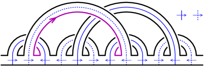
Figure 1. One possible $S_{0}$ for the word $w=aba^{-1}b^{-1}$, with outer boundary $w^{3}$. There are four turns, indicated by the numbers, each occurring three times. The boundary arc $\alpha$ leads from turn $2$ to turn $3$. This surface leads to an estimate $\operatorname{scl}(w)\leqslant 1/2$ (and in fact is extremal).

How large can $\chi(S)$ be? Note that $\chi(S)=\chi(S_{0})+\chi(S_{1})$ since $S_{0}$ and $S_{1}$ meet along circles. Also,

$$\chi(S_{0})\ =\ \frac{-n(S)\left|{w}\right|}{2}$$

as can be seen by counting the $1$–handles meeting $\partial S$: each $1$–handle contributes $-1$ to $\chi(S_{0})$ and occupies two edges in $\partial S$, of which there are $n(S)\left|{w}\right|$ in total. Finally, given $S_{0}$, the quantity $\chi(S_{1})$ is largest when $S_{1}$ is a collection of disks. The number of disks is simply the number of components of $\partial^{-}S_{0}$. We can always replace $S_{1}$ by disks, since each component of $\partial S_{1}$ maps to a vertex of $X$ and disks can be mapped to vertices also. Thus, after this modification, we have

(2) $$\chi(S)\ =\ \frac{-n(S)\left|{w}\right|}{2}\ +\ \left|{\pi_{0}(\partial^{-}S_{0})}\right|,$$

and therefore an upper bound for $\operatorname{scl}(w)$ is given by

(3) $$\frac{-\chi(S)}{2n(S)}\ =\ \frac{\left|{w}\right|}{4}\ -\ \frac{\left|{\pi_{0}(\partial^{-}S_{0})}\right|}{2n(S)}.$$

Indeed, $\operatorname{scl}(w)$ is precisely the infimum of the right hand side of (3) over all surfaces $S_{0}$ arising as above. (Note that $n(S)$ is determined by $S_{0}$.) Equation (3) essentially replaces the quantity $\chi(S)$ by the number of inner boundary components of $S_{0}$ in the computation of $\operatorname{scl}(w)$.

4. The turn graph

To help keep track of the inner boundary $\partial^{-}S_{0}$, we define the turn graph. Consider the word $w=x_{1}\cdots x_{\ell}$. A turn in $w$ is a position between two letters of $w$ considered as a cyclic word. Turns are indexed by the numbers $1$ through $\ell$, with turn $i$ being the position just after the letter $x_{i}$. Each turn is labeled by the length two subword $x_{i}x_{i+1}$ (or $x_{\ell}x_{1}$) of $w$ which straddles the turn. Note that turns are not necessarily determined by their labels.

The turn graph $\Gamma(w)$ is a directed graph with vertices equal to the turns of $w$, and with a directed edge from turn $i$ to turn $j$ if $x_{i}^{-1}=x_{j+1}$. That is, if the label of a turn begins with the letter $a^{\pm 1}$, then there is a directed edge from this turn to every other turn whose label ends with $a^{\mp 1}$. Note that because $w$ is cylically reduced, $\Gamma(w)$ has no loops.

The turn graph has a two-fold symmetry, or duality: if $e\in\Gamma(w)$ is an edge from turn $i$ to turn $j$, then one verifies easily that there is also an edge $\bar{e}$ from turn $j+1$ to turn $i-1$, and moreover $\bar{\bar{e}}=e$. Figure 2 shows a turn graph and a dual edge pair.

1pt * $ab$ at 111 188 * $ba$ at 155 176 * $ab$ at 187 144 * $b\bar{a}$ at 198 101 * $\bar{a}\bar{b}$ at 187 57 * $\bar{b}a$ at 155 25 * $a\bar{b}$ at 111 13 * $\bar{b}\bar{a}$ at 67 25 * $\bar{a}b$ at 35 57 * $b\bar{a}$ at 23 101 * $\bar{a}\bar{b}$ at 35 144 * $\bar{b}a$ at 67 176 $1$ [l] at 126 188 $2$ [l] at 170 176 $3$ [l] at 202 144 $4$ [l] at 213 101 $5$ [l] at 202 57 $6$ [l] at 170 25 $7$ [l] at 126 13 $8$ [r] at 52 25 $9$ [r] at 20 57 $10$ [r] at 8 101 $11$ [r] at 20 144 $12$ [r] at 52 176

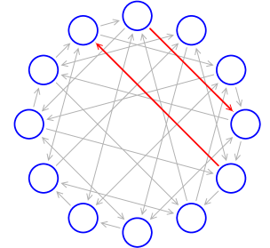
Figure 2. The turn graph for the word $w=abab\bar{a}\bar{b}a\bar{b}\bar{a}b\bar{a}\bar{b}$ (bar denotes inverse). The highlighted edges form a dual pair.

Turn circuits

Given the surface $S_{0}$, each inner boundary component can be described as follows. Traversing the curve in the positively oriented direction, one alternately follows $1$–handles and visits turns of $w$ positioned along $\partial S$; see again Figure 1 (this situation is the reason for the word “turn”). If a $1$–handle leads from turn $i$ to turn $j$, then the $1$–handle bears the transverse label $x_{i}^{-1}=x_{j+1}$, and so there is an edge in $\Gamma(w)$ from turn $i$ to turn $j$. The sequence of $1$–handles traversed by the boundary component therefore yields a directed circuit in $\Gamma(w)$. In this way the inner boundary $\partial^{-}S_{0}$ gives rise to a finite collection (possibly with repetitions) of directed circuits in $\Gamma(w)$, called the turn circuits for $S_{0}$.

Recall that $\partial S$ is labeled by $w^{n(S)}$ (possibly spread over several components), so there are $n(S)$ occurrences of each turn on $\partial S$. The turn circuits do not contain the information of which particular instances of turns are joined by $1$–handles.

Turn surgery

There is a move one can perform on $S_{0}$ which is useful. Given two occurrences of turn $i$ in $S_{0}$, cut the collar neighborhood of $\partial S$ open along arcs positioned at the two turns, between the adjacent $1$–handles; see Figure 3.

3pt $x_{i}$ [Br] at 34 101 $x_{i}$ [Br] at 34 57 $x_{i+1}$ [tl] at 138 65 $x_{i+1}$ [tl] at 138 21 $\partial^{-}S_{0}$ [Br] at 19 121 $\partial S$ [Br] at 10 93 $\partial S$ [Br] at 10 49

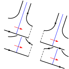
Figure 3. Cutting along two instances of turn $i$.

These arcs both map to the same vertex of $X$. Now re-glue the four sides of the arcs, switching two of them. There is one way to do this which preserves orientations of $S$ and of $\partial S_{0}$. The new surface is still admissible (that is, after capping off $\partial^{-}S_{0}$) and $n(S)$ is preserved.

The move changes both $\partial S$ and $\partial^{-}S_{0}$, in each case either increasing or decreasing the number of connected components by one. If both instances of the turn occupy the same component, then the move splits this component into two, with each occupied by one of the turns. Otherwise, the move joins the two components occupied by the turns into one.

Definition 2.

An admissible surface $S$ is taut if every component of $\partial^{-}S_{0}$ visits each turn at most once. In terms of the turn graph, this means that each turn circuit for $S_{0}$ is embedded in $\Gamma(w)$ (though distinct circuits are allowed to cross). Let ${\mathscr{T}}(w)$ be the set of taut admissible surfaces for $w$.

Any admissible surface $S$ can be made taut by performing a finite number of turn surgeries, each increasing the number of inner boundary components of $\partial S_{0}$. Since $n(S)$ remains constant, the quantity (3) will only decrease. Hence we have the following result:

Lemma 3.

There is an equality

$${\displaystyle\operatorname{scl}(w)\ \ =\ \ \inf_{S\in{\mathscr{T}}(w)}\ \frac{\left|{w}\right|}{4}\ -\ \frac{\left|{\pi_{0}(\partial^{-}S_{0})}\right|}{2n(S)}.}$$

5. Weight vectors and linear optimization

Let $\{\alpha_{1},\ldots,\alpha_{k}\}$ be the set of embedded directed circuits in $\Gamma(w)$. For each taut admissible surface $S$ let $u_{i}(S)$ be the number of occurrences of $\alpha_{i}$ among the turn circuits of $S_{0}$, and let $u(S)\in{\mathbb{R}}^{k}$ be the non-negative integer vector $(u_{1}(S),\ldots,u_{k}(S))$. We call $u(S)$ the weight vector for $S$.

For each vertex $v$ and edge $e$ of $\Gamma(w)$, there are linear functions

$$F_{v}\colon\thinspace{\mathbb{R}}^{k}\to{\mathbb{R}},\quad F_{e}\colon\thinspace{\mathbb{R}}^{k}\to{\mathbb{R}}$$

whose values on the $i^{th}$ standard basis vector $(0,\ldots,0,1,0,\ldots 0)$ are given by the number of times $\alpha_{i}$ passes through the vertex $v$ (respectively, over the edge $e$). Since $\alpha_{i}$ is embedded, these numbers will be $0$ or $1$, although this is not important. For the taut surface $S$, if $e\in\Gamma(w)$ is an edge from turn $i$ to turn $j$, then $F_{e}(u(S))$ counts the number of times $\partial^{-}S_{0}$ follows a $1$–handle from turn $i$ to turn $j$. Similarly, if $v\in\Gamma(w)$ is turn $i$, then $F_{v}(u(S))$ counts the number of occurrences of turn $i$ on $\partial^{-}S_{0}$ (which is $n(S)$, as observed earlier).

Remark 4.

For taut admissible surfaces, the functions $\left|{\pi_{0}(\partial^{-}S_{0})}\right|$ and $n(S)$ both factor as

$${\mathscr{T}}(w)\overset{u}{\longrightarrow}{\mathbb{R}}^{k}\longrightarrow{\mathbb{R}}$$

where the second map is linear, with integer coefficients. In the case of $\left|{\pi_{0}(\partial^{-}S_{0})}\right|$ the second map is given by $(u_{1},\ldots,u_{k})\mapsto\sum_{i}u_{i}$, and in the case of $n(S)$, the second map is simply $F_{v}$ (for any vertex $v\in\Gamma(w)$).

By (2) it follows that the function $-\chi(S)$ also factors as above, through an integer coefficient linear function ${\mathbb{R}}^{k}\to{\mathbb{R}}$.

Lemma 5.

Every weight vector $u(S)$ satisfies the linear equation

$$F_{e}(u(S))=F_{\bar{e}}(u(S))$$

for every dual pair $e,\bar{e}$ of edges in $\Gamma(w)$.

Proof.

Suppose $e$ leads from turn $i$ to turn $j$ (so $\bar{e}$ leads from turn $j+1$ to turn $i-1$). If a $1$–handle has a boundary arc representing $e$ then the other side of the $1$–handle represents $\bar{e}$. Hence both sides of the equation count the number of $1$–handles of $S_{0}$ joining occurrences of $x_{i}$ and $x_{j+1}$ in $\partial S$. ∎

This lemma has a converse:

Proposition 6.

If $u\in{\mathbb{R}}^{k}-\{0\}$ has non-negative integer entries and satisfies the linear equations

(4) $$F_{e}(u)=F_{\bar{e}}(u)\ \ \text{ for all dual pairs }e,\bar{e}$$

then $u$ is the weight vector of a taut admissible surface.

Proof.

Suppose $u=(u_{1},\ldots,u_{k})$. For each $i$ let $D_{i}$ be a polygonal disk with $\left|{\alpha_{i}}\right|$ sides. Label the oriented boundary of $D_{i}$ by the edges and vertices of $\alpha_{i}$. That is, sides are labeled by edges of $\Gamma(w)$, and corners are labeled by turns. Note that there are no monogons, since $\Gamma(w)$ has no loops. To form the taut admissible surface $S$, take $u_{i}$ copies of $D_{i}$ for each $i$. For each dual edge pair $e$, $\bar{e}$ the total number of edges labeled $e$ among the $D_{i}$’s will equal the number of edges labeled $\bar{e}$, by (4). Hence the sides of the disks can be joined in dual pairs to form a closed oriented surface.

However, this is not how $S$ is formed. Instead, whenever two disks were to be joined along sides labeled $e$ and $\bar{e}$, insert an oriented rectangle, with sides labeled by $e$, $x_{j+1}$, $\bar{e}$, $x_{i}$ (here, $e$ leads from turn $i$ to turn $j$, and $\bar{e}$ from turn $j+1$ to turn $i-1$). See Figure 4. The opposite sides labeled by $e$ and $\bar{e}$ are joined to the appropriate sides of the disks, and the remaining two sides become part of the boundary of $S$. Each rectangle can be transversely labeled by a fundamental groupoid generator (equal to $x_{i}^{-1}=x_{j+1}$), and then the rectangles become $1$–handles in the resulting surface $S$.

$\partial S$ [r] at 36 65 $e$ [r] at 140 71 $\bar{e}$ [l] at 193 71 $x_{j+1}$ [t] at 166 22 $x_{i}$ [b] at 166 122 * $x_{i+1}$ at 138 143 $\partial S$ [r] at 155 3 $\partial S$ [l] at 172 143 * $i$ at 136 104 * $i-1$ at 205 114 * $j+1$ at 205 32 * $j$ at 136 29 * $i+1$ at 95 157

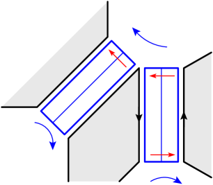
Figure 4. Building $S$ from $(u_{1},\ldots,u_{k})$.

Note that the side of a rectangle labeled $x_{i}$ has neighboring polygonal disk corners labeled $i-1$ and $i$. Following this edge along $\partial S$, the next edge must be labeled $x_{i+1}$ (adjacent to $i$ and $i+1$); see again Figure 4. Hence each component of $\partial S$ is labeled by a positive power of $w$. There are no $S^{2}$ components since no component of $S$ is closed, and no $D^{2}$ components, since an outermost $1$–handle on such a disk would have to bound a monogon. The map $S\to X$ is defined on the rectangles according to the transverse labels (each maps to an edge of $X$) and the disks map to vertices. Now $S$ is admissible, and by construction, the turn circuits will all be instances of the circuits $\alpha_{i}$, so $S$ is taut. ∎

Theorem 7 (Calegari).

If $X$ is a graph and $a\in[\pi_{1}(X),\pi_{1}(X)]$ then there exists an extremal surface $S\to X$ for $a$. Moreover, there is an algorithm to construct $S$. In particular, $\operatorname{scl}(a)$ is rational and computable.

Proof.

Let $w$ be the cyclically reduced word representing the conjugacy class of $a$, as defined in Section 3. By Remark 4 the function $\frac{-\chi(S)}{2n(S)}$ factors as

$${\mathscr{T}}(w)\overset{u}{\longrightarrow}{\mathbb{R}}^{k}{\longrightarrow}{\mathbb{R}}$$

where the second map is a ratio of linear functions $A(u)/B(u)$ with integer coefficients. Let $P\subset{\mathbb{R}}^{k}$ be the polyhedron defined by the (integer coefficient) linear equations (4) and the inequalities $B(u)>0$ and $u_{i}\geqslant 0$, $i=1,\ldots,k$. Lemma 5 and Proposition 6 together imply that the image of $u\colon\thinspace{\mathscr{T}}(w)\to{\mathbb{R}}^{k}$ is precisely $P\cap{\mathbb{Z}}^{k}$. Hence

$$\operatorname{scl}(w)\ \ =\ \ \inf_{u\in P\cap{\mathbb{Z}}^{k}}\ {A(u)}/{B(u)}.$$

Note that $P$ and $A(u)/B(u)$ are projectively invariant. Normalizing $B(u)$ to be $1$, we have

(5) $$\operatorname{scl}(w)\ \ =\ \ \inf_{u\in P^{\prime}\cap{\mathbb{Q}}^{k}}\ A(u)$$

where $P^{\prime}$ is the rational polyhedron $P\cap B^{-1}(1)$. Note that $P^{\prime}$ is a closed set.

From Remark 4 and equation (2) the function $A$ is given by

$$A(u)\ \ =\ \ \frac{\left|{w}\right|}{2}F_{v}(u)+\sum_{i}u_{i}\,,$$

which has strictly positive values on the standard basis vectors. Hence $A$ achieves a minimum on $P^{\prime}$, along a non-empty rational sub-polyhedron. The vertices of this sub-polyhedron are rational points realizing the infimum in (5). Hence there exist extremal surfaces for $w$, and $\operatorname{scl}(w)$ is rational. An extremal surface can be constructed explicitly from a rational solution $u\in P^{\prime}\cap{\mathbb{Q}}^{k}$, by first multiplying by an integer to obtain a minimizer for $A(u)/B(u)$ in $P\cap{\mathbb{Z}}^{k}$, and then applying the procedure given in the proof of Proposition 6. Lastly, we note that from the word $w$ it is straightforward to algorithmically construct the turn graph $\Gamma(w)$, the equations (4), and the polyhedron $P^{\prime}$. ∎

References

- [1] Noel Brady and Max Forester, Density of isoperimetric spectra, Geom. Topol. 14 (2010), no. 1, 435–472. MR 2578308
- [2] S. Buoncristiano, C. P. Rourke, and B. J. Sanderson, A geometric approach to homology theory, Cambridge University Press, Cambridge, 1976, London Mathematical Society Lecture Note Series, No. 18. MR 0413113 (54 #1234)
- [3] Danny Calegari, scl, MSJ Memoirs, vol. 20, Mathematical Society of Japan, Tokyo, 2009. MR 2527432
- [4] by same author, Stable commutator length is rational in free groups, J. Amer. Math. Soc. 22 (2009), no. 4, 941–961. MR 2525776
- [5] Marc Culler, Using surfaces to solve equations in free groups, Topology 20 (1981), no. 2, 133–145. MR 605653 (82c:20052)
- [6] C. P. Rourke, Presentations and the trivial group, Topology of low-dimensional manifolds (Proc. Second Sussex Conf., Chelwood Gate, 1977), Lecture Notes in Math., vol. 722, Springer, Berlin, 1979, pp. 134–143. MR 547460 (81a:57001)
- [7] John R. Stallings, A graph-theoretic lemma and group-embeddings, Combinatorial group theory and topology (Alta, Utah, 1984), Ann. of Math. Stud., vol. 111, Princeton Univ. Press, Princeton, NJ, 1987, pp. 145–155. MR 895613 (88k:20056)