Secondary structure formation of homopolymeric single-stranded nucleic acids including force and loop entropy: implications for DNA hybridization

Abstract

Loops are essential secondary structure elements in folded DNA and RNA molecules and proliferate close to the melting transition. Using a theory for nucleic acid secondary structures that accounts for the logarithmic entropy $-c\ln m$ for a loop of length $m$, we study homopolymeric single-stranded nucleic acid chains under external force and varying temperature. In the thermodynamic limit of a long strand, the chain displays a phase transition between a low temperature / low force compact (folded) structure and a high temperature / high force molten (unfolded) structure. The influence of $c$ on phase diagrams, critical exponents, melting, and force extension curves is derived analytically. For vanishing pulling force, only for the limited range of loop exponents $2<c\lesssim 2.479$ a melting transition is possible; for $c\leq 2$ the chain is always in the folded phase and for $2.479\lesssim c$ always in the unfolded phase. A force induced melting transition with singular behavior is possible for all loop exponents $c<2.479$ and can be observed experimentally by single molecule force spectroscopy. These findings have implications for the hybridization or denaturation of double stranded nucleic acids. The Poland-Scheraga model for nucleic acid duplex melting does not allow base pairing between nucleotides on the same strand in denatured regions of the double strand. If the sequence allows these intra-strand base pairs, we show that for a realistic loop exponent $c\approx 2.1$ pronounced secondary structures appear inside the single strands. This leads to a lower melting temperature of the duplex than predicted by the Poland-Scheraga model. Further, these secondary structures renormalize the effective loop exponent ${\hat{c}}$, which characterizes the weight of a denatured region of the double strand, and thus affect universal aspects of the duplex melting transition.

1 Introduction

Ribonucleic acids continue to stay in the focus of experimentalists and theorists Gesteland2005 . The advance of single molecule techniques Smith1996 ; Liphardt2002 ; Rief1999 ; Maier2000 ; Bockelmann1997 ; Mossa2009 nowadays allows to study single chains of nucleic acids under tension and varying solution conditions and thereby yields unprecedented insights into the behavior and folding properties of these essential molecules. Theory on RNA folding vastly relies on the idea of hierarchical folding proposed by Tinoco et al. Tinoco1971 ; Tinoco1999 , stating that given a sequence (the primary structure), the secondary structure (i. e. the list of all base pairs) forms independently of the tertiary structure (the overall three-dimensional arrangement of all atoms). This is in contrast to the protein folding problem, which does not feature these well separated energy scales between the different structural levels and hence is more involved Finkelstein2004 . The idea of hierarchical folding therefore suggests to solely focus on the secondary structure, i. e. the base pairs, and to neglect the tertiary structure. This constitutes a major simplification and enables to calculate partition functions exactly and to predict the secondary structure formed by a given RNA sequence. De Gennes Gennes1968 was the first to calculate the partition function of an ideal homopolymeric RNA chain by using a propagator formalism and solving the partition function by means of a singularity analysis of the generating functions. Due to his real space approach for an ideal polymer, the loop exponent was fixed at $c=3/2$. The loop exponent $c$ characterizes the logarithmic entropy contribution $\propto\ln m^{-c}$ of a loop of length $m$. Ten years later, Waterman and Smith Waterman1978a devised a recursion relation appropriate for the partition function of folded RNA, which now lies at the heart of most RNA secondary structure and free energy prediction algorithms currently used. Since all results obtained for RNA are also valid for DNA on our relative primitive level of modeling, we will mostly explicitly refer to RNA in our paper but note that in principle all our results carry over to single stranded DNA molecules, as well. Subsequently, several theoretical models were developed to study RNA and DNA: those were focused on melting Einert2008 ; Hofacker1994 ; McCaskill1990 , stretching Einert2010 ; Montanari2001 ; Gerland2001 ; Mueller2002 ; Hanke2008 ; Cocco2002a , unzipping Lubensky2002 , translocation Bundschuh2005 , salt influence Einert2010a ; Tan2006 ; Mamasakhlisov2007 , pseudoknots Baiesi2003 ; Orland2002 , and the influence of the loop exponent Einert2008 ; Einert2010 ; Blossey2003 ; Kafri2000 . In this context, an interesting question in connection with the melting of double stranded DNA (dsDNA) arises: Do secondary structure elements form in the single strands inside denatured dsDNA loops or not? Formation of such secondary structures in dsDNA loops would mean that inter-strand base pairing between the two strands – being responsible for the assembly of the double helix – is in competition with intra-strand pairing, where bases of the same strand interact. This question is not only important for the thermal melting of dsDNA but also for DNA transcription, DNA replication and the force-induced overstretching transition of DNA Alberts2002 ; Rief1999 .

In this paper, the influence of the loop exponent $c$ on the behavior of RNA subject to varying temperature and external force is studied, which goes beyond our previous work where only the temperature influence was considered Einert2008 . We neglect sequence effects and consider a long homopolymeric, single stranded RNA molecule. A closed form expression for the partition function is derived, which allows to study the thermodynamic behavior in detail. The phase diagram in the force-temperature plane is obtained. We find that the existence of a temperature induced phase transition depends crucially on the value of the loop exponent $c$: at vanishing force a melting transition is possible only for the limited range of loop exponents $2<c<2.479$. $c\approx 2.1$ is a typical exponent that characterizes the entropy of loops usually encountered in RNA structures – hairpin loops, internal loops, multi-loops with three or more emerging helices. That means that RNA molecules are expected to experience a transition between a folded and an unfolded state. This is relevant for structure formation in DNA or RNA single strands and can in principle be tested in double laser trap force clamp experiments Gebhardt2010 . Our findings also have implications for the denaturation of double helical nucleotides (e. g. dsDNA). Since intra-strand and inter-strand base pairing compete, secondary structure formation of the single strands inside denatured regions of the duplex has to be taken into account in a complete theory of dsDNA melting. In the case where intra- and inter-strand base pairing occurs, the classical Poland-Scheraga mechanism for the melting of a DNA duplex has to be augmented by the single-strand folding scenario considered by us, as the Poland-Scheraga theory is only valid in the case where no intra-strand base pairing is possible. If the intra-strand interactions are strong enough to induce folded secondary structures, we show that the loop exponent governing the entropy of inter-strand loops is renormalized and takes on an effective universal value that only depends on whether the inter-strand loops are symmetric (consisting of two strands of the same length) or asymmetric. The resulting duplex melting transition is universal and turns out to be strongly discontinuous in the first, symmetric case, and on the border between continuous and discontinuous in the second, asymmetric case. In the case when intra-strand base pairing is weak and a single strand is in the unfolded phase, the situation is different and qualitatively similar to the original Poland-Scheraga results, yet with a lower melting temperature. All these effects can be studied experimentally. We make explicit suggestions for dsDNA sequences, with which the formation of intra-strand secondary structures inside inter-strand loops can be selectively inhibited or favored.

2 Derivation of partition function

2.1 Model

Single stranded RNA is modeled as a one-dimensional chain. The basic units are nucleotides with the four bases (cytosine (C), adenine (A), guanine (G), uracil (U)), which are enumerated by an index $i=1,\ldots,N$. A nucleotide can establish a base pair (bp) with another nucleotide via hydrogen bonding, leading to helices and loops as the structural building blocks of an RNA secondary structure, see fig. 1. In agreement with previous treatments, a valid secondary structure is a list of all base pairs with the constraint that a base can be part of at most one pair. In addition, pseudoknots are not allowed, that means that for any two base pairs $(i,j)$ and $(k,l)$ with $i<j$, $k<l$, and $i<k$ we have either $i<k<l<j$ or $i<j<k<l$ Orland2002 . This imposes a hierarchical order on the base pairs, meaning that two base pairs are either nested and part of the same substructure or are independent and part of different substructures, fig. 2. Helix stacking – the interaction of two helices emerging from the same loop – and base triples as well as the overall three-dimensional structure are not considered. Base pairs are stabilized by two different interactions. First, by hydrogen bonds between complementary bases and, second, by the stacking interaction between neighboring base pairs, which are accounted for by the sequence independent parameters $g_{\mathrm{h}}^{\mathrm{hb}}$ and $g_{\mathrm{h}}^{\mathrm{stack}}$, respectively. A helix with $h$ base pairs consequently has the free energy $h(g_{\mathrm{h}}^{\mathrm{hb}}+g_{\mathrm{h}}^{\mathrm{stack}})-g_{\mathrm{h}}^{\mathrm{stack}}+g_{\mathrm{h}}^{\mathrm{i}}$, where $g_{\mathrm{h}}^{\mathrm{i}}$ is a helix initiation free energy. Therefore, the hydrogen bonding and the stacking interaction can be combined to yield the binding energy per base pair $\varepsilon=-(g_{\mathrm{h}}^{\mathrm{hb}}+g_{\mathrm{h}}^{\mathrm{stack}})$, which we define to be positive. $\varepsilon$ can be measured experimentally by duplex hybridization Xia1998 and contains the binding free energies as well as the extensive part of configurational polymer entropy. Further, the stacking interaction appears as an additional contribution to the helix initiation free energy. We define $\mathcal{G}_{\mathrm{h}}^{\mathrm{init}}=g_{\mathrm{h}}^{\mathrm{i}}-g_{\mathrm{h}}^{\mathrm{stack}}$ and describe the binding free energy by a single, sequence independent parameter Einert2008

$$w=\exp(\varepsilon/(\mathrm{k_{B}}T))\;.$$ (1)

$w$ is the statistical weight of a bound base pair, $T$ is the absolute temperature, and $\mathrm{k_{B}}$ the Boltzmann constant. Therefore this is a model for homopolymeric RNA, which can be realized experimentally with synthetic alternating sequences $[\mathrm{AU}]_{N/2}$ or $[\mathrm{GC}]_{N/2}$. It has also been argued that this homopolymeric model describes random RNA above the glass transition Bundschuh2002a .

The non-extensive contribution of the free energy of a loop is given by

$$\mathcal{G}_{\mathrm{l}}^{\mathrm{conf}}=-\mathrm{k_{B}}T\ln m^{-c}$$ (2)

and describes the entropy difference between an unconstrained polymer and a looped polymer. The loop exponent $c$ is $c_{\mathrm{ideal}}=3/2$ for an ideal polymer and $c_{\mathrm{SAW}}=d\nu\simeq 1.76$ for an isolated self avoiding loop with $\nu\simeq 0.588$ in $d=3$ dimensions Gennes1979 . However, helices, which emerge from the loop, increase $c$ even further. In the asymptotic limit of long helical sections, renormalization group predicts $c_{l}=d\nu+\sigma_{l}-l\sigma_{3}$ for a loop with $l$ emerging helices Duplantier1986 ; Kafri2000 , where $\sigma_{l}=\epsilon l(2-l)/16+\epsilon^{2}l(l-2)(8l-21)/512+\mathcal{O}(\epsilon^{3})$ in an $\epsilon=4-d$ expansion. One obtains $c_{1}=2.06$ for terminal, $c_{2}=2.14$ for internal loops and $c_{4}=2.16$ for a loop with four emerging helices. For larger $l$ the $\epsilon$ expansion prediction for $c_{l}$ becomes unreliable. One sees that the variation of $c$ over different loop topologies that appear in the native structures of RNA is quite small, which justifies our usage of the same exponent $c$ for loops of all topologies that occur in a given RNA secondary structure.

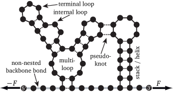
Figure 1: Schematic representation of the secondary structure of an RNA molecule. Dots represent one base, i. e. cytosine, guanine, adenine, or uracil. Solid lines denote the sugar-phosphate backbone bonds, broken lines base pairs, and thick gray lines the non-nested backbone bonds, which are counted by the variable $M$, here $M=11$. The thick arrows to either side illustrate the force $F$ applied to the 5’- and 3’-end.

Figure 2: The arc diagram is a representation of the secondary structure depicted in fig. 1. A dot represents one base. Solid lines denote the backbone bonds and thick gray lines the non-nested backbone bonds. Dashed arcs denote hydrogen bonds between two bases. A pseudoknot (dotted arc) is recognized here as crossing arcs. If no pseudoknots are present the structure is hierarchical, meaning that substructures are either nested or juxtaposed.

2.2 Canonical partition function

Figure 3: Illustration of the recursion scheme for the canonical partition function in eq. (3). Boxes denote partition functions of substrands (the range is given by the subindices). The numbers inside a box give the number of non-nested backbone bonds. To calculate the partition function of a strand ranging from $i$ through $j+1$, consider the partition function of a strand ranging from $i$ through $j$ and add base number $j+1$, which may (right term in first row) or may not (left term in first row) establish a base pair with base number $k$. In the second row $Q_{k,j+1}^{0}$ is calculated by closing structures with $m$ non-nested bonds with a hydrogen bond (dashed line). For homopolymeric RNA, the sequence dependence drops out and only the lengths of the substrands, $N=j-i$, $n=k-1-i$, $N-n=j+1-k$, need to be considered, see eq. (3).

As we neglect pseudoknots, only hierarchical structures are present, which allows to write down a recursion relation for the partition function. Further, as we consider homopolymers and omit sequence effects by using a constant base pairing weight $w$, the system is translationally invariant. Hence, the canonical partition function $Q_{i,j}^{M}$ of a strand ranging from base $i$ at the 5’-end through $j$ at the 3’-end depends only on the total number of segments $N=j-i$ and on the number of non-nested backbone bonds $M$. A non-nested bond is defined as a backbone bond, which is neither part of a helix nor part of a loop. It is outside all secondary structure elements and therefore contributes to the end-to-end extension, which couples to an external stretching force and which can be observed for example in force spectroscopy experiments Einert2008 ; Bundschuh2005 ; Mueller2003 , see figs. 1 and 2. The recursion relations for $Q_{N}^{M}$ can be written as

$$Q_{N+1}^{M+1}=\frac{v_{\mathrm{f}}(M+1)}{v_{\mathrm{f}}(M)}\left[Q_{N}^{M}+w\sum_{n=M}^{N-1}Q_{n}^{M}Q_{N-n}^{0}\right]$$ (3a)

and

$$Q_{N-n}^{0}=\sum_{m=-1}^{N-n-2}\frac{Q_{N-n-2}^{m}}{v_{\mathrm{f}}(m)}\frac{\exp\bigl{(}-\mathcal{G}_{\mathrm{h}}^{\mathrm{init}}\Theta({m-2})/(\mathrm{k_{B}}T)\bigr{)}}{(m+2)^{c}}\;$$ (3b)

and is illustrated in fig. 3. The Heaviside step function is $\Theta({m})=0$ if $m\leq 0$ and $\Theta({m})=1$ if $m>0$. Eq. (3a) describes the elongation of an RNA structure by either adding an unpaired base (first term) or by adding an arbitrary substrand $Q_{N-n}^{0}$ that is terminated by a helix. Eq. (3b) constructs $Q_{N-n}^{0}$ by closing structures with $m$ non-nested bonds, summed up in $Q_{N-n-2}^{m}$, by a base pair. $v_{\mathrm{f}}(M)$ denotes the number of configurations of a free chain with $M$ links and can be completely eliminated from the recursion relation by introducing the rescaled partition function $\tilde{Q}_{N}^{M}=Q_{N}^{M}/v_{\mathrm{f}}(M)$. We set $\mathcal{G}_{\mathrm{h}}^{\mathrm{init}}=0$ for computational simplicity and combine eqs. (3a) and (3b), which leads to the final recursion relation

$$\tilde{Q}_{N+1}^{M+1}=\tilde{Q}_{N}^{M}+w\sum_{n=M}^{N-1}\sum_{m=-1}^{N-n-2}\frac{\tilde{Q}_{n}^{M}\tilde{Q}_{N-n-2}^{m}}{(m+2)^{c}}\;,$$ (4)

with the boundary conditions $\tilde{Q}_{-1}^{-1}=1$, $\tilde{Q}_{M}^{N}=0$ for $M>N$, $N<0$, or $M<0$. The thermodynamic limit of an infinitely long RNA chain is described by the canonical Gibbs ensemble, which is characterized by a fixed number of segments $N$, but a fluctuating number of non-nested backbone bonds $M$. Therefore we introduce the unrestricted partition function

$$Z_{N}(s)=\sum_{M=0}^{\infty}s^{M}\tilde{Q}_{N}^{M}\;,$$ (5)

which contains the influence of an external force $F$ via the statistical weight $s$ of a non-nested backbone bond. For RNA with no force applied to the ends, one has $s=1$. We model the RNA backbone elasticity by the freely jointed chain (FJC) model, where the weight of a non-nested backbone bond subject to an external force is given by

$$s=\frac{1}{4\pi}\int_{0}^{2\pi}\mathrm{d}\phi\int_{0}^{\pi}\mathrm{d}\theta\,\mathrm{e}^{-\beta Fb_{\mathrm{ss}}\cos\theta}=\frac{\sinh(\beta Fb_{\mathrm{ss}})}{\beta Fb_{\mathrm{ss}}}\;;$$ (6)

here, we introduced the inverse thermal energy $\beta=(\mathrm{k_{B}}T)^{-1}$ and the Kuhn length $b_{\mathrm{ss}}$.

2.3 Grand canonical partition function

For studying the phase transition and the critical behavior, it is useful to introduce the generating function or grand canonical partition function

$$\mathcal{Z}(z,s)=\sum_{N=0}^{\infty}z^{N}Z_{N}(s)=\sum_{N=0}^{\infty}\sum_{M=0}^{\infty}z^{N}s^{M}\tilde{Q}_{N}^{M}\;,$$ (7)

where $z=\exp(\mu/(\mathrm{k_{B}}T))$ is the fugacity.

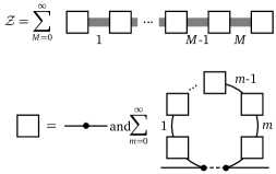
Figure 4: Structure of the grand canonical partition function $\mathcal{Z}(z,s)$ according to eqs. (7) and (11). The grand canonical partition function of the Gibbs ensemble is a sum over all numbers of non-nested backbone bonds (thick gray lines) with statistical weight $sz$. Between two adjacent backbone bonds can be either a single nucleotide (dot), with statistical weight $1$, or a structure with weight $\mathcal{Z}_{\mathrm{b}}$, whose first and last base are paired. The white squares serve as wildcards for either possibility and have the statistical weight $\kappa(w,z)$. Thin black lines depict backbone bonds that are part of a helix or loop and have statistical weight $z$.

Performing the weighted double sum $\sum_{N=-1}^{\infty}\sum_{M=-1}^{\infty}z^{N}s^{M}$ on both sides of eq. (4) yields

$$(sz)^{-1}\mathcal{Z}=(sz)^{-1}+\mathcal{Z}+\bigl{(}(sz)^{-1}+\mathcal{Z}\bigr{)}(\kappa-1)\;,$$ (8)

which can be solved and one obtains the generating function

$$\mathcal{Z}(z,s)=\frac{\kappa(w,z)}{1-sz\kappa(w,z)}\;.$$ (9)

Here we have defined $\kappa(w,z)=1+\mathcal{Z}_{\mathrm{b}}(w,z)$ as the grand canonical partition function of RNA structures with zero non-nested backbone bonds, i. e. structures which consist of just one nucleotide or structures where the terminal bases are paired,

$$\kappa(w,z)=1+\mathcal{Z}_{\mathrm{b}}(w,z)=1+wz^{2}\sum_{N=-1}^{\infty}\sum_{M=-1}^{N}z^{N}\frac{\tilde{Q}_{N}^{M}}{(M+2)^{-c}}\;.$$ (10)

Eq. (9) has an instructive interpretation, which becomes clear by expanding the fraction in a geometric series

$$\mathcal{Z}(z,s)=\sum_{M=0}^{\infty}s^{M}\,z^{M}\kappa^{M+1}=\sum_{M=0}^{\infty}(1+\mathcal{Z}_{\mathrm{b}})\cdot\bigl{(}sz(1+\mathcal{Z}_{\mathrm{b}})\bigr{)}^{M}\;,$$ (11)

where $sz$ is the statistical weight for a backbone segment which is not nested. Between two adjacent segments we have the possibility to put either a single nucleotide (with statistical weight $1$) or a structure whose first and last bases are paired (with statistical weight $\mathcal{Z}_{\mathrm{b}}$). See fig. 4 for an illustration.

In order to determine the function $\kappa(w,z)$, we compare the coefficients of the power series in $s$ in eqs. (7) and (11) and obtain $z^{M}\kappa^{M+1}=\sum_{N=M}^{\infty}z^{N}\tilde{Q}_{N}^{M}$. The lower summation index is due to exchanging the summations in eq. (7), bearing in mind that $\tilde{Q}_{N}^{M}=0$ for $M>N$. This identity can be inserted into eq. (10) and yields the equation

$$\kappa(w,z)-1=\frac{w}{\kappa(w,z)}\mathrm{Li}_{c}(z\kappa(w,z))\;,$$ (12)

which determines $\kappa(w,z)$. $\mathrm{Li}_{c}(z\kappa)=\sum_{m=1}^{\infty}z^{m}\kappa^{m}/m^{c}$, for $z\kappa\leq 1$, is the polylogarithm Erdelyi1953 . We introduce

$$h(\kappa,z)=\frac{w}{\kappa}\mathrm{Li}_{c}(z\kappa)\;$$ (13)

and rewrite eq. (12) as $\kappa-1=h(\kappa,z)$. Eq. (12) has at most two positive and real solutions as can be seen from fig. 5, where we plot the two sides of eq. (12). $\kappa(w,z)$ is a continuous, monotonically increasing function of $z$ with $\kappa(w,0)=1$ as follows from eq. (10). Therefore, only the smallest positive root of eq. (12) yields the correct $\kappa(w,z)$. For $z\rightarrow 0$ there is always a positive and real solution for $\kappa(w,z)$. Increasing $z$ increases $\kappa(w,z)$ until eventually, at $z=z_{\mathrm{b}}$, the real solution for $\kappa(w,z)$ vanishes. Thus, $\kappa(w,z)$ has a branch point at $z=z_{\mathrm{b}}$. Depending on the value of the loop exponent $c$, the polylogarithm $\mathrm{Li}_{c}(z\kappa)$ and $h(\kappa,z)$ (a) are divergent for $c\leq 1$, (b) are finite, but feature a diverging slope for $1<c\leq 2$, or (c) have a finite value and derivative for $2<c$ at $z\kappa=1$, see fig. 5. This will become important later, when the existence of phase transitions is studied.

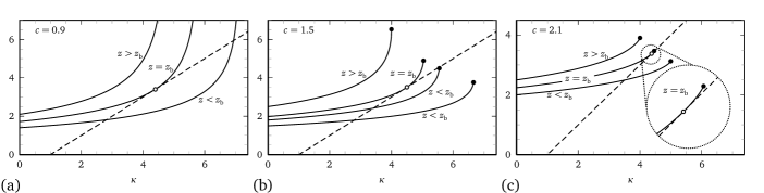
Figure 5: Graphical solution of the equations, which determine $\kappa(w,z)$, $z_{\mathrm{b}}$, $z_{\mathrm{p}}$. The functions $\kappa-1$ (dashed line) and $h(\kappa,z)$ (solid lines), eq. (13), are plotted for $w=10$ and different values of the fugacity $z$ and the loop exponent $c$, (a) $c=0.9$ (b) $c=3/2$ (c) $c=2.1$. Points at which both curves intersect are solutions of eq. (12) and determine $\kappa(w,z)$. In case of two positive solutions the smaller yields the correct solution as $\kappa(w,z)$ is to be a continuous, monotonically increasing function of $z$ with $\kappa(w,0)=1$, eq. (10). Points at which both curves are adjacent to each other (open circles) determine the branch point $z_{\mathrm{b}}$. Points at which $z\kappa=1$ (filled circles) determine the position of the pole $z_{\mathrm{p}}$ in the absence of force, $s=1$.

2.4 Back-transform to canonical ensemble

Since the thermodynamic limit $N\rightarrow\infty$ is defined in the canonical Gibbs ensemble, we now demonstrate how to obtain $Z_{N}(s)$, eq. (5), from $\mathcal{Z}(z,s)$, eq. (9). For large systems, $N\gg 1$, the canonical partition function is given by the dominant singularity $z_{\mathrm{d}}(s)$ of $\mathcal{Z}(z,s)$, which is defined as the singularity which is nearest to the origin in the complex $z$-plane Flajolet1990 ; Einert2010 . In particular if $\mathcal{Z}(z,s)\sim K(s)\bigl{(}z_{\mathrm{d}}(s)-z\bigr{)}^{-\alpha}$ with $K(s)$ independent of $z$, we obtain

$$Z_{N}(s)\sim z_{\mathrm{d}}^{-N}(s)N^{\alpha-1}\cdot K(s)z_{\mathrm{d}}^{-\alpha}(s)/\Gamma(\alpha)\;,$$ (14)

where $\Gamma(\alpha)$ is the gamma function Abramowitz2002 . Therefore, the Gibbs free energy reads to leading orders in $N$

$$\mathcal{G}/(\mathrm{k_{B}}T)=-\ln Z_{N}\sim N\ln z_{\mathrm{d}}(s)+(1-\alpha)\ln N\;.$$ (15)

In fact, $\mathcal{Z}(z,s)$ features two relevant singularities. First, the branch point $z_{\mathrm{b}}(w)$ of $\kappa(w,z)$, which is independent of $s$, and second a simple pole $z_{\mathrm{p}}(w,s)$, where the denominator of $\mathcal{Z}(z,s)$ vanishes, see eq. (9). Depending on which singularity has the smallest modulus, the molecule can be in different phases. In the following sections it will turn out that the low temperature, compact or folded phase is associated with $z_{\mathrm{b}}$, whereas the high temperature, extended or unfolded phase is characterized by $z_{\mathrm{p}}$.

Let us consider the branch point first. It can be seen from fig. 5, that for $z<z_{\mathrm{b}}$ at least one real solution of eq. (12) exists, where the smaller solution determines $\kappa(w,z)$. Right at $z=z_{\mathrm{b}}$ the two solutions merge and the slope of $h$ is $h^{\prime}(\kappa,z_{\mathrm{b}})=\partial h(\kappa,z_{\mathrm{b}})/\partial\kappa=1$ at the tangent point. This yields the equation for the position of the branch point singularity $z_{\mathrm{b}}(w)$, which is a function of $w$ only,

$$\kappa(w,z_{\mathrm{b}})^{2}=w\mathrm{Li}_{c-1}(z_{\mathrm{b}}\kappa(w,z_{\mathrm{b}}))-w\mathrm{Li}_{c}(z_{\mathrm{b}}\kappa(w,z_{\mathrm{b}}))\;.$$ (16)

The behavior of $\kappa(w,z)$ in the vicinity of the branch point can be obtained by expanding eq. (12) for $z\rightarrow z_{\mathrm{b}}$ and $z_{\mathrm{b}}\kappa(w,z_{\mathrm{b}})<1$

$$\kappa(w,z)\sim\kappa_{\mathrm{b}}-\Bigl{(}{\frac{z_{\mathrm{b}}-z}{z_{\mathrm{b}}}}\Bigr{)}^{1/2}K_{\mathrm{b}}{(1-sz_{\mathrm{b}}\kappa_{\mathrm{b}})^{2}}\;,$$ (17)

where we used the short notation $\kappa_{\mathrm{b}}=\kappa(w,z_{\mathrm{b}})$ and defined

$$K_{\mathrm{b}}=\Bigl{(}{\frac{2w\mathrm{Li}_{c-1}(z_{\mathrm{b}}\kappa_{\mathrm{b}})}{w\mathrm{Li}_{c-2}(z_{\mathrm{b}}\kappa_{\mathrm{b}})-w\mathrm{Li}_{c-1}(z_{\mathrm{b}}\kappa_{\mathrm{b}})-2\kappa_{\mathrm{b}}^{2}}}\Bigr{)}^{1/2}\frac{\kappa_{\mathrm{b}}}{(1-sz_{\mathrm{b}}\kappa_{\mathrm{b}})^{2}}$$ (18)

Due to the exponent $1/2$ in the above equation, the function $\kappa(w,z)$ exhibits a first order branch point at $z=z_{\mathrm{b}}$ and the grand canonical partition function, eq. (9), scales as

$$\mathcal{Z}(z,s)\sim\frac{\kappa_{\mathrm{b}}}{1-sz_{\mathrm{b}}\kappa_{\mathrm{b}}}-\Bigl{(}{\frac{z_{\mathrm{b}}-z}{z_{\mathrm{b}}}}\Bigr{)}^{1/2}K_{\mathrm{b}}\;.$$ (19)

Together with eq. (14), we obtain the following scaling for the canonical partition function

$$Z_{N}(s)\sim z_{\mathrm{b}}^{-N}N^{-3/2}K_{\mathrm{b}}/\sqrt{4\pi}\;,$$ (20)

which leads to a logarithmic $N$-contribution with universal prefactor $3/2$ to the free energy $\mathcal{G}=-\mathrm{k_{B}}T\ln Z_{N}$, in accord with the findings of de Gennes Gennes1968 . It will turn out that eq. (20) describes the low temperature or folded phase of the system.

Now let us consider the pole singularity $z_{\mathrm{p}}$ of the grand canonical partition function. $z_{\mathrm{p}}(w,s)$ is a function of $w$ and $s$ and is given by the zero of the denominator of $\mathcal{Z}(z,s)$ in eq. (9),

$$sz_{\mathrm{p}}\kappa(w,z_{\mathrm{p}})=1\;.$$ (21)

The position of the pole can be evaluated in a closed form expression by plugging eq. (21) into eq. (12) and solving the resulting quadratic equation for $z$. One obtains

$$z_{\mathrm{p}}(w,s)=\frac{2}{s}\left(1+\sqrt{1+4w\mathrm{Li}_{c}(1/s)}\right)^{-1}\;,$$ (22a)

$$\kappa(w,z_{\mathrm{p}})=\frac{1}{2}\left(1+\sqrt{1+4w\mathrm{Li}_{c}(1/s)}\right)\;.$$ (22b)

The behavior of $\kappa(w,z)$ in the vicinity of the pole can be obtained by expanding eq. (12) for $z\rightarrow z_{\mathrm{p}}$, $z_{\mathrm{p}}\kappa(w,z_{\mathrm{p}})=1/s<1$, and $c>2$

$$\kappa(w,z)\sim\kappa_{\mathrm{p}}-\kappa_{\mathrm{p}}\frac{z_{\mathrm{p}}-z}{z_{\mathrm{p}}}\ \frac{w\mathrm{Li}_{c-1}(1/s)}{K_{\mathrm{p}}(2\kappa_{\mathrm{p}}-1)}\;,$$ (23)

where we used the short notation $\kappa_{\mathrm{p}}=\kappa(w,z_{\mathrm{p}})$ and introduced

$$K_{\mathrm{p}}=\frac{2\kappa_{\mathrm{p}}^{2}-\kappa_{\mathrm{p}}-w\mathrm{Li}_{c-1}(1/s)}{2\kappa_{\mathrm{p}}-1}\;.$$ (24)

Therefore, the grand canonical partition function scales as

$$\mathcal{Z}(z,s)\sim\Bigl{(}\frac{z_{\mathrm{p}}-z}{z_{\mathrm{p}}}\Bigr{)}^{-1}K_{\mathrm{p}}\;$$ (25)

and together with eq. (14) we obtain the scaling of the canonical partition function

$$Z_{N}(s)\sim z_{\mathrm{p}}^{-N}K_{\mathrm{p}}\;.$$ (26)

Later we will see, that eq. (26) describes the denatured high temperature phase of the system. In contrast to the branch point phase, eq. (20), no logarithmic contribution to the free energy is present.

3 Critical behavior

The two singularities $z_{\mathrm{b}}(w)$ and $z_{\mathrm{p}}(w,s)$ are smooth functions of external variables such as temperature $T$ or force $F$, which enter via the weight of a base pair $w$, eq. (1), and the weight of a non-nested backbone bond $s$, eq. (6). As the system is described by the singularity, which is closest to the origin, a phase transition associated with a true singularity in the free energy, eq. (15), is possible if these two singularities cross. For that purpose let us shortly review the three constitutive equations eqs. (12),(16), and (21). As observed earlier, the smallest positive root of eq. (12) yields the function $\kappa(w,z)$. The simultaneous solution of eqs. (12) and (16) yields the branch point $z_{\mathrm{b}}(w)$, whereas the simultaneous solution of eqs. (12) and (21) yields the pole $z_{\mathrm{p}}(w,s)$, which can be expressed in a closed form, see eq. (22).

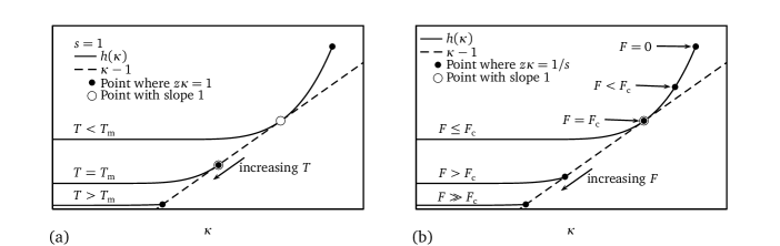
Figure 6: Illustration of the graphical solution of eqs. (12),(16), and (21) at the phase transition. The solid line sketches $h(\kappa)$, eq. (13), the dashed line the function $\kappa-1$. The open circles denote points where the conditions for the branch point are met: Curves have common points, eq. (12), and curves are tangent to each other in these points, eq. (16). The black filled circles denote points where $sz\kappa=1$, eq. (21). If the black filled circle lies on the dashed curve the conditions for a pole are met, eqs. (12) and (21). For a given temperature $T$ and force $F$ the fugacity $z$ is increased from $z=0$ to the value where either eqs. (12) and (16) hold (open circle on dashed line, folded phase) or eqs. (12) and (21) hold (black filled circle on dashed line, unfolded phase). (a) Illustration of the thermal phase transition at zero force, $s=1$. For low temperatures the branch point is dominant. Upon increasing the temperature, i. e. decreasing $w$, the branch point and the pole approach each other until they eventually coincide at the melting temperature $T=T_{\mathrm{m}}$ and cause a phase transition. For $T>T_{\mathrm{m}}$ there is no branch point anymore and the pole is dominant. (b) Illustration of the force induced phase transition at a temperature $T<T_{\mathrm{m}}$. For small forces the branch point is dominant. Upon increasing the force, i. e. increasing $s$, the point where $z\kappa=1/s$ (black filled circle) moves towards the branch point. As the branch point is independent of the force, see eqs. (12) and (16), no observable depends on $F$ as long as $F<F_{\mathrm{c}}$. At $F=F_{\mathrm{c}}$ the branch point and the pole coincide and a phase transition occurs. For $F>F_{\mathrm{c}}$ the pole is dominant.

3.1 Critical point and existence of a phase transition

The critical fugacity $z_{\mathrm{c}}$ and thus the phase transition is defined as the point where the branch point and the pole coincide

$$z_{\mathrm{c}}=z_{\mathrm{b}}(w_{\mathrm{c}})=z_{\mathrm{p}}(w_{\mathrm{c}},s_{\mathrm{c}})\;,$$ (27)

which means that all three eqs. (12),(16), and (21) have to hold simultaneously, see fig. 6. Assuming that a pair $(w_{\mathrm{c}},s_{\mathrm{c}})$ exists so that eq. (27) is true, this can be evaluated further by plugging eqs. (22) into eq. (16) and we obtain

$$w_{\mathrm{c}}=\frac{\mathrm{Li}_{c-1}(1/s_{\mathrm{c}})-\mathrm{Li}_{c}(1/s_{\mathrm{c}})}{(\mathrm{Li}_{c-1}(1/s_{\mathrm{c}})-2\mathrm{Li}_{c}(1/s_{\mathrm{c}}))^{2}}\;.$$ (28)

This constitutes a closed form relation between $w_{\mathrm{c}}$ and $s_{\mathrm{c}}$ or, by employing eqs. (1) and (6), the critical temperature $T_{\mathrm{c}}$ and force $F_{\mathrm{c}}$. The melting temperature $T_{\mathrm{m}}$ is defined as the critical temperature at zero force.

The order of the branch point exactly at $T=T_{\mathrm{m}}$ and zero force, $s=1$, is calculated by expanding eq. (12) in powers of $z/z_{\mathrm{c}}-1$ and $\kappa(w,z)/\kappa_{\mathrm{c}}-1$ while keeping $w=w_{\mathrm{c}}$ fixed. For vanishing force $\kappa_{\mathrm{c}}=1/z_{\mathrm{c}}$ and we obtain

$$\kappa(w,z)\sim\kappa_{\mathrm{c}}-\frac{\kappa_{\mathrm{c}}}{K_{\mathrm{c,T}}}\Bigl{(}\frac{z_{\mathrm{c}}-z}{z_{\mathrm{c}}}\Bigr{)}^{{1}/{(c-1)}}\;,$$ (29)

where we used

$$K_{\mathrm{c,T}}=\Bigl{(}\frac{\zeta_{c-1}}{\Gamma(1-c)}\Bigr{)}^{-1/(c-1)}\;.$$ (30)

Thus, the asymptotic behavior of the generating function at $T=T_{\mathrm{m}}$ and zero force is

$$\mathcal{Z}(z,s)\sim K_{\mathrm{c,T}}\Bigl{(}\frac{z_{\mathrm{c}}-z}{z_{\mathrm{c}}}\Bigr{)}^{-1/(c-1)}\;,$$ (31)

and we obtain the modified scaling of the canonical partition function right at the melting point temperature

$$Z_{N}({s=1})\sim z_{\mathrm{c}}^{-N}N^{(2-c)/(c-1)}{K_{\mathrm{c,T}}}/{\Gamma({1/(c-1)})}\;.$$ (32)

We see that the loop statistics are crucial and enter via the loop exponent $c$, which gives rise to non-universal critical behavior.

For finite force, $s>1$, the branch point is first order and the scaling of the generating function at the critical point reads

$$\mathcal{Z}(z,s)\sim\Bigl{(}\frac{z_{\mathrm{c}}-z}{z_{\mathrm{c}}}\Bigr{)}^{-1/2}\frac{K_{\mathrm{c,F}}}{s}\;,$$ (33)

with

$$K_{\mathrm{c,F}}=\Bigl{(}{\frac{w_{\mathrm{c}}\mathrm{Li}_{c-2}(1/s)-w_{\mathrm{c}}\mathrm{Li}_{c-1}(1/s)-2\kappa_{\mathrm{c}}^{2}}{2w_{\mathrm{c}}\mathrm{Li}_{c-1}(1/s)}}\Bigr{)}^{1/2}\;,$$ (34)

leading to the canonical partition function

$$Z_{N}({s})\sim z_{\mathrm{c}}^{-N}N^{-1/2}K_{\mathrm{c,F}}/(s\sqrt{\pi})\;,$$ (35)

with a scaling independent of the loop exponent $c$. Note that eq. (33) scales as $(z_{\mathrm{c}}-z)^{-1/2}$ in contrast to eq. (19), which leads to the different scaling of $Z_{N}({s})$ in eq. (35) when compared to eq. (20). In the rest of this section we compare thermal and force induced phase transition and in particular determine the parameter range in which a phase transition is possible.

3.1.1 Thermal phase transition

First, we consider the thermal phase transition without external force, i. e. for $s=1$. In this case the polylogarithm reduces to the Riemann zeta function, $\mathrm{Li}_{c}(1)=\zeta_{c}$. Since $s=1$, we find that $z_{\mathrm{b}}\leq z_{\mathrm{p}}$ as long as $\kappa(w,z)$ has a real, positive branch point. This is due to the fact that $z_{\mathrm{b}}\kappa(w,z_{\mathrm{b}})\leq 1$ (see fig. 5), $z_{\mathrm{p}}\kappa(w,z_{\mathrm{p}})=1$, and that $z\kappa(w,z)$ is a monotonically increasing function of $z$, see eq. (10).

No thermal phase transition for $c\leq 2$

For $c\leq 2$ the function $\kappa(w,z)$ always features a branch point since $h^{\prime}(\kappa)\rightarrow\infty$ for $\kappa\rightarrow 1/z$. This ensures that for every $w$ a $z_{\mathrm{b}}$ is found, where $h(\kappa,z_{\mathrm{b}})$ is tangent to $\kappa-1$, see figs. 5a and 5b. As the branch point is always dominant, we find the universal scaling

$$\mathcal{G}/(\mathrm{k_{B}}T)=N\ln z_{\mathrm{b}}+3/2\ln N$$ (36)

for all temperatures and no phase transition is possible. The RNA chain is always in the folded phase.

No thermal phase transition for $c\geq c^{*}\approx 2.479$

For $c>2$ the function $h(\kappa,z)$ and its derivative are finite for $z\kappa=1$. A sufficient condition for a branch point to exist is that the slope of $h$ is greater than $1$ for $z\kappa=1$, see filled circles in fig. 5c, and hence

$$h^{\prime}(\kappa(w,z_{\mathrm{p}}),z_{\mathrm{p}})=\frac{2w(\zeta_{c-1}-2\zeta_{c})}{1+\sqrt{1+4w\zeta_{c}}}\stackrel{{\scriptstyle!}}{{>}}1\;.$$ (37)

This can be achieved always for large enough $w$ as long as the numerator is positive. On the other hand, for $c\geq c^{*}\approx 2.479$, where $c^{*}$ is the root of

$$\zeta_{c^{*}-1}-2\zeta_{c^{*}}=0\;,$$ (38)

no branch point exists since the numerator in eq. (37) is negative. That means that for $c>c^{*}$ the pole $z_{\mathrm{p}}(w,s)$ is always the dominant singularity of $\mathcal{Z}(z,s)$ and the molecule is always in the unfolded state.

Thermal phase transition for $2<c<c^{*}$ at $w=w_{\mathrm{c}}$

Only for $2<c<c^{*}$ a thermal phase transition is possible. For $w>w_{\mathrm{c}}$, see eq. (28), the molecule is in the folded phase governed by the branch point singularity $z_{\mathrm{b}}$, which is determined by eqs. (12) and (16). Decreasing $w$, i. e. increasing the temperature, causes the branch point and the pole to approach each other. At the critical point $w_{\mathrm{c}}$, eq. (28), both singularities coincide and a phase transition occurs. For higher temperatures, $w<w_{\mathrm{c}}$, the RNA is unfolded and described by the pole $z_{\mathrm{p}}$, eq. (22). See fig. 6a for an illustration. It will turn out that the temperature induced phase transition at zero force is very weak and that, in fact, the order of the phase transition is $n$, where $n$ is the integer with $(c-2)^{-1}-1<n<(c-2)^{-1}$.

3.1.2 Force induced phase transition

For the force induced phase transition the situation is slightly different as the position of the pole $z_{\mathrm{p}}$ depends on the force, which enters via the weight of a non-nested backbone bond $s$, eq. (22). In contrast, the branch point $z_{\mathrm{b}}$ does not depend on $s$ and hence it is constant, eqs. (12) and (16). Therefore, the branch point $z_{\mathrm{b}}$ and the critical point $z_{\mathrm{c}}$ coincide and $z_{\mathrm{b}}$ can be determined exactly by the relation $z_{\mathrm{b}}=z_{\mathrm{c}}=z_{\mathrm{p}}(w_{\mathrm{c}},s_{\mathrm{c}})=\mathrm{const}$.

No force induced phase transition if $w<w_{\mathrm{c}}(s=1)$ or $c\geq c^{*}$

If the molecule is already in the unfolded phase, which can be due to high temperature, $w<w_{\mathrm{c}}$, or due to the non-existence of a branch point, $c\geq c^{*}$, a force induced phase transition is not possible. In these cases the pole always dominates the system, regardless of the value of the applied force.

Force induced phase transition if $w>w_{\mathrm{c}}(s=1)$ and $c<c^{*}$

A system below the melting temperature, $w>w_{\mathrm{c}}(s=1)$, is in the folded phase at zero force, $s=1$. For small forces, i. e. $s<s_{\mathrm{c}}$, the system is described by the branch point singularity $z_{\mathrm{b}}$, which is independent of $s$ and hence does not depend on the force, eqs. (12) and (16) and fig. 6b. However, as the pole $z_{\mathrm{p}}(w,s)$ is a monotonically decreasing function of $s$, the branch point and the pole will eventually coincide at $s=s_{\mathrm{c}}$ and a phase transition occurs. The critical force fugacity $s_{\mathrm{c}}$ is defined as the root of eq. (28) for fixed $w$. For $s>s_{\mathrm{c}}$ the pole is the dominant singularity and governs the system. Note that in contrast to the thermal phase transition, a force induced phase transition is possible even for $c\leq 2$. It will turn out that the force induced phase transition is second order in accordance with previous results Mueller2003 ; Montanari2001 .

3.2 Global phase diagrams

Eq. (28) determines the phase diagram. In fig. 7a we show the phase transition between the folded and unfolded states of a homopolymeric RNA in the $w$-$s$ plane for a few different values of the loop exponent $c$ that correspond to an ideal polymer, $c=3/2$, and values between $c=2.1$ and $c=2.3$ as they are argued to be relevant for terminal and internal loops of varying topology including the effects of self-avoidance. Below the transition lines in fig. 7a, the chain is in the unfolded (extended) state, above the line in the folded (compact) state. With growing loop exponent, the extent of the folded phase shrinks. In fact, $w_{\mathrm{c}}(s,c)$ diverges for $c\rightarrow c^{*}$, where $c^{*}\approx 2.479$, cf. eq. (38). Thus, for $c\geq c^{*}$ only the unfolded phase is present, as observed earlier in the restricted case of zero force, $s=1$ Einert2008 . On the other hand, the critical line for $c\rightarrow 2$ and $s=1$ goes down to zero, $w_{\mathrm{c}}(s=1)\rightarrow 0$ for $c\rightarrow 2$, which indicates that if no external force is applied to the molecule, there is only the folded phase for $c\leq 2$ and hence no thermal phase transition is possible. However, applying a sufficient force can drive the molecule into the unfolded state, as derived earlier. Concluding, only for $2<c<c^{*}$ a thermal phase transition, denoted by the filled circles in fig. 7a, is possible. A force induced phase transition is possible whenever $c<c^{*}$ and $w>w_{\mathrm{c}}$. For small force and $c>2$, eq. (28) can be expanded around $s=1$ and yields the universal asymptotic locus of the phase transition

$$w_{\mathrm{c}}(s)\sim w_{\mathrm{c}}(s=1)+(1-s)^{c-2}\frac{\Gamma(2-c)}{(\zeta_{c-1}-2\zeta_{c})^{2}}\;.$$ (39)

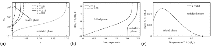
Figure 7: (a) Phase diagram of homopolymeric RNA in the $w$-$s$ plane for different values of the loop exponent $c=1.5,\,2.1,\,2.16,\,2.3$ featuring an unfolded phase (bottom right) and a folded phase (top left). For $c=c^{*}\approx 2.479$, the phase boundary approaches $s=1$ and the melting point $w_{\mathrm{c}}(s=1)$ diverges; therefore only the unfolded phase exists for $c\geq c^{*}$. For $c\leq 2$, there is no melting transition at zero force as $w_{\mathrm{c}}(s=1)=0$. Thus if no force is applied, the system is always in the folded phase regardless of the temperature. The molecule can be denatured, though, by applying an external force even for $c\leq 2$, as can be seen from the phase boundary for $c=1.5$. The filled circles denote the thermal denaturation transition point $w_{\mathrm{c}}(s=1)$ in the absence of an external force for $c=2.1,\,2.16,\,2.3$. (b) Phase diagram in the $w$-$c$ plane. With zero force, $s=1$ (solid line), the weight $w_{\mathrm{c}}$ drops to zero for $c\rightarrow 2$ and diverges as $c\rightarrow c^{*}\approx 2.479$. For finite force, $s>1$ (dashed line), a phase transition is possible, even for $c\leq 2$. (c) Phase diagram in the $F$-$T$ plane for $c=2.3$. Below the phase boundary the folded state is present, above the unfolded phase. Re-entrance at constant force is observed, as reported by Müller Mueller2003 .

In fig. 7b we show the critical line $w_{\mathrm{c}}(s,c)$ for two different values of $s$ as a function of the loop exponent $c$. In the absence of an external pulling force, i. e. for $s=1$ (solid line), the transition line only occurs in the limited range $2<c<c^{*}\approx 2.479$. It is seen that for loop exponents around the relevant value of $c\approx 2.1$, the critical base pairing weight is quite small and of the order of $w_{\mathrm{c}}\approx 0.1$. A base pairing weight smaller than unity corresponds to a repulsive base pairing free energy that is unfavorable. This at first sight paradoxical result, which means that the folded phase forms even when the extensive part of the base pairing free energy is repulsive, reflects the fact that the folded state contains a lot of topological entropy because of the degeneracy of different secondary structures. The consequences for the theoretical description of systems, where single stranded nucleic acids occur, including DNA transcription, denaturation bubbles in dsDNA, untwisting of nucleic acids Leger1999 , and translocation Bundschuh2005 will be briefly discussed in section 4.

The phase diagram, eq. (28), can also be displayed in the $F$-$T$ plane by virtue of eqs. (1) and (6) and is shown in fig. 7c. Here, re-entrance at constant force becomes visible, in line with previous predictions by Müller Mueller2003 . Expanding eq. (6) we obtain $s(F)\sim 1+(b_{\mathrm{ss}}F/(\mathrm{k_{B}}T))^{2}/6$, for $F\rightarrow 0$. Eq. (39) yields the scaling of the critical force close to the melting temperature as

$$F_{\mathrm{c}}\propto(T_{\mathrm{m}}-T)^{1/(2c-4)}\;,$$ (40)

which depends on the loop exponent $c$ and deviates from the predictions by Müller Mueller2003 , who found a universal exponent $1/2$.

3.3 Thermodynamic quantities and critical exponents

We now consider the thermodynamic and critical behavior of various quantities. An arbitrary extensive quantity $Y$ with the conjugate field $f$ is obtained from the grand potential $\Phi=-\mathrm{k_{B}}T\ln\mathcal{Z}$ via differentiation with respect to $f$ and the chemical potential $\mu$ held constant

$$Y=\left.\frac{\partial\Phi}{\partial f}\right|_{\mu}\;.$$ (41)

To evaluate the behavior of $Y$ in the thermodynamic limit, $N\rightarrow\infty$, one sets $\mu\rightarrow\mu_{\mathrm{d}}$, where $\mu_{\mathrm{d}}$ is defined as the chemical potential, at which $N(\mu)=-{\partial\Phi}/{\partial\mu}$ diverges, i. e. $N(\mu)\rightarrow\infty$ for $\mu\rightarrow\mu_{\mathrm{d}}$. Another route to obtain $Y$ is to conduct the calculation in the canonical ensemble, i. e. $N=\mathrm{const}$, and to use the dominating singularity Einert2010 , where

$$Y=\frac{\partial\mathcal{G}}{\partial f}=\mathrm{k_{B}}TN\frac{\partial\ln z_{\mathrm{d}}}{\partial f}\;,$$ (42)

see eq. (15). In fact, for $N\rightarrow\infty$ eqs. (41) and (42) are equivalent and $\mu_{\mathrm{d}}$ is associated with the dominating singularity of $\mathcal{Z}(z,s)$, namely $z_{\mathrm{d}}=\exp(\mu_{\mathrm{d}}/(\mathrm{k_{B}}T))$, which will be shown now. The Gibbs free energy $\mathcal{G}$ and the grand potential $\Phi$ are related via a Legendre transform

$$\mathcal{G}(N)=\Phi+\mu(N)N\;.$$ (43)

Therefore,

$$Y=\mathrm{k_{B}}TN\frac{\partial\ln z_{\mathrm{d}}}{\partial f}=\left.\frac{\partial\mathcal{G}}{\partial f}\right|_{N}=\left.\frac{\partial(\mathcal{G}-\Phi)}{\partial f}\right|_{N,\Phi}=N\left.\frac{\partial\mu}{\partial f}\right|_{\Phi}=\left.-\frac{\partial\Phi}{\partial\mu}\right|_{f}\left.\frac{\partial\mu}{\partial f}\right|_{\Phi}=\left.\frac{\partial\Phi}{\partial f}\right|_{\mu}\;,$$ (44)

where the two final expressions are evaluated at $\mu=\mu_{\mathrm{d}}$. While performing derivatives of the dominant singularity and of the function $\kappa(w,z)$ is straightforward for $z_{\mathrm{p}}$ and $\kappa_{\mathrm{p}}$, see eq. (22), one has to employ implicit differentiation of eq. (16) to obtain the derivative of $z_{\mathrm{b}}$ and $\kappa_{\mathrm{b}}$, see supplementary material. For the latter case it turns out that eq. (41) is more convenient to work with.

3.3.1 Fraction of paired bases

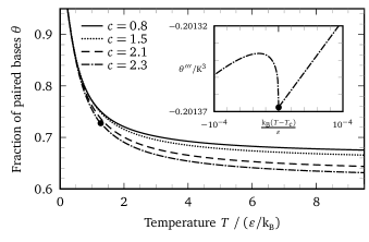
Figure 8: Fraction of paired bases as a function of temperature for $w=\exp(\varepsilon/(\mathrm{k_{B}}T))$ and various $c=0.8,\,1.5,\,2.1,\,2.3$ at zero force, $s=1$. A phase transition is observed only for $c=2.3$ for the range of positive values of $\varepsilon$ considered here (indicated by the filled circle), since for $c\lesssim 2.195$ the critical weight of a hydrogen bond is $w_{\mathrm{c}}<1$, which can only be obtained for $\varepsilon<0$ amounting to a repulsive interaction. For $c\leq 2$ no thermal phase transition can be observed at all. The inset shows the third derivative $\theta^{\prime\prime\prime}=\mathrm{d}^{3}\theta/\mathrm{d}T^{3}$ for $c=2.3$, which reveals the phase transition.

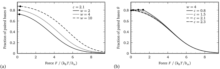
Figure 9: Fraction of paired bases as a function of force for various $w$ and $c$. The phase transition is visible as a kink in the curves and indicated by a filled circle. (a) $c=2.1$ and varying $w=2,\,4,\,10$. (b) $w=4$ and varying $c=0.8,\,1.5,\,2.1,\,2.3$.

The fraction of paired bases is

$$\theta=\frac{1}{N}\frac{\partial\ln Z_{N}}{\partial\ln w}\;.$$ (45)

We obtain

$$\theta=\frac{2\mathrm{Li}_{c}(z_{\mathrm{b}}\kappa(w,z_{\mathrm{b}}))}{\mathrm{Li}_{c-1}(z_{\mathrm{b}}\kappa(w,z_{\mathrm{b}}))}$$ (46)

in the folded phase ($T<T_{\mathrm{c}}$, $F<F_{\mathrm{c}}$) and

$$\theta=1-\frac{1}{\sqrt{1+4w\mathrm{Li}_{c}(1/s)}}$$ (47)

in the unfolded phase ($T>T_{\mathrm{c}}$, $F>F_{\mathrm{c}}$). In fig. 8 the temperature dependence and in fig. 9 the force dependence of $\theta$ is shown. The singularity at the critical point of the thermal phase transition for zero force, $s=1$, is very weak and becomes visible in the $n$^th derivative, with $n$ being the integer with $(c-2)^{-1}-1<n<(c-2)^{-1}$, see supplementary material. The $n$^th derivative exhibits a cusp, see inset of fig. 8,

$$\frac{\mathrm{d}^{n}\theta(T)}{\mathrm{d}T^{n}}\propto|T-T_{\mathrm{m}}|^{\lambda_{T}}+\mathrm{const}\;,$$ (48)

which is characterized by the critical exponent $\lambda_{T}=(c-2)^{-1}-n$ for $T<T_{\mathrm{m}}$ and $\lambda_{T}=1$ for $T>T_{\mathrm{m}}$, see supplementary material. The force induced phase transition is continuous, too, yet it exhibits a kink in $\theta(F)$

$$\theta(F)\propto|F-F_{\mathrm{c}}|^{\lambda_{F}}+\mathrm{const}\;,$$ (49)

which is characterized by the exponents $\lambda_{F}=0$ for $F<F_{\mathrm{c}}$ and $\lambda_{F}=1$ for $F>F_{\mathrm{c}}$. Therefore, the force induced phase transition is second order in accordance with previous results Mueller2003 ; Montanari2001 . We note that for $T\rightarrow\infty$, i. e. $w\rightarrow 1$, a finite fraction of bases are still paired. The situation is different for the force induced phase transition where $\theta\rightarrow 0$ for $F\rightarrow\infty$.

3.3.2 Specific heat

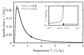
Figure 10: Specific heat as a function of temperature for different loop exponents $c=0.8,\,2.3$. The non-critical behavior of the heat capacity curve depends on the loop exponent only marginally. However, the existence and position of the critical point (indicated by the filled circle) and the critical behavior depend on $c$. The inset depicts the third derivative of the specific heat, $C^{\prime\prime\prime}=\mathrm{d}^{3}C/\mathrm{d}T^{3}$, for $c=2.3$ revealing the phase transition.

The specific heat is defined as

$$C=\frac{\mathrm{k_{B}}T}{N}\frac{\partial^{2}T\ln Z_{N}}{\partial T^{2}}\;.$$ (50)

One observes that the specific heat in fig. 10 exhibits only a very weak dependence on the loop exponent, which stands in marked contrast to the findings for the short explicit sequence of tRNA-phe Einert2008 ; Einert2010a , where a pronounced dependence of the heat capacity on $c$ is observed. The non-analyticity of $\theta$, eq. (48), translates into a divergence of the $n$^th derivative of the specific heat at the melting temperature

$$\frac{\mathrm{d}^{n}C(T)}{\mathrm{d}T^{n}}\propto|T-T_{\mathrm{m}}|^{-\chi}+\mathrm{const}\;,$$ (51)

with the critical exponent $\chi=n-(3-c)/(c-2)$ for $T<T_{\mathrm{m}}$ and $\chi=1$ for $T>T_{\mathrm{m}}$. This singularity is illustrated in the inset of fig. 10 for $c=2.3$.

3.3.3 Fraction of non-nested backbone bonds

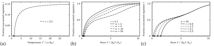
Figure 11: (a) Fraction of non-nested backbone bonds $\tau$ as a function of temperature for $c=2.3$. For $c\lesssim 2.195$ the critical weight of a hydrogen bond is $w_{\mathrm{c}}<1$, which can only be obtained for $\varepsilon<0$, amounting to a repulsive interaction. Thus, for $c\lesssim 2.195$ or $T<T_{\mathrm{m}}$ all segments are parts of loops or helices and hence $\tau=0$. Filled circles indicate the melting temperature $T_{\mathrm{m}}$. (b) and (c) fraction of non-nested backbone bonds as a function of force for various $w$ and $c$. Again, the phase transition is visible as a kink in the curves and is indicated by a filled circle. (b) $c=2.1$ and varying $w=2,\,4,\,10,\,50$. (c) $w=50$ and varying $c=0.8,\,1.5,\,2.1,\,2.3$. Filled circles indicate the position of the phase transition.

The fraction of non-nested backbone bonds is obtained by

$$\tau=\frac{1}{N}\frac{\partial\ln Z_{N}}{\partial\ln s}$$ (52)

and is

$$\tau=0$$ (53)

in the folded phase, as $z_{\mathrm{b}}$ does not depend on $s$, and reads

$$\tau=1-\frac{2w\mathrm{Li}_{c-1}(1/s)}{1+4w\mathrm{Li}_{c}(1/s)+\sqrt{1+4w\mathrm{Li}_{c}(1/s)}}$$ (54)

in the unfolded phase. For $T\rightarrow\infty$ the fraction of non-nested backbone bonds assumes a finite value smaller than one, which again indicates that the denatured phase in our model features pronounced base pairing. However, for large force $F\rightarrow\infty$ on invariably obtains $\tau\rightarrow 1$. As can be seen nicely in fig. 11, both $\tau({T})$ and $\tau({F})$ feature a kink at the critical point.

3.3.4 Force extension curve

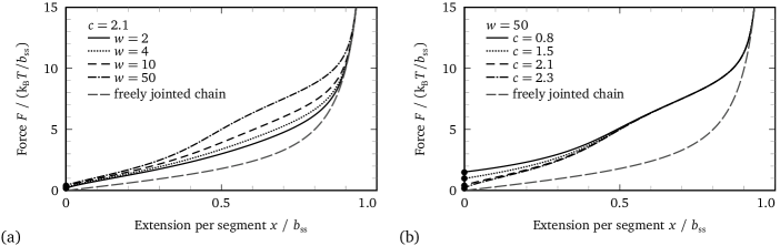
Figure 12: Force extension curve as a function of force for various $w$ and $c$. The phase transition is indicated by filled circles and occurs at zero extension and a finite threshold force needed to unfold the compact folded structure. (a) $c=2.1$ and varying $w=\exp(\varepsilon/\mathrm{k_{B}}T)=2,\,4,\,10,\,50$. (b) $w=50$ and varying $c=0.8,\,1.5,\,2.1,\,2.3$. Additionally the force extension curve of a freely jointed chain is plotted, which is the limiting form for $w=0$.

The force extension curve is closely related to the fraction of non-nested backbone bonds $\tau$. The extension per monomer is given by

$$x(F)=\frac{\mathrm{k_{B}}T}{N}\frac{\partial\ln Z_{N}}{\partial F}=\frac{\mathrm{k_{B}}T}{N}\frac{\partial\ln Z_{N}}{\partial\ln s}\frac{\partial\ln s}{\partial F}=b_{\mathrm{ss}}\tau\ (\coth(\beta Fb_{\mathrm{ss}})-1/(\beta Fb_{\mathrm{ss}}))=b_{\mathrm{ss}}\tau\ \mathcal{L}(\beta Fb_{\mathrm{ss}})\;,$$ (55)

Since the Langevin function $\mathcal{L}$ is a smooth function, the critical behavior of $x(F)$ is governed by the behavior of the fraction of non-nested bonds $\tau$. As can be seen in fig. 12a, the stretching behavior of the Langevin function is approached as the base pairing weight decreases, otherwise pronounced deviations are seen in the force-stretching curves. Also, a finite stretching force to unravel the folded state is needed. From fig. 12 it becomes obvious that the force induced phase transition is second order as the force extension curve exhibits a kink at the critical force denoted by filled circles. The force extension curves are in accordance with previous results Montanari2001 ; Mueller2003 .

4 Implications for DNA melting

How do the previous results impact on the theoretical description of the denaturation of double stranded nucleic acid systems, particularly DNA melting? When double stranded DNA approaches the denaturation transition, more and more inter-strand base pairs break up and loops proliferate. In the traditional theories based on the Poland-Scheraga model Poland1966 ; Poland1966a , the possibility of intra-strand base pairing was not considered. These models are thus accurate for duplexes formed between strands with sequences $[\mathrm{AG}]_{N/2}$ and $[\mathrm{TC}]_{N/2}$, where indeed base pairs (between A and T and between G and C) can only form between the two strands, not within one strand. For the case of duplexes formed by two strands with the sequence $[\mathrm{AT}]_{N/2}$ or $[\mathrm{GC}]_{N/2}$, both intra- and inter-strand base pairs can form and have identical statistical weights. In this case, our model predicts significant modifications for the duplex melting scenario.

The above sequence examples are prototypes for two extreme cases of the general scenario characterized by statistical weights $w$ and $\hat{w}$ for intra-strand and inter-strand pairing, respectively. Duplexes formed between $[\mathrm{AG}]_{N/2}$ and $[\mathrm{TC}]_{N/2}$ are characterized by $w=0$, whereas duplexes formed between two $[\mathrm{AT}]_{N/2}$ or $[\mathrm{CG}]_{N/2}$ strands are characterized by $w=\hat{w}$. Intermediate values of $w$ and $\hat{w}$ can be achieved experimentally, for example, by $[\mathrm{ATT}]_{N/3}$ and its complementary sequence $[\mathrm{AAT}]_{N/3}$, in which case only $2/3$ of the intra-strand base pairs can be of the Watson-Crick type and which would effectively lead to a lower weight of intra-strand base pairs, i. e. $w<\hat{w}$. In naturally occurring DNA, a similar situation might be present above the glass transition where, for certain sequences, self-hybridization in a single strand is possible to some extent Bundschuh2002a . The weights of inter-strand and intra-strand base pairs can also be changed by applying an external force or torque on the duplex, for instance in the setup by Léger et al. Leger1999 . We expect the weight $\hat{w}$ of inter-strand base pairs to decrease when the duplex is untwisted. This might lead to denatured regions in the duplex, where secondary structure can form if the sequence allows. We speculate that subsequent pulling first leads to the denaturation of the secondary structures, whose signature would be a threshold force around $1\text{\,}\mathrm{pN}$-$10\text{\,}\mathrm{pN}$ Montanari2001 ; Einert2010a , see fig. 12, followed by the over-stretching transition of DNA Einert2010 . According to our previous arguments, a marked dependence on the sequence should be observed.

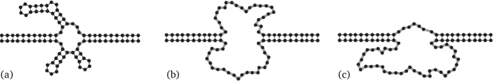
Figure 13: Illustration of a double stranded DNA molecule near the melting transition. (a) If intra-strand base pairing is possible, in inter-strand loops the vast majority of bases will form intra-strand secondary structure elements. (b) If the sequence does not favor intra-strand base pairs inter-strand loops without secondary structure will form. (c) Illustration of an asymmetric loop.

Let us now review the classical Poland-Scheraga calculation Poland1966 ; Poland1966a and allow – in addition to the standard treatment – for intra-strand base pairing in denatured regions of the duplex, see fig. 13a. The grand canonical partition function of the two-state Poland-Scheraga model reads

$$\hat{{\mathcal{Z}}}=(1+\hat{{\mathcal{Z}}}_{\mathrm{M}})\sum_{k=0}^{\infty}(\hat{{\mathcal{Z}}}_{\mathrm{B}}\hat{{\mathcal{Z}}}_{\mathrm{M}})^{k}(1+\hat{{\mathcal{Z}}}_{\mathrm{B}})-1=\frac{\hat{{\mathcal{Z}}}_{\mathrm{B}}+\hat{{\mathcal{Z}}}_{\mathrm{M}}+2\hat{{\mathcal{Z}}}_{\mathrm{B}}\hat{{\mathcal{Z}}}_{\mathrm{M}}}{1-\hat{{\mathcal{Z}}}_{\mathrm{B}}\hat{{\mathcal{Z}}}_{\mathrm{M}}}\;,$$ (56)

where

$$\hat{{\mathcal{Z}}}_{\mathrm{B}}=\sum_{N=1}^{\infty}(z\hat{w})^{N}=\frac{z\hat{w}}{1-z\hat{w}}$$ (57)

is the grand canonical partition function of a duplex in the bound state with $\hat{w}$ the weight of an inter-strand base pair and $z$ now plays the role of the fugacity of a base pair. We distinguish between three different scenarios for a denatured or molten region inside the double strand, which is characterized by the partition function $\hat{{\mathcal{Z}}}_{\mathrm{M}}$, depending on the sequence and the intra-strand base pairing weight $w$: (i) for $w>w_{\mathrm{c}}$, with $w_{\mathrm{c}}$ defined by eq. (28), intra-strand secondary structures in the folded (low temperature) phase are present, (ii) for $w<w_{\mathrm{c}}$ intra-strand secondary structures in the unfolded (high temperature) phase form, and (iii) for $w=0$ large denaturation bubbles occur without intra-strand base pairing, corresponding to the original Poland-Scheraga model. The grand canonical partition for case (i) is characterized by the branch point singularity, eq. (20),

$$\hat{{\mathcal{Z}}}_{\mathrm{M}}^{\mathrm{i}}=\sum_{N=1}^{\infty}z^{N}\bigl{(}z_{\mathrm{b}}^{-N}N^{-3/2}\bigr{)}^{2}=\mathrm{Li}_{{\hat{c}_{\mathrm{eff}}}}(z/z_{\mathrm{b}}^{2})\;,$$ (58)

with ${\hat{c}_{\mathrm{eff}}}=3$ and where the square is due to the fact, that on either strand secondary structures may form; $N$-independent factors have been neglected as they do not affect the critical behavior. One realizes that the effective loop exponent ${\hat{c}_{\mathrm{eff}}}$ in this case is universal and independent of the configurational entropy of an inter-strand loop characterized by the exponent ${\hat{c}}$. For case (ii), the secondary structures on each strand are in the unfolded phase and the partition functions are characterized by the pole, eq. (26). As the number of non-nested segments, which is proportional to $N$, is non-zero, eq. (54), an inter-strand loop decorated with helices occurs, and is characterized by the loop exponent ${\hat{c}}$. The respective grand canonical partition function reads

$$\hat{{\mathcal{Z}}}_{\mathrm{M}}^{\mathrm{ii}}=\sum_{N=1}^{\infty}z^{N}\bigl{(}z_{\mathrm{p}}^{-N}\bigr{)}^{2}N^{-{\hat{c}}}=\mathrm{Li}_{{\hat{c}}}(z/z_{\mathrm{p}}^{2})\;.$$ (59)

The third case constitutes the classical Poland-Scheraga model, where no base pairing is present and the loop exponent ${\hat{c}}$ describes the loop statistics. The partition function reads

$$\hat{{\mathcal{Z}}}_{\mathrm{M}}^{\mathrm{iii}}=\sum_{N=1}^{\infty}z^{N}N^{-{\hat{c}}}=\mathrm{Li}_{{\hat{c}}}(z)\;.$$ (60)

Combining eqs. (56-60) yields the grand canonical partition function of a nucleic acid duplex

$$\hat{{\mathcal{Z}}}=\frac{\hat{w}z+(1+\hat{w}z)\mathrm{Li}_{{\hat{c}_{\mathrm{eff}}}}(z/\hat{z}_{\mathrm{b}})}{1-\hat{w}z(1+\mathrm{Li}_{{\hat{c}_{\mathrm{eff}}}}(z/\hat{z}_{\mathrm{b}}))}\;,$$ (61)

with (i) ${\hat{c}_{\mathrm{eff}}}=3$, $\hat{z}_{\mathrm{b}}=z_{\mathrm{b}}^{2}$, (ii) ${\hat{c}_{\mathrm{eff}}}={\hat{c}}=2.1$, $\hat{z}_{\mathrm{b}}=z_{\mathrm{p}}^{2}$, or (iii) ${\hat{c}_{\mathrm{eff}}}={\hat{c}}=2.1$, $\hat{z}_{\mathrm{b}}=1$, respectively.

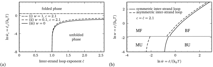
Figure 14: (a) The critical inter-strand binding energy $\ln\hat{w}_{\mathrm{c}}$ as a function of the inter-strand loop exponent ${\hat{c}}$ for different intra-strand base pairing weights $w$ and different intra-strand loop exponents $c$. (i) for $w>w_{\mathrm{c}}$, with $w_{\mathrm{c}}(c=2.1)\approx 0.16$, see eq. (28), inside denatured regions of the duplex secondary structures that are folded occur on each strand. (ii) for $w<w_{\mathrm{c}}$ secondary structures that are unfolded form on each strand. (iii) for $w=0$ the classical Poland-Scheraga result is obtained, where no intra-strand base pairs form. (b) Phase diagram of a nucleic acid duplex in the plane spanned by the intra-strand pairing weight $w$ and the inter-strand pairing weight $\hat{w}$ for symmetric (solid line) and asymmetric (dashed line) inter-strand loops for $c={\hat{c}}=2.1$. Left to these curves the duplex is in the molten (M) phase, to the right the duplex is in the bound (B) phase. The dotted line at $w=w_{\mathrm{c}}(c=2.1)\approx 0.16$, see eq. (28), depicts the phase boundary between folded (F) and unfolded (U) intra-strand secondary structures for $c=2.1$, which separates cases (i) and (ii), respectively.

The thermodynamics of nucleic acid duplexes is governed by the singularities of the partition function, eq. (61). The singularities are readily recognized as the branch point $\hat{z}_{\mathrm{b}}$ of the polylogarithm Abramowitz2002 and the pole $\hat{z}_{\mathrm{p}}$ of the fraction in eq. (61), which is the root of the denominator

$$1=\hat{w}\hat{z}_{\mathrm{p}}(1+\mathrm{Li}_{{\hat{c}_{\mathrm{eff}}}}(\hat{z}_{\mathrm{p}}/\hat{z}_{\mathrm{b}}))\;.$$ (62)

At the critical point, the pole and the branch point coincide, $\hat{z}_{\mathrm{b}}=\hat{z}_{\mathrm{p}}$, which yields

$$\hat{w}_{\mathrm{c}}=\frac{1}{\hat{z}_{\mathrm{b}}\bigl{(}1+\zeta_{{\hat{c}_{\mathrm{eff}}}}\bigr{)}}\;,$$ (63)

where $\zeta_{{\hat{c}_{\mathrm{eff}}}}=\mathrm{Li}_{{\hat{c}_{\mathrm{eff}}}}(1)$ is the Riemann zeta function. In fig. 14a the critical inter-strand base pairing weight $\hat{w}_{\mathrm{c}}$ as a function of the inter-strand loop exponent ${\hat{c}}$ is shown. The solid line depicts the phase diagram of the classical Poland-Scheraga model (iii) characterized by $w=0$, where no secondary structures occur in denatured regions, cf. fig. 13b. The dashed line depicts the phase diagram for $w=0.1$, where secondary structures occur that are in the unfolded state since $w=0.1<w_{\mathrm{c}}$ for $c=2.1$, (ii). One sees that the modifications to the $w=0$ limit are rather small. As in the case of the classical Poland-Scheraga model there is no phase transition for ${\hat{c}}\leq 1$, a second order phase transition for $1<{\hat{c}}\leq 2$, and a first order transition for ${\hat{c}}>2$ Poland1966 ; Poland1966a ; Kafri2000 . The situation is different for case (i) with $w=1$, where the secondary structures are in the folded and the inter-strand loop exponent is replaced by the universal value ${\hat{c}_{\mathrm{eff}}}=3$, which renders the denaturation transition first order and independent of ${\hat{c}}$. In fig. 14b the phase boundary in the $w$-$\hat{w}$ plane is shown. The phase boundaries arising due to inter-strand base pairing (solid or dashed line) and intra-strand base pairing (dotted line) section the phase space into four quadrants, where the duplex is either in the bound (B) or molten (M) state and the intra-strand secondary structures are either folded (F, case (i)) or unfolded (U, case (ii)). Experimentally, a variation of temperature corresponds to a straight path through the origin of the phase diagram in fig. 14b, which, depending on the values of the inter- and intra-strand energies $\hat{\varepsilon}$ and $\varepsilon$, may cross a number of different phases.

There are $2N$ ways of constructing an asymmetric inter-strand loop Garel2004 , where the number of bases in the lower and the upper part of a loop is not required to be identical, see fig. 13c for an illustration. This additional factor reduces the inter-strand loop exponent ${\hat{c}}$ by $1$. Therefore, the duplex denaturation transition is for case (i) right at the threshold between continuous and discontinuous transitions, because ${\hat{c}_{\mathrm{eff}}}=2$, and for cases (ii,iii) a continuous transition as ${\hat{c}_{\mathrm{eff}}}=1.1$. The consequences on the phase behavior are illustrated in fig. 14b by broken lines. We add that the results for the competition between intra- and inter-strand base pairing are obtained using a factorization approximation for the two strands making up an inter-strand loop. In the appendix we show that this factorization is accurate in the thermodynamic limit of diverging loop size.

As a main result, the effective inter-strand loop exponent is renormalized and takes on universal values for case (i), where intra-strand base pairing leads to secondary structures in the folded phase. The formation of intra-strand secondary structure influences the melting temperature and has implications for the determination base pairing free energy parameters SantaLucia1998 ; Xia1998 and other biotechnological applications where DNA melting and hybridization is involved. Thus, intra-strand interaction might be important to include in software packages predicting the stability of nucleic acids based on a Poland-Scheraga scheme. Algorithms for cofolding of multiple nucleic acids already account for this Hofacker2003 ; Markham2005 ; Schuster2006 .

5 Conclusions

The partition function of RNA secondary structures has been evaluated including arbitrary pairing topologies in the absence of pseudoknots, including the configurational entropy of loops in the form of the loop length dependent term $\mathcal{G}_{\mathrm{l}}^{\mathrm{conf}}=-\mathrm{k_{B}}T\ln m^{-c}$. Exact expressions for the fraction of paired bases, the heat capacity, and the force extension curves are derived in the presence of an external pulling force. The observed thermal phase transition is very weak and of higher order, the force induced transition is found to be second order. The critical behavior and the critical exponents are found to depend on the loop exponent $c$. A temperature induced melting transition is only possible for $2<c<c^{*}\approx 2.479$. Our theory has consequences on the denaturation of double stranded DNA molecules, in particular when intra-strand base pairs as well as inter-strand base pairs can form. In this case, the native double strand is in competition with intra-strand base pairing effecting the secondary structures discussed in this paper. Future directions will include loop exponents, that depend on the number of helices emerging from a given loop, treatment of pseudoknots, and cofolding nucleic acids to study the influence of intra-strand interactions during double strand denaturation.

Appendix A Appendix

The statistical weight of a $N$ base pair long molten region in the duplex with intra-strand interaction, as depicted in fig. 13a, is given by

$$Z^{\mathrm{DNA}}_{N}=\sum_{M,M^{\prime}=0}^{N}s^{M+M^{\prime}+4}\frac{\tilde{Q}_{N}^{M}\tilde{Q}_{N}^{M^{\prime}}}{(M+M^{\prime}+4)^{{\hat{c}}}}\;,$$ (64)

where ${\hat{c}}=2.1$ is the loop exponent describing inter-strand loops in DNA, $M+M^{\prime}+4$ counts the number of non-nested back-bones that contribute to the loop entropy, and $\tilde{Q}_{N}^{M}$ is given by eq. (4). The denominator in eq. (64) is due to the loop entropy and amounts to an effective interaction between the two strands as the expectation value of $M$ depends on $M^{\prime}$ and vice versa. The asymptotic behavior of $Z^{\mathrm{DNA}}_{N}$ can be estimated by establishing two inequalities. The first is

$$Z^{\mathrm{DNA}}_{N}\leq s^{4}\sum_{M=0}^{N}s^{M}\tilde{Q}_{N}^{M}\sum_{M^{\prime}=0}^{N}s^{M^{\prime}}\tilde{Q}_{N}^{M^{\prime}}=s^{4}Z_{N}Z_{N}\;,$$ (65)

where the scaling of $Z_{N}$ is given by eq. (20) or (26) depending on whether the secondary structures are in the folded or unfolded phase, respectively. The upper scaling boundary is obtained by factorizing eq. (64) and therefore removing the effective interaction, but retaining the loop entropy for each individual strand

$$Z^{\mathrm{DNA}}_{N}\geq\sum_{M=0}^{N}\frac{s^{M+2}\tilde{Q}_{N}^{M}}{(M+2)^{{\hat{c}}}}\sum_{M^{\prime}=0}^{N}\frac{s^{M^{\prime}+2}\tilde{Q}_{N}^{M^{\prime}}}{(M^{\prime}+2)^{{\hat{c}}}}\;.$$ (66)

The scaling of eq. (66) follows from the dominant singularity analysis of the generating function

$$\mathcal{Z}^{\sqrt{\mathrm{DNA}}}(z,s)=s^{2}z^{2}\sum_{N=0}^{\infty}\sum_{M=0}^{N}s^{M}z^{N}\frac{\tilde{Q}_{N}^{M}}{(M+2)^{{\hat{c}}}}=\frac{1}{\kappa(w,z)}\mathrm{Li}_{{\hat{c}}}(sz\kappa(w,z))-sz\;.$$ (67)

$\mathcal{Z}^{\sqrt{\mathrm{DNA}}}(z,s)$ features the same singularities as $\mathcal{Z}(z,s)$, see eq. (9), namely the branch point of $z_{\mathrm{b}}$ of $\kappa(w,z)$, and the singularity $z_{\mathrm{p}}$ given by the condition $1=sz\kappa(w,z)$, see eq. (22).

By virtue of the inequalities (65) and (66) we conclude that

$$Z^{\mathrm{DNA}}_{N}\propto\hat{z}_{\mathrm{b}}^{-N}N^{-{\hat{c}_{\mathrm{eff}}}}\;$$ (68)

with ${\hat{c}_{\mathrm{eff}}}=3$, $\hat{z}_{\mathrm{b}}=z_{\mathrm{b}}^{2}$ for case (i) and ${\hat{c}_{\mathrm{eff}}}={\hat{c}}=2.1$, $\hat{z}_{\mathrm{b}}=z_{\mathrm{p}}^{2}$ for case (ii) for symmetric molten loops.

See pages - of RNA_homo_supplementary_material.pdf

References

- (1) R.F. Gesteland, T.R. Cech, J.F. Atkins, eds., The RNA World, 2nd edn. (Cold Spring Harbor Laboratory Press, Woodbury, 2005)
- (2) S.B. Smith, Y.J. Cui, C. Bustamante, Science 271(5250), 795 (1996)
- (3) J. Liphardt, S. Dumont, S.B. Smith, J. Tinoco, Ignacio, C. Bustamante, Science 296(5574), 1832 (2002)
- (4) M. Rief, H. Clausen-Schaumann, H.E. Gaub, Nat. Struct. Biol. 6(4), 346 (1999)
- (5) B. Maier, D. Bensimon, V. Croquette, Proc. Natl. Acad. Sci. U. S. A. 97(22), 12002 (2000)
- (6) U. Bockelmann, B. Essevaz-Roulet, F. Heslot, Phys. Rev. Lett. 79(22), 4489 (1997)
- (7) A. Mossa, M. Manosas, N. Forns, J.M. Huguet, F. Ritort, J. Stat. Mech. 2009, P02060 (2009)
- (8) I. Tinoco, O.C. Uhlenbeck, M.D. Levine, Nature 230, 362 (1971)
- (9) I. Tinoco, Jr, C. Bustamante, J. Mol. Biol. 293(2), 271 (1999)
- (10) A.V. Finkelstein, O.V. Galzitskaya, Phys. Life Rev. 1(1), 23 (2004), ISSN 1571-0645
- (11) P.G. de Gennes, Biopolymers 6(5), 715 (1968)
- (12) M.S. Waterman, T.F. Smith, Math. Biosci. 42, 257 (1978)
- (13) T.R. Einert, P. Näger, H. Orland, R.R. Netz, Phys. Rev. Lett. 101(4), 048103 (2008)
- (14) I.L. Hofacker, W. Fontana, P.F. Stadler, L.S. Bonhoeffer, M. Tacker, P. Schuster, Mon. Chem. 125(2), 167 (1994)
- (15) J.S. McCaskill, Biopolymers 29, 1105 (1990)
- (16) T.R. Einert, D.B. Staple, H. Kreuzer, R.R. Netz, Biophys. J. 99(2), 578 (2010)
- (17) A. Montanari, M. Mézard, Phys. Rev. Lett. 86, 2178 (2001)
- (18) U. Gerland, R. Bundschuh, T. Hwa, Biophys. J. 81(3), 1324 (2001)
- (19) M. Müller, F. Krzakala, M. Mézard, Eur. Phys. J. E 9, 67 (2002)
- (20) A. Hanke, M.G. Ochoa, R. Metzler, Phys. Rev. Lett. 100(1), 018106 (2008)
- (21) S. Cocco, J.F. Marko, R. Monasson, C. R. Phys. 3(5), 569 (2002)
- (22) D.K. Lubensky, D.R. Nelson, Phys. Rev. E 65, 031917 (2002)
- (23) R. Bundschuh, U. Gerland, Phys. Rev. Lett. 95, 208104 (2005)
- (24) T.R. Einert, R.R. Netz (2010), to be published
- (25) Z.J. Tan, S.J. Chen, Biophys. J. 90(4), 1175 (2006)
- (26) Y.S. Mamasakhlisov, S. Hayryan, V.F. Morozov, C.K. Hu, Phys. Rev. E 75(6), 061907 (2007)
- (27) M. Baiesi, E. Orlandini, A.L. Stella, Phys. Rev. Lett. 91(19), 198102 (2003)
- (28) H. Orland, A. Zee, Nucl. Phys. B 620(3), 456 (2002)
- (29) R. Blossey, E. Carlon, Phys. Rev. E 68(6), 061911 (2003)
- (30) Y. Kafri, D. Mukamel, L. Peliti, Phys. Rev. Lett. 85(23), 4988 (2000)
- (31) B. Alberts, Molecular Biology of the Cell (Garland Science, 2002)
- (32) J.C.M. Gebhardt, T. Bornschlögl, M. Rief, Proc. Natl. Acad. Sci. U. S. A. 107(5), 2013 (2010)
- (33) T. Xia, J. SantaLucia, Jr, M.E. Burkard, R. Kierzek, S.J. Schroeder, X. Jiao, C. Cox, D.H. Turner, Biochemistry 37(42), 14719 (1998)
- (34) R. Bundschuh, T. Hwa, Europhys. Lett. 59(6), 903 (2002)
- (35) P.G. de Gennes, Scaling Concepts in Polymer Physics (Cornell University Press, 1979)
- (36) B. Duplantier, Phys. Rev. Lett. 57(8), 941 (1986)
- (37) M. Müller, Phys. Rev. E 67(2), 021914 (2003)
- (38) A. Erdélyi, Higher Transcendental Functions, Vol. 1 (McGraw-Hill, 1953)
- (39) P. Flajolet, A. Odlyzko, SIAM Discret. Math. 3(2), 216 (1990)
- (40) M. Abramowitz, I.A. Stegun, eds., Handbook of Mathematical Functions, tenth edn. (U.S. Department of Commerce, 2002)
- (41) J.F. Léger, G. Romano, A. Sarkar, J. Robert, L. Bourdieu, D. Chatenay, J.F. Marko, Phys. Rev. Lett. 83(5), 1066 (1999)
- (42) D. Poland, H.A. Scheraga, J. Chem. Phys. 45(5), 1456 (1966)
- (43) D. Poland, H.A. Scheraga, J. Chem. Phys. 45(5), 1464 (1966)
- (44) T. Garel, H. Orland, Biopolymers 75(6), 453 (2004)
- (45) J. SantaLucia, Jr., Proc. Natl. Acad. Sci. U. S. A. 95(4), 1460 (1998)
- (46) I.L. Hofacker, Nucleic Acids Res. 31(13), 3429 (2003)
- (47) N.R. Markham, M. Zuker, Nucleic Acids Res. 33, W577 (2005)
- (48) P. Schuster, Rep. Prog. Phys. 69, 1419 (2006)