On the Origin of Model Relations among Transverse-Momentum Dependent Parton Distributions

Abstract

Transverse-momentum dependent parton distributions (TMDs) are studied in the framework of quark models. In particular, quark-model relations among TMDs are reviewed, elucidating their physical origin in terms of the quark-spin structure in the nucleon. The formal aspects of the derivation of these relations are complemented with explicit examples, emphasizing how and to which extent the conditions which lead to relations among TMDs are implemented in different classes of quark models.

I Introduction

Transverse-momentum dependent parton distributions (TMDs) have received a great attention in the last years as they represent key objects to map out the three-dimensional partonic structure of hadrons in momentum space. The dependence on the transverse momentum of the quark allows for a full account of the orbital motion of the quarks and introduces non-trivial correlations between the orbital angular momentum and the spin of the quark inside nucleons with different polarization states. TMDs typically give rise to spin and azimuthal asymmetries in, for instance, semi-inclusive deep inelastic scattering and Drell-Yan processes, and significant efforts have already been devoted to measure these observables (see, e.g., Ref. Barone:2010zz for a recent review). However, the extraction of TMDs from experimental data is a quite difficult task and needs educated Ansätze for fits of TMD parametrizations. To this aim, model calculations of TMDs play a crucial role and are essential towards an understanding of the non-perturbative aspects of TMDs. At leading twist there are eight TMDs, three of them surviving when integrated over the transverse momentum and giving rise to the familiar parton density, helicity and transversity distributions. Studies of the TMDs have been mainly focused on the quark contribution, and predictions have been obtained within a variety of models Jakob:1997wg ; Goldstein:2002vv ; Pobylitsa:2002fr ; Gamberg:2003ey ; Lu:2004au ; Cherednikov:2006zn ; Lu:2006kt ; Gamberg:2007wm ; Pasquini:2009bv ; Efremov:2009ze ; She:2009jq ; Zhu:2011zza ; Lu:2010dt ; Avakian:2009jt ; Courtoy:2008dn ; Courtoy:2009pc ; Courtoy:2008vi ; Pasquini:2010af ; Brodsky:2010vs ; Lorce:2007fa ; Pasquini:2008ax ; Boffi:2009sh ; Pasquini:2010pa ; Lorce:2011dv ; Bacchetta:2008af ; Avakian:2010br ; Avakian:2008dz ; Efremov:2010mt ; Meissner:2007rx ; Wakamatsu:2009fn ; Schweitzer:2001sr . Despite the specific assumptions for modeling the quark dynamics, most of these models predicted relations among the leading-twist TMDs. Since in QCD the eight TMDs are all independent, it is clear that such relations should be traced back to some common simplifying assumptions in the models. First of all, it was noticed that they break down in models with gauge-field degrees of freedom. Furthermore, most quark models are valid at some very low scale and these relations are expected to break under QCD evolution to higher scales. Despite these limitations, such relations are intriguing because they can provide guidelines for building parametrizations of TMDs to be tested with experimental data and also can give useful insights for the understanding of the origin of the different spin-orbit correlations of quarks in the nucleon.

The aim of this paper is to review these model relations and in particular to explain their physical origin. In Sec. II we give the formalism for the definition of the leading-twist TMDs, and introduce a convenient representation of the quark-quark correlator in terms of the net polarization states of the quark and hadrons. The model relations among TMDs are introduced and explained in details in Sec. III. In particular, there are two linear relations and a quadratic relation which are flavor independent and involve polarized TMDs, while a further linear relation is flavor dependent and involves both polarized and unpolarized TMDs.

The relations among polarized TMDs connect the distributions of quarks inside the nucleon for different configurations of the polarization states of the hadron and the partons. As a consequence, it is natural to expect that they can originate from rotational invariance of the polarization states of the system. Rotations are more easily discussed in the basis of canonical spin. Therefore, instead of working in the standard basis of light-cone helicity, we introduce in Secs. IV-A and IV-B the tensor correlator defining the TMDs in the canonical-spin basis. Such a representation is used in Sec. IV-C to discuss the consequences of rotational symmetries of the system. In such a way we will be able to identify the key ingredients for the existence of relations among polarized TMDs in quark models.
In order to complete the discussion, including the flavor-dependent relation among polarized and unpolarized TMDs, we need to introduce specific assumptions about the spin-isospin structure of the nucleon state. Therefore, in Sec. V we discuss the consequences of rotational invariance using the explicit representation of the TMDs in terms of three-quark (3Q) wave functions. In particular, in Sec. V-A we derive the overlap representation of the TMDs in terms of light-cone wave functions, while the corresponding representation in terms of wave function in the canonical-spin basis is given in Sec. V-B. In Sec. V-C we discuss the constraints of rotational symmetry on the nucleon wave function and, as a result, we give an alternative derivation of the flavor-independent relations among TMDs. Finally, in Sec. V-D we discuss the constraint due to $SU(6)$ symmetry of the spin-flavor dependent part of the nucleon wave function. This additional ingredient allows us to explain the origin of the flavor-dependent relation.

The formal derivation of the relations among TMDs is made explicit within different quark models in the final Sec. VI. There we review different quark models which have been used in literature for the calculation of TMDs. In particular, we discuss the key ingredients of the models, showing how and to which extent the conditions which lead to relations among TMDs are realized. A summary of our findings is given in the final section. Technical details and further explanations about the representation in terms of nucleon wave functions are collected in three appendices.

II Transverse-Momentum Dependent Parton Distributions

II.1 Definitions

In this section, we review the formalism for the definition of TMDs, following the conventions of Refs. Mulders:1995dh ; Boer:1997nt ; Goeke:2005hb . Introducing two lightlike four-vectors $n_{\pm}$ satisfying $n_{+}\cdot n_{-}=1$, we write the light-cone components of a generic four-vector $a$ as $\left[a^{+},a^{-},\boldsymbol{a}_{\perp}\right]$ with $a^{\pm}=a\cdot n_{\mp}$.
The density of quarks can be defined from the following quark-quark correlator

$$\Phi_{ab}(x,\boldsymbol{k}_{\perp},S)=\int\frac{\mathrm{d}\xi^{-}\,\mathrm{d}^{2}\xi_{\perp}}{(2\pi)^{3}}\,e^{i\left(k^{+}\xi^{-}-\boldsymbol{k}_{\perp}\cdot\boldsymbol{\xi}_{\perp}\right)}\langle P,S|\overline{\psi}_{b}(0)\mathcal{U}^{n_{-}}_{(0,+\infty)}\mathcal{U}^{n_{-}}_{(+\infty,\xi)}\psi_{a}(\xi)|P,S\rangle\big{|}_{\xi^{+}=0},$$ (1)

where $k^{+}=xP^{+}$, $\psi$ is the quark field operator with $a,b$ indices in the Dirac space, and $\mathcal{U}$ is the Wilson line which ensures color gauge invariance Bomhof:2004aw . The target state is characterized by its four-momentum $P$ and covariant spin four-vector $S$ satisfying $P^{2}=M^{2}$, $S^{2}=-1$, and $P\cdot S=0$. We choose a frame where the hadron momentum has no transverse components $P=\left[P^{+},\tfrac{M^{2}}{2P^{+}},\boldsymbol{0}_{\perp}\right]$, and so $S=\left[S_{z}\,\tfrac{P^{+}}{M},-S_{z}\,\tfrac{M}{2P^{+}},\boldsymbol{S}_{\perp}\right]$ with $\boldsymbol{S}^{2}=1$. From now on, we replace the dependence on the covariant spin four-vector $S$ by the dependence on the unit three-vector $\boldsymbol{S}=\left(\boldsymbol{S}_{\perp},S_{z}\right)$.

TMDs enter the general Lorentz-covariant decomposition of the correlator $\Phi_{ab}(x,\boldsymbol{k}_{\perp},\boldsymbol{S})$ which, at twist-two level and for a spin-$1/2$ target, reads

$$\Phi(x,\boldsymbol{k}_{\perp},\boldsymbol{S})=\frac{1}{2}\Big{\{}f_{1}\,/\!\!\!n_{+}-\tfrac{\epsilon_{T}^{ij}\,k_{\perp}^{i}S_{\perp}^{j}}{M}\,f_{1T}^{\perp}\,/\!\!\!n_{+}+S_{z}\,g_{1L}\,\gamma_{5}/\!\!\!n_{+}+\tfrac{\boldsymbol{k}_{\perp}\cdot\boldsymbol{S}_{\perp}}{M}\,g_{1T}\,\gamma_{5}/\!\!\!n_{+}\\ +h_{1T}\,\tfrac{[/\!\!\!S_{\perp},/\!\!\!n_{+}]}{2}\,\gamma_{5}+S_{z}\,h_{1L}^{\perp}\,\tfrac{[/\!\!\!k_{\perp},/\!\!\!n_{+}]}{2M}\,\gamma_{5}+\tfrac{\boldsymbol{k}_{\perp}\cdot\boldsymbol{S}_{\perp}}{M}\,h_{1T}^{\perp}\,\tfrac{[/\!\!\!k_{\perp},/\!\!\!n_{+}]}{2M}\,\gamma_{5}+ih_{1}^{\perp}\,\tfrac{[/\!\!\!k_{\perp},/\!\!\!n_{+}]}{2M}\Big{\}},$$ (2)

where $\epsilon_{T}^{12}=-\epsilon_{T}^{21}=1$, and the transverse four-vectors are defined as $a_{\perp}=\left[0,0,\boldsymbol{a}_{\perp}\right]$. The nomenclature of the distribution functions follows closely that of Ref. Mulders:1995dh , sometimes referred to as “Amsterdam notation”: $f$ refers to unpolarized target; $g$ and $h$ to longitudinally and transversely polarized target, respectively; a subscript $1$ is given to the twist-two functions; subscripts $L$ or $T$ refer to the connection with the hadron spin being longitudinal or transverse; and a symbol $\perp$ signals the explicit presence of transverse momenta with an uncontracted index. Among these eight distributions, the so-called Boer-Mulders function $h_{1}^{\perp}$ Boer:1997nt and Sivers function $f_{1T}^{\perp}$ Sivers:1989cc are T-odd, i.e. they change sign under “naive time-reversal”, which is defined as usual time-reversal but without interchange of initial and final states. All the TMDs depend on $x$ and $\boldsymbol{k}^{2}_{\perp}$. These functions can be individually isolated by performing traces of the correlator with suitable Dirac matrices. Using the abbreviation $\Phi^{[\Gamma]}\equiv\mathrm{Tr}[\Phi\Gamma]/2$, we have

$$\Phi^{[\gamma^{+}]}(x,\boldsymbol{k}_{\perp},\boldsymbol{S}) =f_{1}-\tfrac{\epsilon_{T}^{ij}\,k_{\perp}^{i}S_{\perp}^{j}}{M}\,f_{1T}^{\perp},$$ (3)

$$\Phi^{[\gamma^{+}\gamma_{5}]}(x,\boldsymbol{k}_{\perp},\boldsymbol{S}) =S_{z}\,g_{1L}+\tfrac{\boldsymbol{k}_{\perp}\cdot\boldsymbol{S}_{\perp}}{M}\,g_{1T},$$ (4)

$$\Phi^{[i\sigma^{j+}\gamma_{5}]}(x,\boldsymbol{k}_{\perp},\boldsymbol{S}) =S_{\perp}^{j}\,h_{1}+S_{z}\,\tfrac{k_{\perp}^{j}}{M}\,h^{\perp}_{1L}+S^{i}_{\perp}\,\tfrac{2k^{i}_{\perp}k^{j}_{\perp}-\boldsymbol{k}^{2}_{\perp}\delta^{ij}}{2M^{2}}\,h^{\perp}_{1T}+\tfrac{\epsilon_{T}^{ji}\,k_{\perp}^{i}}{M}\,h_{1}^{\perp},$$ (5)

where $j=1,2$ is a transverse index, and

$$h_{1}=h_{1T}+\tfrac{\boldsymbol{k}^{2}_{\perp}}{2M^{2}}\,h^{\perp}_{1T}.$$ (6)

The correlation function $\Phi^{[\gamma^{+}]}(x,\boldsymbol{k}_{\perp},\boldsymbol{S})$ is just the unpolarized quark distribution, which integrated over $\boldsymbol{k}_{\perp}$ gives the familiar light-cone momentum distribution $f_{1}(x)$. All the other TMDs characterize the strength of different spin-spin and spin-orbit correlations. The precise form of this correlation is given by the prefactors of the TMDs in Eqs. (3)-(5). In particular, the TMDs $g_{1L}$ and $h_{1}$ describe the strength of a correlation between a longitudinal/transverse target polarization and a longitudinal/transverse parton polarization. After integration over $\boldsymbol{k}_{\perp}$, they reduce to the helicity and transversity distributions, respectively. By definition, the spin-orbit correlations described by $f_{1T}^{\perp}$, $g_{1T}$, $h_{1}^{\perp}$, $h_{1L}^{\perp}$ and $h_{1T}^{\perp}$ involve the transverse parton momentum and the polarization of both the parton and the target, and vanish upon integration over $\boldsymbol{k}_{\perp}$.

In the following we will focus the discussion on the quark contribution to TMDs, ignoring the contribution from gauge fields and therefore reducing the gauge links in Eq. (1) to the identity.

II.2 Helicity and Four-Component Bases

The physical meaning of the correlations encoded in TMDs becomes especially transparent when using for the quark fields the expansion in terms of light-cone Fock operators. We consider in this study only the positive-frequency part of the quark field. The negative-frequency, corresponding to antiquark degrees of freedom, can be treated in a similar way. Moreover, we decompose the correlator into the different quark flavor contributions

$$\Phi=\sum_{q}\Phi_{q}.$$ (7)

Following the lines of Refs. Diehl:2000xz ; Brodsky:2000xy ; Pasquini:2008ax , we obtain at twist-two level

$$\Phi^{[\Gamma]}_{q}(x,\boldsymbol{k}_{\perp},\boldsymbol{S})=\frac{1}{\mathcal{N}}\,\langle P,\boldsymbol{S}|\sum_{\lambda^{\prime}\lambda}q^{\dagger}_{\lambda^{\prime}}(\tilde{k})\,q_{\lambda}(\tilde{k})\,M^{[\Gamma]\lambda^{\prime}\lambda}|P,\boldsymbol{S}\rangle,$$ (8)

where $\mathcal{N}=\left[2x(2\pi)^{3}\right]^{2}\delta^{(3)}(\boldsymbol{0})$ and $M^{[\Gamma]\lambda^{\prime}\lambda}=\overline{u}_{LC}(k,\lambda^{\prime})\Gamma u_{LC}(k,\lambda)/2k^{+}$ with $u_{LC}(k,\lambda)$ the free Dirac light-cone spinor (see App. A). The operators $q^{\dagger}_{\lambda}(\tilde{k})$ and $q_{\lambda}(\tilde{k})$ respectively create and annihilate a quark with flavor $q$, light-cone helicity $\lambda$, and light-cone momentum $\tilde{k}=(xP^{+},\boldsymbol{k}_{\perp})$.

We find very convenient to associate a four-component vector to every quantity with superscript $\Gamma$

$$a^{[\Gamma]}\mapsto a^{\nu}=\left(a^{0},a^{1},a^{2},a^{3}\right)\equiv\left(a^{[\gamma^{+}]},a^{[i\sigma^{1+}\gamma_{5}]},a^{[i\sigma^{2+}\gamma_{5}]},a^{[\gamma^{+}\gamma_{5}]}\right).$$ (9)

Using this notation, we obtain

$$M^{\nu\lambda^{\prime}\lambda}=(\bar{\sigma}^{\nu})^{\lambda^{\prime}\lambda}$$ (10)

with $\bar{\sigma}^{\nu}=(\mathds{1},\boldsymbol{\sigma})$ and $\boldsymbol{\sigma}$ the three Pauli matrices. Since $\bar{\sigma}^{0}$ and $\bar{\sigma}^{3}$ are diagonal, the correlators $\Phi^{[\gamma^{+}]}_{q}(x,\boldsymbol{k}_{\perp},\boldsymbol{S})$ and $\Phi^{[\gamma^{+}\gamma_{5}]}_{q}(x,\boldsymbol{k}_{\perp},\boldsymbol{S})$ have a simple probabilistic interpretation. The former gives the density in momentum space of quarks with flavor $q$ irrespective of their polarization, while the latter gives the net density in momentum space of longitudinally polarized quarks with flavor $q$, i.e. the density of quarks with positive light-cone helicity minus the density of quarks with negative light-cone helicity. On the contrary, the correlators $\Phi^{[i\sigma^{j+}\gamma_{5}]}_{q}(x,\boldsymbol{k}_{\perp},\boldsymbol{S})$ do not have a simple interpretation in the quark light-cone helicity basis. One can however choose to work in another basis of light-cone polarization. The quark creation operators with light-cone polarization parallel or opposite to the generic direction $\boldsymbol{s}=\left(\sin\theta_{s}\,\cos\phi_{s},\sin\theta_{s}\,\sin\phi_{s},\cos\theta_{s}\right)$ can be written in terms of quark creation operators with light-cone helicity $\lambda$ as follows

$$\begin{pmatrix}q^{\dagger}_{+\boldsymbol{s}},&q^{\dagger}_{-\boldsymbol{s}}\end{pmatrix}=\begin{pmatrix}q^{\dagger}_{+},&q^{\dagger}_{-}\end{pmatrix}u(\theta_{s},\phi_{s}),$$ (11)

where the $SU(2)$ rotation matrix $u(\theta,\phi)$ is given by

$$u(\theta,\phi)=\begin{pmatrix}\cos\tfrac{\theta}{2}\,e^{-i\phi/2}&-\sin\tfrac{\theta}{2}\,e^{-i\phi/2}\\ \sin\tfrac{\theta}{2}\,e^{i\phi/2}&\cos\tfrac{\theta}{2}\,e^{i\phi/2}\end{pmatrix}.$$ (12)

In this way, we see that the correlators $\Phi^{[i\sigma^{1+}\gamma_{5}]}_{q}(x,\boldsymbol{k}_{\perp},\boldsymbol{S})$ and $\Phi^{[i\sigma^{2+}\gamma_{5}]}_{q}(x,\boldsymbol{k}_{\perp},\boldsymbol{S})$ give the net density in momentum space of quarks with flavor $q$ and light-cone polarization in the direction $\boldsymbol{e}_{x}$ and $\boldsymbol{e}_{y}$, respectively. Clearly, the net density of quarks with generic light-cone polarization $\boldsymbol{s}$ is given by the correlator $\boldsymbol{s}\cdot\boldsymbol{\Phi}_{q}(x,\boldsymbol{k}_{\perp},\boldsymbol{S})$.

In the literature, one often represents correlators in terms of helicity amplitudes which treat in a symmetric way both quark and target polarizations

$$\Phi^{q}_{\Lambda^{\prime}\lambda^{\prime},\Lambda\lambda}(x,\boldsymbol{k}_{\perp})=\frac{1}{\mathcal{N}}\,\langle P,\Lambda^{\prime}|q^{\dagger}_{\lambda^{\prime}}(\tilde{k})\,q_{\lambda}(\tilde{k})|P,\Lambda\rangle.$$ (13)

Decomposing the target states $|P,\pm\boldsymbol{S}\rangle$ with light-cone polarization parallel or opposite to the generic direction $\boldsymbol{S}=\left(\sin\theta_{S}\,\cos\phi_{S},\sin\theta_{S}\,\sin\phi_{S},\cos\theta_{S}\right)$ in terms of the target light-cone helicity states $|P,\Lambda\rangle$

$$\begin{pmatrix}|P,+\boldsymbol{S}\rangle,&|P,-\boldsymbol{S}\rangle\end{pmatrix}=\begin{pmatrix}|P,+\rangle,&|P,-\rangle\end{pmatrix}u(\theta_{S},\phi_{S}),$$ (14)

one obtains that the helicity amplitudes are given by the following combinations of TMDs

$$\Phi^{q}_{\Lambda^{\prime}\lambda^{\prime},\Lambda\lambda}=\begin{pmatrix}\tfrac{1}{2}\left(f^{q}_{1}+g^{q}_{1L}\right)&-\tfrac{k_{R}}{2M}\left(ih_{1}^{\perp q}-h_{1L}^{\perp q}\right)&\tfrac{k_{L}}{2M}\left(if_{1T}^{\perp q}+g^{q}_{1T}\right)&h^{q}_{1}\\ \tfrac{k_{L}}{2M}\left(ih_{1}^{\perp q}+h_{1L}^{\perp q}\right)&\tfrac{1}{2}\left(f^{q}_{1}-g^{q}_{1L}\right)&\tfrac{k_{L}^{2}}{2M^{2}}\,h_{1T}^{\perp q}&\tfrac{k_{L}}{2M}\left(if_{1T}^{\perp q}-g^{q}_{1T}\right)\\ -\tfrac{k_{R}}{2M}\left(if_{1T}^{\perp q}-g^{q}_{1T}\right)&\tfrac{k_{R}^{2}}{2M^{2}}\,h_{1T}^{\perp q}&\tfrac{1}{2}\left(f^{q}_{1}-g^{q}_{1L}\right)&-\tfrac{k_{R}}{2M}\left(ih_{1}^{\perp q}+h_{1L}^{\perp q}\right)\\ h^{q}_{1}&-\tfrac{k_{R}}{2M}\left(if_{1T}^{\perp q}+g^{q}_{1T}\right)&\tfrac{k_{L}}{2M}\left(ih_{1}^{\perp q}-h_{1L}^{\perp q}\right)&\tfrac{1}{2}\left(f^{q}_{1}+g^{q}_{1L}\right)\end{pmatrix},$$ (15)

where $k_{R,L}=k_{x}\pm ik_{y}$. The rows entries are $(\Lambda^{\prime}\lambda^{\prime})=(++),(+-),(-+),(--)$ and the columns entries are likewise $(\Lambda\lambda)=(++),(+-),(-+),(--)$.

We find actually more convenient to represent the correlator (8) in the four-component basis by the tensor $\Phi^{\mu\nu}_{q}(x,\boldsymbol{k}_{\perp})$. This tensor is related to helicity amplitudes as follows

$$\Phi^{\mu\nu}_{q}=\frac{1}{2}\sum_{\Lambda^{\prime}\Lambda\lambda^{\prime}\lambda}(\bar{\sigma}^{\mu})^{\Lambda\Lambda^{\prime}}(\bar{\sigma}^{\nu})^{\lambda^{\prime}\lambda}\,\Phi^{q}_{\Lambda^{\prime}\lambda^{\prime},\Lambda\lambda},\qquad\Phi^{q}_{\Lambda^{\prime}\lambda^{\prime},\Lambda\lambda}=\frac{1}{2}\,\Phi^{\mu\nu}_{q}(\sigma_{\mu})_{\Lambda^{\prime}\Lambda}(\sigma_{\nu})_{\lambda\lambda^{\prime}},$$ (16)

where $\sigma_{\mu}=g_{\mu\nu}\sigma^{\nu}$ with $\sigma^{\nu}=(\mathds{1},-\boldsymbol{\sigma})$. The symbols $\bar{\sigma}^{\mu}$ and $\sigma_{\mu}$ satisfy the relations

$$\frac{1}{2}\,(\bar{\sigma}^{\mu})^{\lambda^{\prime}\lambda}(\sigma_{\mu})_{\tau\tau^{\prime}}=\delta^{\lambda^{\prime}}_{\tau^{\prime}}\delta^{\lambda}_{\tau},\qquad\frac{1}{2}\mathrm{Tr}\left[\bar{\sigma}^{\mu}\sigma_{\nu}\right]=\frac{1}{2}\sum_{\lambda^{\prime}\lambda}(\bar{\sigma}^{\mu})^{\lambda^{\prime}\lambda}(\sigma_{\nu})_{\lambda\lambda^{\prime}}=\delta^{\mu}_{\nu}.$$ (17)

The tensor correlator is then given by the following combinations of TMDs

$$\Phi^{\mu\nu}_{q} =\begin{pmatrix}f^{q}_{1}&\frac{k_{y}}{M}\,h^{\perp q}_{1}&-\frac{k_{x}}{M}\,h^{\perp q}_{1}&0\\ \frac{k_{y}}{M}\,f^{\perp q}_{1T}&h^{q}_{1}+\frac{k^{2}_{x}-k^{2}_{y}}{2M^{2}}\,h^{\perp q}_{1T}&\frac{k_{x}k_{y}}{M^{2}}\,h^{\perp q}_{1T}&\frac{k_{x}}{M}\,g^{q}_{1T}\\ -\frac{k_{x}}{M}\,f^{\perp q}_{1T}&\frac{k_{x}k_{y}}{M^{2}}\,h^{\perp q}_{1T}&h^{q}_{1}-\frac{k^{2}_{x}-k^{2}_{y}}{2M^{2}}\,h^{\perp q}_{1T}&\frac{k_{y}}{M}\,g^{q}_{1T}\\ 0&\frac{k_{x}}{M}\,h^{\perp q}_{1L}&\frac{k_{y}}{M}\,h^{\perp q}_{1L}&g^{q}_{1L}\end{pmatrix}$$

$$=\begin{pmatrix}f^{q}_{1}&\tfrac{k_{y}}{M}\,h_{1}^{\perp q}&-\tfrac{k_{x}}{M}\,h_{1}^{\perp q}&0\\ \tfrac{k_{y}}{M}\,f_{1T}^{\perp q}&h_{1T}^{+q}\,\hat{k}_{x}^{2}+h_{1T}^{-q}\,\hat{k}_{y}^{2}&\left(h_{1T}^{+q}-h_{1T}^{-q}\right)\hat{k}_{x}\hat{k}_{y}&\tfrac{k_{x}}{M}\,g_{1T}^{q}\\ -\tfrac{k_{x}}{M}\,f_{1T}^{\perp q}&\left(h_{1T}^{+q}-h_{1T}^{-q}\right)\hat{k}_{x}\hat{k}_{y}&h_{1T}^{-q}\,\hat{k}_{x}^{2}+h_{1T}^{+q}\,\hat{k}_{y}^{2}&\tfrac{k_{y}}{M}\,g_{1T}^{q}\\ 0&\tfrac{k_{x}}{M}\,h_{1L}^{\perp q}&\tfrac{k_{x}}{M}\,h_{1L}^{\perp q}&g_{1L}^{q}\end{pmatrix},$$ (18)

where we introduced the notations $h_{1T}^{\pm q}=h^{q}_{1}\pm\tfrac{\boldsymbol{k}_{\perp}^{2}}{2M^{2}}\,h_{1T}^{\perp q}$ and $\hat{k}_{i}=k_{i}/k_{\perp}$. The component $\Phi^{00}_{q}$ gives the density of quarks in the target irrespective of any polarization, i.e. the density of unpolarized quarks in the unpolarized target. The components $\Phi^{0j}_{q}$ give the net density of quarks with light-cone polarization in the direction $\boldsymbol{e}_{j}$ in the unpolarized target, while the components $\Phi^{i0}_{q}$ give the net density of unpolarized quarks in the target with light-cone polarization in the direction $\boldsymbol{e}_{i}$. Finally, the components $\Phi^{ij}_{q}$ give the net density of quarks with light-cone polarization in the direction $\boldsymbol{e}_{j}$ in the target with light-cone polarization in the direction $\boldsymbol{e}_{i}$. The density of quarks with definite light-cone polarization in the direction $\boldsymbol{s}$ inside the target with definite light-cone polarization in the direction $\boldsymbol{S}$ is then obviously given by $\Phi_{q}(x,\boldsymbol{k}_{\perp},\boldsymbol{S},\boldsymbol{s})=\frac{1}{2}\,\bar{S}_{\mu}\Phi_{q}^{\mu\nu}\bar{s}_{\nu}$, where we have introduced the four-component vectors $\bar{S}_{\mu}=(1,\boldsymbol{S})$ and $\bar{s}_{\nu}=(1,\boldsymbol{s})$.

III Model Relations

In QCD, the eight TMDs are in principle independent. It appeared however in a large panel of low-energy models that relations among some TMDs exist. At twist-two level, there are three flavor-independent relations, two are linear and one is quadratic in the TMDs

$$g^{q}_{1L}-\left[h^{q}_{1}+\tfrac{\boldsymbol{k}_{\perp}^{2}}{2M^{2}}\,h_{1T}^{\perp q}\right]=0,$$ (19)

$$g^{q}_{1T}+h_{1L}^{\perp q}=0,$$ (20)

$$\left(g^{q}_{1T}\right)^{2}+2h^{q}_{1}\,h_{1T}^{\perp q}=0.$$ (21)

A further flavor-dependent relation involves both polarized and unpolarized TMDs

$$\mathcal{D}^{q}f_{1}^{q}+g_{1L}^{q}=2h_{1}^{q},$$ (22)

where, for a proton target, the flavor factors with $q=u,d$ are given by $\mathcal{D}^{u}=\tfrac{2}{3}$ and $\mathcal{D}^{d}=-\tfrac{1}{3}$. As discussed in Ref. Avakian:2010br , at variance with the relations (19)-(21), the flavor dependence in the relation (22) requires specific assumptions for the spin-isospin structure of the nucleon state, like $SU(6)$ spin-flavor symmetry.

A discussion on how general these relations are can be found in Ref. Avakian:2010br . Let us just mention that they were observed in the bag model Avakian:2010br ; Avakian:2008dz , light-cone constituent quark models Pasquini:2008ax , some quark-diquark models Jakob:1997wg ; She:2009jq ; Zhu:2011zza , the covariant parton model Efremov:2009ze and more recently in the light-cone version of the chiral quark-soliton model Lorce:2011dv . Note however that there also exist models where the relations are not satisfied, like in some versions of the spectator model Bacchetta:2008af and the quark-target model Meissner:2007rx .

As already emphasized, the model relations (19)-(22) are not expected to hold identically in QCD, since the TMDs in these relations follow different evolution patterns. This implies that even if the relations are satisfied at some (low) scale, they would not hold anymore for other (higher) scales. The interest in these relations is therefore purely phenomenological. Experiments provide more and more data on observables related to TMDs, but need inputs from educated models and parametrizations for the extraction of these distributions. It is therefore particularly interesting to see to what extent the relations (19)-(22) can be useful as approximate relations, which provide simplified and intuitive notions for the interpretation of the data. Note that some preliminary calculations in lattice QCD give indications that the relation (20) may indeed be approximately satisfied Musch:2010ka ; Hagler:2009mb .

Using two different approaches, we show in the next sections that the flavor-independent relations (19)-(21) can easily be derived, once the following assumptions are made:

1. the probed quark behaves as if it does not interact directly with the other partons (i.e. one works within the standard impulse approximation) and there are no explicit gluons;

2. the quark light-cone and canonical polarizations are related by a rotation with axis orthogonal to both light-cone and $\hat{k}_{\perp}$ directions;

3. the target has spherical symmetry in the canonical-spin basis.

From these assumptions, one realizes that the flavor-independent relations have essentially a geometrical origin, as was already suspected in the context of the bag model almost a decade ago Efremov:2002qh . We note however that the spherical symmetry is a sufficient but not necessary condition for the validity of the individual flavor-independent relations. As discussed in the following section, a subset of relations can be derived using less restrictive conditions, like axial symmetry about a specific direction.
For the flavor-dependent relation (22), we need a further condition for the spin-flavor dependent part of the nucleon wave function. Specifically, we require

1. $SU(6)$ spin-flavor symmetry of the wave function.

As shown in Sec. VI, it is found that all the models satisfying the relations also satisfy the above conditions. We are not aware of any model calculation which satisfies some or all the three flavor-independent relations and at the same time breaks at least one of the conditions 1-3. However, this is not a priori excluded.

IV Amplitude Approach

The first derivation of the TMD relations stays at the level of the amplitudes. As we have seen, the TMDs can be expressed in simple terms using light-cone polarization. On the other hand, rotational symmetry is easier to handle in terms of canonical polarization, which is the natural one in the instant form. We therefore write the TMDs in the canonical-spin basis, and then impose spherical symmetry. But before that, we need to know how to connect light-cone helicity to canonical spin.

IV.1 Connection between Light-Cone Helicity and Canonical Spin

Relating in general light-cone helicity with canonical spin is usually quite complicated, as the dynamics is involved. Fortunately, the common approach in quark models is to assume that the target can be described by quarks without mutual interactions. In this case the connection simply reduces to a rotation in polarization space with axis orthogonal to both $\boldsymbol{k}_{\perp}$ and $\boldsymbol{e}_{z}$ directions. The quark creation operator with canonical spin $\sigma$ can then be written in terms of quark creation operators with light-cone helicity $\lambda$ as follows

$$q^{\dagger}_{\sigma}=\sum_{\lambda}D^{(1/2)*}_{\sigma\lambda}\,q^{\dagger}_{\lambda}\qquad\text{with}\qquad D^{(1/2)*}_{\sigma\lambda}=\begin{pmatrix}\cos\tfrac{\theta}{2}&-\hat{k}_{R}\,\sin\tfrac{\theta}{2}\\ \hat{k}_{L}\,\sin\tfrac{\theta}{2}&\cos\tfrac{\theta}{2}\end{pmatrix}.$$ (23)

Note that the rotation does not depend on the quark flavor. The angle $\theta$ between light-cone and canonical polarizations is usually a complicated function of the quark momentum $k$ and is specific to each model. It contains part of the model dynamics. The only general property is that $\theta\to 0$ as $k_{\perp}\to 0$. Due to our choice of reference frame where the target has no transverse momentum, the light-cone helicity and canonical spin of the target can be identified, at variance with the quark polarizations.

IV.2 TMDs in Canonical-Spin Basis

The four-component notation introduced in sect. II.2 is very convenient for discussing the rotation between canonical spin and light-cone helicity at the amplitude level. Since the light-cone helicity and canonical spin of the target can be identified in our choice of reference frame, we expect the canonical tensor correlator $\Phi^{\mu\nu}_{Cq}$ to be related to the light-cone one in Eq. (18) as follows

$$\Phi^{\mu\nu}_{Cq}=\Phi_{q}^{\mu\rho}\,O_{\rho}^{\phantom{\rho}\nu},$$ (24)

with $O$ some orthogonal matrix $O^{T}O=\mathds{1}$ representing the rotation at the amplitude level. From Eqs. (13), (16), (17) and (23) we find that the orthogonal matrix is given by

$$O_{\rho}^{\phantom{\rho}\nu} =\frac{1}{2}\mathrm{Tr}\left[D^{(1/2)}\sigma_{\rho}D^{(1/2){\dagger}}\bar{\sigma}^{\nu}\right]$$

$$=\frac{1}{2}\sum_{\sigma^{\prime}\sigma\lambda^{\prime}\lambda}D^{(1/2)}_{\sigma\lambda}\left(\sigma_{\rho}\right)_{\lambda\lambda^{\prime}}\,D^{(1/2)*}_{\sigma^{\prime}\lambda^{\prime}}\left(\bar{\sigma}^{\nu}\right)^{\sigma^{\prime}\sigma}$$

$$=\begin{pmatrix}1&0&0&0\\ 0&\hat{k}_{y}^{2}+\hat{k}_{x}^{2}\,\cos\theta&-\hat{k}_{x}\hat{k}_{y}\left(1-\cos\theta\right)&-\hat{k}_{x}\,\sin\theta\\ 0&-\hat{k}_{x}\hat{k}_{y}\left(1-\cos\theta\right)&\hat{k}_{x}^{2}+\hat{k}_{y}^{2}\,\cos\theta&-\hat{k}_{y}\,\sin\theta\\ 0&\hat{k}_{x}\,\sin\theta&\hat{k}_{y}\,\sin\theta&\cos\theta\end{pmatrix}.$$ (25)

The canonical tensor correlator then takes the form

$$\Phi^{\mu\nu}_{Cq}=\begin{pmatrix}f^{q}_{1}&\tfrac{k_{y}}{M}\,h_{1}^{\perp q}&-\tfrac{k_{x}}{M}\,h_{1}^{\perp q}&0\\ \tfrac{k_{y}}{M}\,f_{1T}^{\perp q}&\mathfrak{h}_{1T}^{+q}\,\hat{k}_{x}^{2}+h_{1T}^{-q}\,\hat{k}_{y}^{2}&\left(\mathfrak{h}_{1T}^{+q}-h_{1T}^{-q}\right)\hat{k}_{x}\hat{k}_{y}&\tfrac{k_{x}}{M}\,\mathfrak{g}_{1T}^{q}\\ -\tfrac{k_{x}}{M}\,f_{1T}^{\perp q}&\left(\mathfrak{h}_{1T}^{+q}-h_{1T}^{-q}\right)\hat{k}_{x}\hat{k}_{y}&h_{1T}^{-q}\,\hat{k}_{x}^{2}+\mathfrak{h}_{1T}^{+q}\,\hat{k}_{y}^{2}&\tfrac{k_{y}}{M}\,\mathfrak{g}_{1T}^{q}\\ 0&\tfrac{k_{x}}{M}\,\mathfrak{h}_{1L}^{\perp q}&\tfrac{k_{x}}{M}\,\mathfrak{h}_{1L}^{\perp q}&\mathfrak{g}_{1L}^{q}\end{pmatrix},$$ (26)

where we introduced the notations

$$\begin{pmatrix}\mathfrak{g}^{q}_{1L}\\ \tfrac{k_{\perp}}{M}\,\mathfrak{h}_{1L}^{\perp q}\end{pmatrix} =\begin{pmatrix}\cos\theta&-\sin\theta\\ \sin\theta&\cos\theta\end{pmatrix}\begin{pmatrix}g^{q}_{1L}\\ \tfrac{k_{\perp}}{M}\,h_{1L}^{\perp q}\end{pmatrix},$$ (27)

$$\begin{pmatrix}\tfrac{k_{\perp}}{M}\,\mathfrak{g}^{q}_{1T}\\ \mathfrak{h}_{1T}^{+q}\end{pmatrix} =\begin{pmatrix}\cos\theta&-\sin\theta\\ \sin\theta&\cos\theta\end{pmatrix}\begin{pmatrix}\tfrac{k_{\perp}}{M}\,g^{q}_{1T}\\ h_{1T}^{+q}\end{pmatrix}.$$ (28)

Comparing Eq. (26) with Eq. (18), we observe that the multipole structure is conserved under the rotation (24). The rotation from light-cone to canonical polarizations affects only some of the multipole magnitudes, see Eqs. (27) and (28).

Note that the orientation of the axes in the transverse plane has been fixed arbitrarily. There is however a privileged direction given by the active quark transverse momentum $\boldsymbol{k}_{\perp}$. Choosing the orientation of transverse axes so that either $\boldsymbol{k}_{\perp}=k_{\perp}\,\boldsymbol{e}_{x}$ or $\boldsymbol{k}_{\perp}=k_{\perp}\,\boldsymbol{e}_{y}$ simplifies the transformation, as it eliminates the cumbersome factors $\hat{k}_{x}$ and $\hat{k}_{y}$ in Eqs. (25) and (26). Choosing e.g the second option, the orthogonal matrix of Eq. (25) reduces to

$$O_{\rho}^{\phantom{\rho}\nu}=\begin{pmatrix}\phantom{0}1\phantom{0}&0&0&0\\ 0&\phantom{0}1\phantom{0}&0&0\\ 0&0&\cos\theta&-\sin\theta\\ 0&0&\sin\theta&\cos\theta\end{pmatrix},$$ (29)

and the light-cone and canonical tensor correlators take the following simpler forms

$$\Phi^{\mu\nu}_{q} =\begin{pmatrix}f^{q}_{1}&\frac{k_{\perp}}{M}\,h^{\perp q}_{1}&0&0\\ \frac{k_{\perp}}{M}\,f^{\perp q}_{1T}&h_{1T}^{-q}&0&0\\ 0&0&h_{1T}^{+q}&\frac{k_{\perp}}{M}\,g^{q}_{1T}\\ 0&0&\frac{k_{\perp}}{M}\,h^{\perp q}_{1L}&g^{q}_{1L}\end{pmatrix},$$ (30)

$$\Phi^{\mu\nu}_{Cq} =\begin{pmatrix}f^{q}_{1}&\frac{k_{\perp}}{M}\,h^{\perp q}_{1}&0&0\\ \frac{k_{\perp}}{M}\,f^{\perp q}_{1T}&h_{1T}^{-q}&0&0\\ 0&0&\mathfrak{h}_{1T}^{+q}&\frac{k_{\perp}}{M}\,\mathfrak{g}_{1T}^{q}\\ 0&0&\frac{k_{\perp}}{M}\,\mathfrak{h}^{\perp q}_{1L}&\mathfrak{g}^{q}_{1L}\end{pmatrix}.$$ (31)

Fig. 1 shows graphically the connection between the TMDs and the matrix elements in the four-component (or net-polarization) basis.

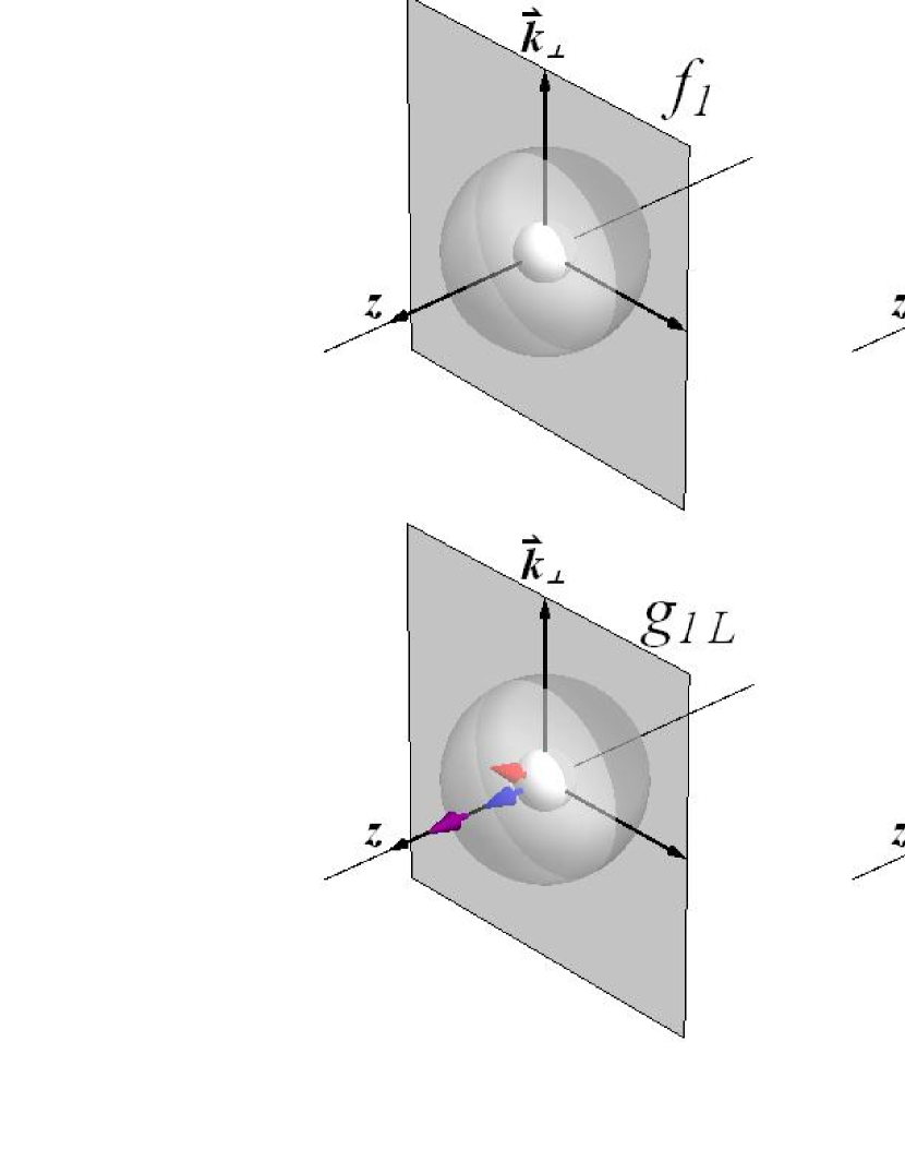
Figure 1: Connection between the TMDs and the amplitudes in the net-polarization basis. The $z$-axis corresponds to the light-cone direction. The $y$-axis in the transverse plane has been chosen parallel to the active quark transverse momentum $\boldsymbol{k}_{\perp}$. The arrows attached to the inner and outer spheres represent the net polarizations of the active quark and target, respectively, and absence of arrows represents the unpolarized case. Since we work in a frame where the target has no transverse momentum, there is no difference between target light-cone and canonical polarizations (purple outer arrows). TMDs in the light-cone basis are related to matrix elements where the quark net polarization is along the axes (blue inner arrows), while in the canonical-spin basis the component of quark net polarization in the $(y,z)$-plane is tilted with respect to the axes (red inner arrows), see text.

Playing a little bit with Eqs. (27) and (28), we find

$$\begin{pmatrix}\tfrac{k_{\perp}}{M}\left(g^{q}_{1T}+h_{1L}^{\perp q}\right)\\ g^{q}_{1L}-h_{1T}^{+q}\end{pmatrix}=\begin{pmatrix}\cos\theta&-\sin\theta\\ \sin\theta&\cos\theta\end{pmatrix}\begin{pmatrix}\tfrac{k_{\perp}}{M}\left(\mathfrak{g}^{q}_{1T}+\mathfrak{h}_{1L}^{\perp q}\right)\\ \mathfrak{g}^{q}_{1L}-\mathfrak{h}_{1T}^{+q}\end{pmatrix},$$ (32)

and three expressions invariant under the rotation (24)

$$\left(\tfrac{k_{\perp}}{M}\,g^{q}_{1T}\right)^{2}+\left(h_{1T}^{+q}\right)^{2} =\left(\tfrac{k_{\perp}}{M}\,\mathfrak{g}_{1T}^{q}\right)^{2}+\left(\mathfrak{h}_{1T}^{+q}\right)^{2},$$ (33)

$$\left(g^{q}_{1L}\right)^{2}+\left(\tfrac{k_{\perp}}{M}\,h_{1L}^{\perp q}\right)^{2} =\left(\mathfrak{g}_{1L}^{q}\right)^{2}+\left(\tfrac{k_{\perp}}{M}\,\mathfrak{h}_{1L}^{\perp q}\right)^{2},$$ (34)

$$g^{q}_{1L}\,g^{q}_{1T}+h_{1L}^{\perp q}\,h_{1T}^{+q} =\mathfrak{g}_{1L}^{q}\,\mathfrak{g}_{1T}^{q}+\mathfrak{h}_{1L}^{\perp q}\,\mathfrak{h}_{1T}^{+q}.$$ (35)

These three invariant expressions have a simple geometric interpretation. The three-component vector $\sum_{i}S^{i}\Phi_{q}^{ij}\equiv\pi^{qj}_{\boldsymbol{S}}$ represents the net light-cone polarization of a quark with three-momentum $(xP^{+},\boldsymbol{k}_{\perp})$ and flavor $q$ in a target with net polarization in the $\boldsymbol{S}$-direction. From Eq. (24), we see that the vector $\boldsymbol{\pi}^{q}_{C\boldsymbol{S}}$ representing the net canonical polarization of the quark is obtained by a rotation of $\boldsymbol{\pi}^{q}_{\boldsymbol{S}}$

$$\pi^{qj}_{C\boldsymbol{S}}=\sum_{k}\pi^{qk}_{\boldsymbol{S}}\,O^{kj}.$$ (36)

It follows automatically that $\boldsymbol{\pi}^{q}_{\boldsymbol{S}}\cdot\boldsymbol{\pi}^{q}_{\boldsymbol{S}^{\prime}}$ is invariant under the rotation (24)

$$\boldsymbol{\pi}^{q}_{\boldsymbol{S}}\cdot\boldsymbol{\pi}^{q}_{\boldsymbol{S}^{\prime}}=\boldsymbol{\pi}^{q}_{C\boldsymbol{S}}\cdot\boldsymbol{\pi}^{q}_{C\boldsymbol{S}^{\prime}}.$$ (37)

Expressions (33) and (34) are obtained from (37) for the cases $\boldsymbol{S}=\boldsymbol{S}^{\prime}=\boldsymbol{e}_{\perp}$ and $\boldsymbol{S}=\boldsymbol{S}^{\prime}=\boldsymbol{e}_{z}$, respectively. They just express the fact that the magnitude of quark net polarization is the same in the light-cone helicity and canonical-spin bases. Expression (35) is obtained for the case $\boldsymbol{S}=\boldsymbol{e}_{\perp}$ and $\boldsymbol{S}^{\prime}=\boldsymbol{e}_{z}$. All the remaining cases do not lead to new independent expressions.

IV.3 Spherical Symmetry

We are now ready to discuss the implications of spherical symmetry in the canonical-spin basis. Spherical symmetry means that the canonical tensor correlator has to be invariant $O_{R}^{T}\Phi_{Cq}O_{R}=\Phi_{Cq}$ under any spatial rotation $O_{R}=\left(\begin{smallmatrix}1&0\\ 0&R\end{smallmatrix}\right)$ with $R$ the ordinary $3\times 3$ rotation matrix. It is equivalent to the statement that the tensor correlator has to commute with all the elements of the rotation group $\Phi_{Cq}O_{R}=O_{R}\Phi_{Cq}$. As a result of Schur’s lemma, the canonical tensor correlator must have the following structure

$$\Phi^{\mu\nu}_{Cq}=\begin{pmatrix}A^{q}&0&0&0\\ 0&B^{q}&0&0\\ 0&0&B^{q}&0\\ 0&0&0&B^{q}\end{pmatrix}.$$ (38)

Comparing this with Eqs. (26) or (31), we conclude that spherical symmetry implies

$$f^{q}_{1}=A^{q},$$ (39)

$$\mathfrak{g}_{1L}^{q}=\mathfrak{h}_{1T}^{+q}=h_{1T}^{-q}=B^{q},$$ (40)

$$\mathfrak{g}_{1T}^{q}=\mathfrak{h}_{1L}^{\perp q}=f_{1T}^{\perp q}=h_{1}^{\perp q}=0.$$ (41)

Clearly, only the monopole structures in the canonical-spin basis are allowed to survive. In particular, the Sivers and Boer-Mulders functions $f_{1T}^{\perp q}$ and $h_{1}^{\perp q}$ have to vanish identically. However, as one can see from Figs. 2 and 3, the monopole structures in the canonical-spin basis generate higher multipole structures in the light-cone helicity basis. It follows that spherical symmetry imposes some relations among the multipole structures in the light-cone helicity basis, and therefore among the TMDs.

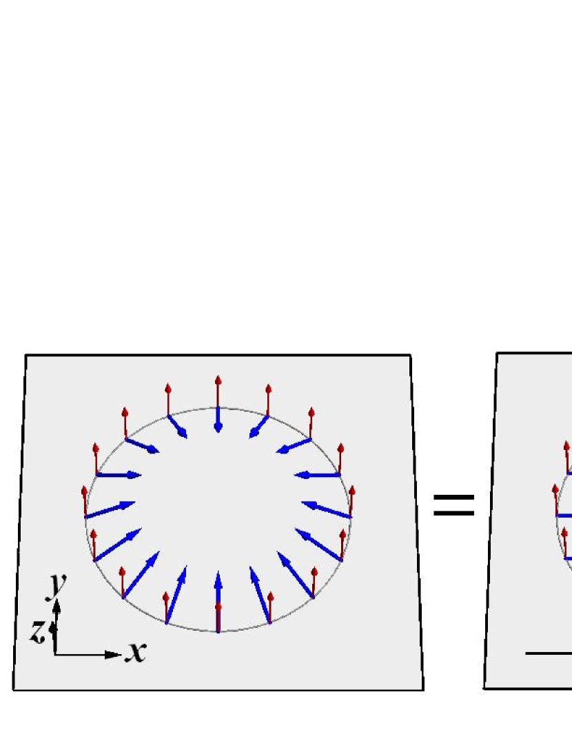
Figure 2: Net light-cone polarization (thick blue arrows) associated to a quark with net longitudinal canonical polarization (thin red arrows), and its vector decomposition along the three axes, for fixed $x$ and $k_{\perp}$ but arbitrary direction $\hat{k}_{\perp}$. The $x$- and $y$-components are pure dipoles, while the $z$-component is a pure monopole.

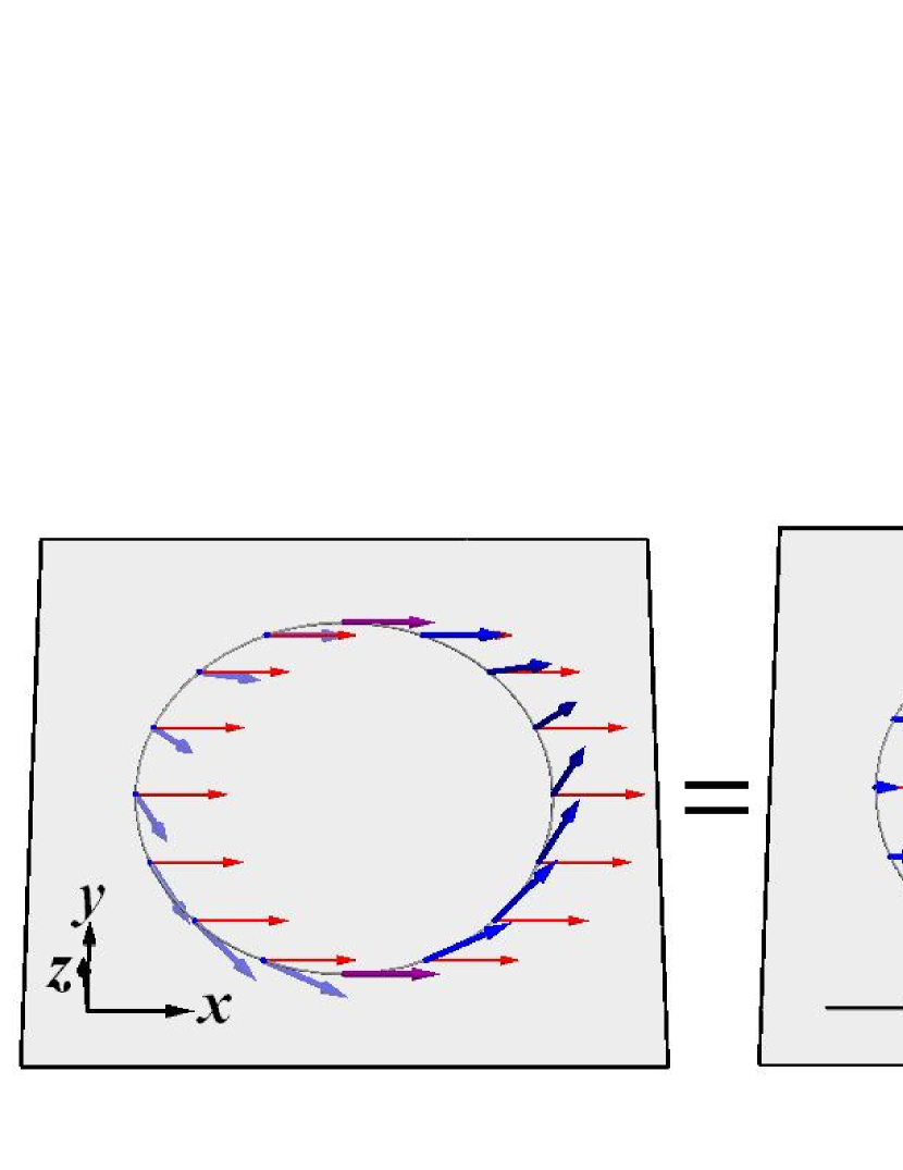
Figure 3: In the first line is shown the net light-cone polarization (thick blue arrows) associated to a quark with net canonical polarization in the $x$-direction (thin red arrows), and its vector decomposition along the three axes, for fixed $x$ and $k_{\perp}$ but arbitrary direction $\hat{k}_{\perp}$. The $y$-component is a pure quadrupole, and the $z$-component is a pure dipole. The $x$-component is the sum of a monopole and a quadrupole, as illustrated in the second line.

Inserting the constraints (40) and (41) into Eq. (32), we automatically obtain the linear relations (19) and (20)

$$\begin{pmatrix}\tfrac{k_{\perp}}{M}\left(g^{q}_{1T}+h_{1L}^{\perp q}\right)\\ g^{q}_{1L}-h_{1T}^{+q}\end{pmatrix}=\begin{pmatrix}0\\ 0\end{pmatrix}.$$ (42)

Using now the constraints from spherical symmetry in Eq. (33), we obtain the quadratic relation (21)

$$0=\left(\tfrac{k_{\perp}}{M}\,g^{q}_{1T}\right)^{2}+\left(h_{1T}^{+q}\right)^{2}-\left(h_{1T}^{-q}\right)^{2}=\tfrac{\boldsymbol{k}_{\perp}^{2}}{M^{2}}\left[\left(g^{q}_{1T}\right)^{2}+2h^{q}_{1}\,h_{1T}^{\perp q}\right].$$ (43)

The linear relations (19) and (20) being satisfied, the Eqs. (34) and (35) do not lead to independent quadratic relations.

We have seen that spherical symmetry is a sufficient condition to obtain all three flavor-independent relations. At the same time, it tells us that the Sivers and Boer-Mulders distributions have to vanish identically. Restricting ourselves to axial symmetries, we find that some of the relations can already be obtained. For example, axial symmetry about $\boldsymbol{e}_{z}$ alone implies $f_{1T}^{\perp}=h_{1}^{\perp}=0$, the quadratic relation (21) and

$$g^{q}_{1L}\,g^{q}_{1T}+h_{1L}^{\perp q}\,h_{1T}^{+q}=0.$$ (44)

Axial symmetry about $\hat{k}_{\perp}\times\boldsymbol{e}_{z}$ implies the two linear relations (19) and (20). The relation (44) is naturally also satisfied but is not independent.

V Wave-Function Approach

Many quark models are based on a wave-function approach. We therefore translate here the derivation of the previous section in the language of 3Q wave functions. The advantage is that we can then also discuss the additional $SU(6)$ spin-flavor symmetry needed for the flavor-dependent relation (22). For convenience, we omit all the color indices in the following expressions.

V.1 Overlap Representation of the TMDs on the Light Cone

Restricting ourselves to the 3Q Fock sector, the target state with definite four-momentum $P=[P^{+},\tfrac{M^{2}}{2P^{+}},\boldsymbol{0}_{\perp}]$ and light-cone helicity $\Lambda$ can be written as follows

$$|P,\Lambda\rangle=\sum_{\lambda_{1}\lambda_{2}\lambda_{3}}\sum_{q_{1}q_{2}q_{3}}\int[\mathrm{d}x]_{3}\,[\mathrm{d}^{2}k_{\perp}]_{3}\,\psi^{\Lambda;q_{1}q_{2}q_{3}}_{\lambda_{1}\lambda_{2}\lambda_{3}}(\tilde{k}_{1},\tilde{k}_{2},\tilde{k}_{3})\,|\{\lambda_{i},q_{i},\tilde{k}_{i}\}\rangle,$$ (45)

where $\psi^{\Lambda;q_{1}q_{2}q_{3}}_{\lambda_{1}\lambda_{2}\lambda_{3}}(\tilde{k}_{1},\tilde{k}_{2},\tilde{k}_{3})$ is the three-quark light-cone wave function (3Q LCWF) with $\lambda_{i}$, $q_{i}$ and $\tilde{k}_{i}$ referring to the light-cone helicity, flavor and light-cone momentum of quark $i$, respectively. The total orbital angular momentum of a given component $\psi^{\Lambda}_{\lambda_{1}\lambda_{2}\lambda_{3}}$ is given by the expression $\ell_{z}=\Lambda-\lambda_{1}-\lambda_{2}-\lambda_{3}$ with $\Lambda,\lambda_{i}=\pm\tfrac{1}{2}$. The integration measures in Eq. (45) are defined as

$$\begin{split}[\mathrm{d}x]_{3}&\equiv\left[\prod_{i=1}^{3}\mathrm{d}x_{i}\right]\delta\!\!\left(1-\sum_{i=1}^{3}x_{i}\right),\\ [\mathrm{d}^{2}k_{\perp}]_{3}&\equiv\left[\prod_{i=1}^{3}\frac{\mathrm{d}^{2}k_{i\perp}}{2(2\pi)^{3}}\right]2(2\pi)^{3}\,\delta^{(2)}\!\!\left(\sum_{i=1}^{3}\boldsymbol{k}_{i\perp}\right).\end{split}$$ (46)

Choosing to label the active quark with $i=1$, the TMDs can be obtained by the following overlaps of 3Q LCWFs

$$f^{q}_{1} =\int\mathrm{d}[23]\sum_{\lambda_{2}\lambda_{3}}\sum_{q_{2}q_{3}}\left[|\psi^{+;qq_{2}q_{3}}_{+\lambda_{2}\lambda_{3}}|^{2}+|\psi^{+;qq_{2}q_{3}}_{-\lambda_{2}\lambda_{3}}|^{2}\right],$$ (47a)

$$g^{q}_{1L} =\int\mathrm{d}[23]\sum_{\lambda_{2}\lambda_{3}}\sum_{q_{2}q_{3}}\left[|\psi^{+;qq_{2}q_{3}}_{+\lambda_{2}\lambda_{3}}|^{2}-|\psi^{+;qq_{2}q_{3}}_{-\lambda_{2}\lambda_{3}}|^{2}\right],$$ (47b)

$$h^{q}_{1} =\int\mathrm{d}[23]\sum_{\lambda_{2}\lambda_{3}}\sum_{q_{2}q_{3}}\left(\psi^{+;qq_{2}q_{3}}_{+\lambda_{2}\lambda_{3}}\right)^{*}\psi^{-;qq_{2}q_{3}}_{-\lambda_{2}\lambda_{3}},$$ (47c)

$$\tfrac{k_{\perp}}{M}\,f^{\perp q}_{1T} =\int\mathrm{d}[23]\sum_{\lambda_{2}\lambda_{3}}\sum_{q_{2}q_{3}}2\,\Im m\left[\hat{k}_{R}\left(\psi^{+;qq_{2}q_{3}}_{+\lambda_{2}\lambda_{3}}\right)^{*}\psi^{-;qq_{2}q_{3}}_{+\lambda_{2}\lambda_{3}}\right],$$ (47d)

$$\tfrac{k_{\perp}}{M}\,g^{q}_{1T} =\int\mathrm{d}[23]\sum_{\lambda_{2}\lambda_{3}}\sum_{q_{2}q_{3}}2\,\Re e\left[\hat{k}_{R}\left(\psi^{+;qq_{2}q_{3}}_{+\lambda_{2}\lambda_{3}}\right)^{*}\psi^{-;qq_{2}q_{3}}_{+\lambda_{2}\lambda_{3}}\right],$$ (47e)

$$\tfrac{k_{\perp}}{M}\,h^{\perp q}_{1} =\int\mathrm{d}[23]\sum_{\lambda_{2}\lambda_{3}}\sum_{q_{2}q_{3}}2\,\Im m\left[\hat{k}_{R}\left(\psi^{+;qq_{2}q_{3}}_{-\lambda_{2}\lambda_{3}}\right)^{*}\psi^{+;qq_{2}q_{3}}_{+\lambda_{2}\lambda_{3}}\right],$$ (47f)

$$\tfrac{k_{\perp}}{M}\,h^{\perp q}_{1L} =\int\mathrm{d}[23]\sum_{\lambda_{2}\lambda_{3}}\sum_{q_{2}q_{3}}2\,\Re e\left[\hat{k}_{R}\left(\psi^{+;qq_{2}q_{3}}_{-\lambda_{2}\lambda_{3}}\right)^{*}\psi^{+;qq_{2}q_{3}}_{+\lambda_{2}\lambda_{3}}\right],$$ (47g)

$$\tfrac{\boldsymbol{k}_{\perp}^{2}}{2M^{2}}\,h^{\perp q}_{1T} =\int\mathrm{d}[23]\sum_{\lambda_{2}\lambda_{3}}\sum_{q_{2}q_{3}}\hat{k}^{2}_{R}\left(\psi^{+;qq_{2}q_{3}}_{-\lambda_{2}\lambda_{3}}\right)^{*}\psi^{-;qq_{2}q_{3}}_{+\lambda_{2}\lambda_{3}},$$ (47h)

where we used the notation

$$\mathrm{d}[23]=[\mathrm{d}x]_{3}\,[\mathrm{d}^{2}k_{\perp}]_{3}\,3\,\delta(x-x_{1})\,\delta^{(2)}(\boldsymbol{k}_{\perp}-\boldsymbol{k}_{1\perp}).$$ (48)

Clearly, the TMDs associated to the monopole structures ($f^{q}_{1},g^{q}_{1L},h^{q}_{1}$) are represented by overlaps with no global change of orbital angular momentum $\Delta\ell_{z}=0$, the ones associated to the dipole structures ($f_{1T}^{\perp q},g^{q}_{1T},h_{1}^{\perp q},h_{1L}^{\perp q}$) involve a change by one unit of orbital angular momentum $|\Delta\ell_{z}|=1$ and the one associated to the quadrupole structure ($h_{1T}^{\perp q}$) involves a change by two units of orbital angular momentum $|\Delta\ell_{z}|=2$.

V.2 Overlap Representation of the TMDs in the Canonical-Spin Basis

Most of the quark models being originally formulated in the instant form, it is more natural to work in the canonical-spin basis instead of the light-cone helicity basis. Since we considered a frame where the target has no transverse momentum, there is no difference between target light-cone and canonical polarizations. Assuming that the quark light-cone helicity and canonical spin are connected by the rotation in Eq. (23), the components of the LCWF in the canonical-spin basis $\psi^{\Lambda}_{\sigma_{1}\sigma_{2}\sigma_{3}}$ (with $\sigma_{i}=\uparrow,\downarrow$) and in the light-cone helicity basis $\psi^{\Lambda}_{\lambda_{1}\lambda_{2}\lambda_{3}}$ (with $\lambda_{i}=\pm$) are related as follows

$$\psi^{\Lambda}_{\lambda_{1}\lambda_{2}\lambda_{3}}=\sum_{\sigma_{1}\sigma_{2}\sigma_{3}}\psi^{\Lambda}_{\sigma_{1}\sigma_{2}\sigma_{3}}\,D^{(1/2)*}_{\sigma_{1}\lambda_{1}}\,D^{(1/2)*}_{\sigma_{2}\lambda_{2}}\,D^{(1/2)*}_{\sigma_{3}\lambda_{3}}.$$ (49)

The correspondence between the components in the two polarization bases is given in a more explicit form in App. B. Using $D^{(1/2){\dagger}}D^{(1/2)}=\mathds{1}$, we find the explicit overlap representations in canonical-spin basis

$$f^{q}_{1} =\int\mathrm{d}[23]\sum_{\sigma_{2}\sigma_{3}}\sum_{q_{2}q_{3}}\left[|\psi^{\uparrow;qq_{2}q_{3}}_{\uparrow\sigma_{2}\sigma_{3}}|^{2}+|\psi^{\uparrow;qq_{2}q_{3}}_{\downarrow\sigma_{2}\sigma_{3}}|^{2}\right],$$ (50a)

$$\mathfrak{g}^{q}_{1L} =\int\mathrm{d}[23]\sum_{\sigma_{2}\sigma_{3}}\sum_{q_{2}q_{3}}\left[|\psi^{\uparrow;qq_{2}q_{3}}_{\uparrow\sigma_{2}\sigma_{3}}|^{2}-|\psi^{\uparrow;qq_{2}q_{3}}_{\downarrow\sigma_{2}\sigma_{3}}|^{2}\right],$$ (50b)

$$\mathfrak{h}_{1}^{q} =\int\mathrm{d}[23]\sum_{\sigma_{2}\sigma_{3}}\sum_{q_{2}q_{3}}\left(\psi^{\uparrow;qq_{2}q_{3}}_{\uparrow\sigma_{2}\sigma_{3}}\right)^{*}\psi^{\downarrow;qq_{2}q_{3}}_{\downarrow\sigma_{2}\sigma_{3}},$$ (50c)

$$\tfrac{k_{\perp}}{M}\,f^{\perp q}_{1T} =\int\mathrm{d}[23]\sum_{\sigma_{2}\sigma_{3}}\sum_{q_{2}q_{3}}2\,\Im m\left[\hat{k}_{R}\left(\psi^{\uparrow;qq_{2}q_{3}}_{\uparrow\sigma_{2}\sigma_{3}}\right)^{*}\psi^{\downarrow;qq_{2}q_{3}}_{\uparrow\sigma_{2}\sigma_{3}}\right],$$ (50d)

$$\tfrac{k_{\perp}}{M}\,\mathfrak{g}^{q}_{1T} =\int\mathrm{d}[23]\sum_{\sigma_{2}\sigma_{3}}\sum_{q_{2}q_{3}}2\,\Re e\left[\hat{k}_{R}\left(\psi^{\uparrow;qq_{2}q_{3}}_{\uparrow\sigma_{2}\sigma_{3}}\right)^{*}\psi^{\downarrow;qq_{2}q_{3}}_{\uparrow\sigma_{2}\sigma_{3}}\right],$$ (50e)

$$\tfrac{k_{\perp}}{M}\,h^{\perp}_{1} =\int\mathrm{d}[23]\sum_{\sigma_{2}\sigma_{3}}\sum_{q_{2}q_{3}}2\,\Im m\left[\hat{k}_{R}\left(\psi^{\uparrow;qq_{2}q_{3}}_{\downarrow\sigma_{2}\sigma_{3}}\right)^{*}\psi^{\uparrow;qq_{2}q_{3}}_{\uparrow\sigma_{2}\sigma_{3}}\right],$$ (50f)

$$\tfrac{k_{\perp}}{M}\,\mathfrak{h}^{\perp q}_{1L} =\int\mathrm{d}[23]\sum_{\sigma_{2}\sigma_{3}}\sum_{q_{2}q_{3}}2\,\Re e\left[\hat{k}_{R}\left(\psi^{\uparrow;qq_{2}q_{3}}_{\downarrow\sigma_{2}\sigma_{3}}\right)^{*}\psi^{\uparrow;qq_{2}q_{3}}_{\uparrow\sigma_{2}\sigma_{3}}\right],$$ (50g)

$$\tfrac{\boldsymbol{k}_{\perp}^{2}}{2M^{2}}\,\mathfrak{h}^{\perp q}_{1T} =\int\mathrm{d}[23]\sum_{\sigma_{2}\sigma_{3}}\sum_{q_{2}q_{3}}\hat{k}^{2}_{R}\left(\psi^{\uparrow;qq_{2}q_{3}}_{\downarrow\sigma_{2}\sigma_{3}}\right)^{*}\psi^{\downarrow;qq_{2}q_{3}}_{\uparrow\sigma_{2}\sigma_{3}},$$ (50h)

with $\mathfrak{h}_{1T}^{+q}=\mathfrak{h}^{q}_{1}+\tfrac{\boldsymbol{k}_{\perp}^{2}}{2M^{2}}\,\mathfrak{h}_{1T}^{\perp q}$ and $h_{1T}^{-q}=\mathfrak{h}^{q}_{1}-\tfrac{\boldsymbol{k}_{\perp}^{2}}{2M^{2}}\,\mathfrak{h}_{1T}^{\perp q}$. The functions $\mathfrak{g}^{q}_{1L},\mathfrak{g}^{q}_{1T},\mathfrak{h}^{\perp q}_{1L},\mathfrak{h}^{+q}_{1T}$ are again related to the TMDs $g^{q}_{1L},g^{q}_{1T},h^{\perp q}_{1L},h^{+q}_{1T}$ according to Eqs. (27) and (28).

V.3 Spherical Symmetry

We now discuss how spherical symmetry restricts the form of the wave function in the canonical-spin basis. Spherical symmetry requires the wave function to be invariant under any rotation, i.e.

$$\sum_{\Lambda^{\prime}\sigma^{\prime}_{1}\sigma^{\prime}_{2}\sigma^{\prime}_{3}}\left[u(\theta,\phi)\right]_{\sigma_{1}\sigma^{\prime}_{1}}\left[u(\theta,\phi)\right]_{\sigma_{2}\sigma^{\prime}_{2}}\left[u(\theta,\phi)\right]_{\sigma_{3}\sigma^{\prime}_{3}}\left[u(\theta,\phi)\right]^{*}_{\Lambda\Lambda^{\prime}}\psi^{\Lambda^{\prime}}_{\sigma^{\prime}_{1}\sigma^{\prime}_{2}\sigma^{\prime}_{3}}=\psi^{\Lambda}_{\sigma_{1}\sigma_{2}\sigma_{3}},$$ (51)

with the $SU(2)$ rotation matrix $u(\theta,\phi)$ given by Eq. (12). In particular, invariance under a $(\pi,0)$-rotation leads to

$$\psi^{-\Lambda}_{-\sigma_{1}-\sigma_{2}-\sigma_{3}}=(-1)^{\Lambda+\sigma_{1}+\sigma_{2}+\sigma_{3}}\,\psi^{\Lambda}_{\sigma_{1}\sigma_{2}\sigma_{3}},$$ (52)

while invariance under $(0,\phi)$-rotations implies that all components with $\ell_{z}\neq 0$ have to vanish

$$\psi^{\uparrow}_{\uparrow\uparrow\uparrow}=\psi^{\uparrow}_{\downarrow\downarrow\uparrow}=\psi^{\uparrow}_{\downarrow\uparrow\downarrow}=\psi^{\uparrow}_{\uparrow\downarrow\downarrow}=\psi^{\uparrow}_{\downarrow\downarrow\downarrow}=0.$$ (53)

Taking into account the constraints (52) and (53) in an arbitrary $(\theta,\phi)$-rotation, one finally gets

$$\psi^{\uparrow}_{\uparrow\uparrow\downarrow}+\psi^{\uparrow}_{\uparrow\downarrow\uparrow}+\psi^{\uparrow}_{\downarrow\uparrow\uparrow}=0.$$ (54)

Again, spherical symmetry implies that the TMDs are either identically zero or proportional to the unpolarized and polarized amplitudes $A^{q}$ and $B^{q}$,

$$f^{q}_{1} =A^{q},$$ (55a)

$$g^{q}_{1L} =\cos\theta\,B^{q},$$ (55b)

$$h^{q}_{1} =\frac{\cos\theta+1}{2}\,B^{q},$$ (55c)

$$\tfrac{k_{\perp}}{M}\,f^{\perp q}_{1T} =0,$$ (55d)

$$\tfrac{k_{\perp}}{M}\,g^{q}_{1T} =\sin\theta\,B^{q},$$ (55e)

$$\tfrac{k_{\perp}}{M}\,h^{\perp q}_{1} =0,$$ (55f)

$$\tfrac{k_{\perp}}{M}\,h^{\perp q}_{1L} =-\sin\theta\,B^{q},$$ (55g)

$$\tfrac{\boldsymbol{k}_{\perp}^{2}}{2M^{2}}\,h^{\perp q}_{1T} =\frac{\cos\theta-1}{2}\,B^{q},$$ (55h)

with $A^{q}$ and $B^{q}$ given by the following overlaps

$$A^{q} =\int\mathrm{d}[23]\sum_{q_{2}q_{3}}\left[|\psi^{\uparrow;qq_{2}q_{3}}_{\uparrow\uparrow\downarrow}|^{2}+|\psi^{\uparrow;qq_{2}q_{3}}_{\uparrow\downarrow\uparrow}|^{2}+|\psi^{\uparrow;qq_{2}q_{3}}_{\downarrow\uparrow\uparrow}|^{2}\right],$$ (56)

$$B^{q} =\int\mathrm{d}[23]\sum_{q_{2}q_{3}}\left[|\psi^{\uparrow;qq_{2}q_{3}}_{\uparrow\uparrow\downarrow}|^{2}+|\psi^{\uparrow;qq_{2}q_{3}}_{\uparrow\downarrow\uparrow}|^{2}-|\psi^{\uparrow;qq_{2}q_{3}}_{\downarrow\uparrow\uparrow}|^{2}\right]$$

$$=\int\mathrm{d}[23]\sum_{q_{2}q_{3}}\left[\left(\psi^{\uparrow;qq_{2}q_{3}}_{\uparrow\uparrow\downarrow}\right)^{*}\psi^{\downarrow;qq_{2}q_{3}}_{\downarrow\uparrow\downarrow}+\left(\psi^{\uparrow;qq_{2}q_{3}}_{\uparrow\downarrow\uparrow}\right)^{*}\psi^{\downarrow;qq_{2}q_{3}}_{\downarrow\downarrow\uparrow}\right].$$ (57)

The TMD relations (19)-(21) then follow trivially.

V.4 $SU(6)$ Spin-Flavor Symmetry

Many quark models, in addition of being spherically symmetric, assume also the $SU(6)$ spin-flavor symmetry. This symmetry restricts further the components of the wave function in the canonical-spin basis in the following way

$$\psi^{\uparrow;q_{1}q_{2}q_{3}}_{\sigma_{1}\sigma_{2}\sigma_{3}}$$

(58)

with $\phi=\phi(\{\tilde{k}_{i}\})$ some symmetric momentum wave function. This implies that the unpolarized and polarized amplitudes $A^{q}$ and $B^{q}$ are simply proportional

$$A^{u}=2A^{d}=\tfrac{3}{2}\,B^{u}=-6\,B^{d}=12\int\mathrm{d}[23]|\phi|^{2},$$ (59)

and so the flavor-dependent relation (22) follows trivially with $\mathcal{D}^{q}=B^{q}/A^{q}$.

VI Quark Models

In this section we review different quark models which have been used for the calculation of TMDs. In particular, we summarize the main ingredients of the models and discuss whether they satisfy the conditions of Sec. III. In order to facilitate the discussion, we sort the quark models in classes defined as follows:

• The light-cone constituent quark model (LCCQM) of Ref. Pasquini:2008ax and the light-cone quark-diquark model (LCQDM) of Refs. She:2009jq ; Zhu:2011zza constitute the class of light-cone models;

• The covariant parton model of Ref. Efremov:2009ze constitutes its own class;

• The bag model of Refs. Avakian:2010br ; Avakian:2008dz and the light-cone version of the chiral quark-soliton model ($\chi$QSM) of Refs. Lorce:2011dv ; Lorce:2006nq ; Lorce:2007as constitute the class of mean-field models;

• The quark-diquark models of Refs. Jakob:1997wg ; Goldstein:2002vv ; Gamberg:2003ey ; Gamberg:2007wm ; Bacchetta:2008af constitute the class of spectator models.

We do not discuss the quark-target model of Ref. Meissner:2007rx as it deals with gluons and therefore does already not satisfy the first condition of Sec. III.

VI.1 Light-Cone Models

The class of light-cone models is characterized by the fact that the target state is expanded in the basis of free parton (Fock) states. One usually truncates the expansion and considers only the state with the lowest number of partons. In the LCCQM, this lowest state consists of three valence quarks, while in the LCQDM it consists of a valence quark and a spectator diquark.

It is well known that light-cone helicity and canonical spin of free partons are simply related by the so-called Melosh rotation Melosh:1974cu . Its $j=1/2$ and $j=1$ representations Ahluwalia:1993xa are given by (see App. A for the definition of the spinors and polarization four-vectors)

$$D^{(1/2)*}_{\sigma\lambda}(\tilde{k}) =\frac{\overline{u}_{LC}(k,\lambda)u(k,\sigma)}{2m}$$

$$=\frac{1}{\sqrt{N}}\begin{pmatrix}\sqrt{2}\,k^{+}+m&-k_{R}\\ k_{L}&\sqrt{2}\,k^{+}+m\end{pmatrix},$$ (60)

$$D^{(1)*}_{\sigma\lambda}(\tilde{k}) =-\varepsilon^{*}_{LC}(k,\lambda)\cdot\varepsilon(k,\sigma)$$

$$=\frac{1}{N}\begin{pmatrix}\left(\sqrt{2}\,k^{+}+m\right)^{2}&-\sqrt{2}\left(\sqrt{2}\,k^{+}+m\right)k_{R}&k_{R}^{2}\\ \sqrt{2}\left(\sqrt{2}\,k^{+}+m\right)k_{L}&\left(\sqrt{2}\,k^{+}+m\right)^{2}-\boldsymbol{k}_{\perp}^{2}&-\sqrt{2}\left(\sqrt{2}\,k^{+}+m\right)k_{R}\\ k_{L}^{2}&\sqrt{2}\left(\sqrt{2}\,k^{+}+m\right)k_{L}&\left(\sqrt{2}\,k^{+}+m\right)^{2}\end{pmatrix},$$ (61)

where $m$ is the parton mass and $N=(\sqrt{2}\,k^{+}+m)^{2}+\boldsymbol{k}_{\perp}^{2}$. The LCWF in the canonical-spin basis being identified in these models with the instant-form wave function, it follows that $\sqrt{2}\,k^{+}=x\mathcal{M}_{0}$ with $\mathcal{M}_{0}=\sum_{i}\omega_{i}$ the mass of the free parton state and $\omega_{i}$ the free energy of parton $i$. Comparing now Eqs. (60) and (61) with Eqs. (23) and (93), we obtain

$$\cos\tfrac{\theta}{2}=\frac{m+x\mathcal{M}_{0}}{\sqrt{N}}\qquad\text{and}\qquad\sin\tfrac{\theta}{2}=\frac{k_{\perp}}{\sqrt{N}}.$$ (62)

Finally, both the LCCQM and LCQDM consider wave functions with spherical symmetry and $SU(6)$ spin-flavor symmetry. In other words, all the conditions of Sec. III are satisfied in these models, and so are the TMD relations (19)-(22).

VI.2 Covariant Parton Model

The standard quark-parton model (QPM) refers to the infinite momentum frame (IMF), where the parton mass can be neglected. The covariant parton model is an alternative to the QPM that is not confined to a preferred reference frame. Following the standard assumptions of the QPM, the covariant parton model describes the target system as a gas of quasi-free partons, i.e. the partons bound inside the target behave at the interaction with the external probe (at sufficiently high $Q^{2}$) as free particles having four-momenta on the mass shell. However, since the covariant parton model does not refer specifically to the IMF, the parton mass $m$ is not neglected. One also assumes explicitly that the parton phase space is spherical.

The covariant parton model does not refer explicitly to quark canonical spin or light-cone helicity. Instead, it deals with the covariant quark polarization vector. Identifying in the Bjorken limit the Lorentz structures of the hadronic tensor with those of the TMD correlator, the authors of Ref. Efremov:2009ze found that the TMDs are given in the covariant parton model by

$$f^{q}_{1} =\tfrac{1}{2}\left[\left(m+xM\right)^{2}+\boldsymbol{k}^{2}_{\perp}\right]\int\{\mathrm{d}\tilde{k}^{1}\},$$ (63a)

$$g^{q}_{1L} =\tfrac{1}{2}\left[\left(m+xM\right)^{2}-\boldsymbol{k}^{2}_{\perp}\right]\int\{\mathrm{d}k^{1}\},$$ (63b)

$$\tfrac{k_{\perp}}{M}\,f^{\perp q}_{1T} =0,$$ (63c)

$$\tfrac{k_{\perp}}{M}\,g^{q}_{1T} =\left(m+xM\right)k_{\perp}\int\{\mathrm{d}k^{1}\},$$ (63d)

$$\tfrac{k_{\perp}}{M}\,h^{\perp q}_{1} =0,$$ (63e)

$$\tfrac{k_{\perp}}{M}\,h^{\perp q}_{1L} =-\left(m+xM\right)k_{\perp}\int\{\mathrm{d}k^{1}\},$$ (63f)

$$\tfrac{\boldsymbol{k}_{\perp}^{2}}{2M^{2}}\,h^{\perp q}_{1T} =-\tfrac{1}{2}\,\boldsymbol{k}_{\perp}^{2}\int\{\mathrm{d}k^{1}\},$$ (63g)

where $M$ is the target mass, $\{\mathrm{d}\tilde{k}^{1}\}$ and $\{\mathrm{d}k^{1}\}$ are the measures associated to the distributions of unpolarized and polarized quarks, respectively. Comparing with Eq. (55), we find that

$$\cos\tfrac{\theta}{2}=\frac{m+xM}{\sqrt{\left(m+xM\right)^{2}+\boldsymbol{k}_{\perp}^{2}}}\qquad\text{and}\qquad\sin\tfrac{\theta}{2}=\frac{k_{\perp}}{\sqrt{\left(m+xM\right)^{2}+\boldsymbol{k}_{\perp}^{2}}},$$ (64)

which is nothing else than the Melosh rotation. This is consistent with the fact that the active quark is quasi-free in this model. The difference with light-cone models is that the physical mass of the target $M$ is used in the Melosh rotation instead of the free invariant mass $\mathcal{M}_{0}$. The conditions 1-3 of Sec. III are therefore satisfied in the covariant parton model, and so are the TMD relations (19)-(21). Since this model does not use the language of wave functions, the implementation of $SU(6)$ spin-flavor symmetry is more delicate and one has to assume that the unpolarized and polarized distributions become simply proportional in order to recover the TMD relation (22).

VI.3 Mean-Field Models

In mean-field models, the target is considered as made of quarks bound by a classical mean field representing the non-perturbative (long-range) contribution of the gluon field. Accordingly, the positive-frequency part of the quark field appearing in the definition of the correlator (1) is expanded in the basis of the bound-state solutions $e^{-iE_{n}t}\,\varphi_{n}(k,\sigma)$ instead of the free Dirac light-cone spinors $e^{-ip\cdot x}\,u_{LC}(k,\lambda)$. Moreover, one truncates the expansion to the lowest mode $\varphi\equiv\varphi_{1}$ with energy $E_{\text{lev}}\equiv E_{1}$.

In these models, the bound-state solution $\varphi(k,\sigma)$ is called the quark wave function. This object is clearly different from the LCWF introduced in Sec. V. In particular, the former is a spinor while the latter is an ordinary scalar function. It is however possible to relate them. Since we consider twist-$2$ Dirac operators $\Gamma$, only the good components of the spinors are involved in the quark bilinear $\overline{\varphi}(k,\sigma^{\prime})\Gamma\varphi(k,\sigma)$. Using $u^{\dagger}_{G}(\lambda)=P_{+}u_{LC}(k,\lambda)/\sqrt{2^{1/2}k^{+}}$ (see App. A), we find that

$$\overline{\varphi}(k,\sigma^{\prime})\Gamma\varphi(k,\sigma) =\varphi^{\dagger}(k,\sigma^{\prime})P_{+}\gamma^{0}\Gamma P_{+}\varphi(k,\sigma)$$

$$=\sum_{\lambda\lambda^{\prime}}F^{*}_{\lambda^{\prime}\sigma^{\prime}}(k^{\prime})\,F_{\lambda\sigma}(k)\,\frac{\overline{u}_{LC}(k,\lambda^{\prime})\Gamma u_{LC}(k,\lambda)}{\sqrt{2}k^{+}},$$ (65)

where we have defined $F_{\lambda\sigma}(k)=u^{\dagger}_{G}(\lambda)\varphi(k,\sigma)$. In agreement with Petrov:2002jr ; Diakonov:2005ib where one boosts explicitly the system in the mean-field approximation to the IMF, $F_{\lambda\sigma}(k)$ can be interpreted as the quark LCWF with $k_{z}=xM-E_{\text{lev}}$. The mass $M$ is identified with the nucleon mass $M_{N}$ in the bag model and with the soliton mass $\mathcal{M}_{N}$ in the $\chi$QSM.

The mean field is assumed spherically symmetric in the target rest frame. It follows that the lowest quark-state solution in momentum space takes the form

$$\varphi(k,\sigma)=\begin{pmatrix}f(|\boldsymbol{k}|)\\ \tfrac{\boldsymbol{k}\cdot\boldsymbol{\sigma}}{|\boldsymbol{k}|}\,g(|\boldsymbol{k}|)\end{pmatrix}\chi_{\sigma},$$ (66)

with $\chi_{\sigma}$ the Pauli spinor. The functions $f$ and $g$ in Eq. (66) represent the $s$ ($\ell=0$) and $p$ ($\ell=1$) waves of the bound-state solution. On the other hand, the general 3Q LCWF for a spin-$1/2$ target involves usually $s$-, $p$- and $d$-waves. There is no contradiction between these two statements since $f$ and $g$ describe a single quark in the target and therefore do not represent partial waves of total angular momentum. Note also that in the language of 3Q LCWF, the $s$-, $p$- and $d$-waves refer to components with $\ell_{z}=0$, $\pm 1$ and $\pm 2$, respectively. This is an abuse of language as partial waves should refer to $\ell$ and not $\ell_{z}$.

The quark LCWF corresponding to (66) is then given by

$$F_{\lambda\sigma}(k)=\frac{1}{\sqrt{2}}\begin{pmatrix}f(|\boldsymbol{k}|)+\tfrac{k_{z}}{|\boldsymbol{k}|}\,g(|\boldsymbol{k}|)&-\tfrac{k_{R}}{|\boldsymbol{k}|}\,g(|\boldsymbol{k}|)\\ \tfrac{k_{L}}{|\boldsymbol{k}|}\,g(|\boldsymbol{k}|)&f(|\boldsymbol{k}|)+\tfrac{k_{z}}{|\boldsymbol{k}|}\,g(|\boldsymbol{k}|)\end{pmatrix}_{\sigma\lambda}.$$ (67)

It describes in particular how canonical spin $\sigma$ and light-cone helicity $\lambda$ are related. Comparing with Eq. (23), we find that

$$\cos\tfrac{\theta}{2}=\frac{f(|\boldsymbol{k}|)+\tfrac{k_{z}}{|\boldsymbol{k}|}\,g(|\boldsymbol{k}|)}{\sqrt{N}}\qquad\text{and}\qquad\sin\tfrac{\theta}{2}=\frac{\tfrac{k_{\perp}}{|\boldsymbol{k}|}\,g(|\boldsymbol{k}|)}{\sqrt{N}},$$ (68)

with $N=f^{2}(|\boldsymbol{k}|)+2\,\tfrac{k_{z}}{|\boldsymbol{k}|}\,f(|\boldsymbol{k}|)g(|\boldsymbol{k}|)+g^{2}(|\boldsymbol{k}|)$. The 3Q LCWF written as $\prod_{i=1}^{3}F_{\lambda_{i}\sigma_{i}}(k_{i})$ times the standard $SU(6)$ spin-flavor wave function with target polarization $\Lambda=\sum_{i}\sigma_{i}$, is then consistent with spherical symmetry in the canonical-spin basis. All the conditions of Section III being satisfied in mean-field models, the TMD relations (19)-(22) follow automatically.

VI.4 Spectator Models

The basic idea of spectator models is to evaluate the quark-quark correlator $\Phi$ of Eq. (1) by inserting a complete set of intermediate states and then truncating this set at tree level to a single on-shell spectator diquark state, i.e. a state with the quantum numbers of two quarks. The diquark can be either an isospin singlet with spin $0$ (scalar diquark) or an isospin triplet with spin $1$ (axial-vector diquark). The target is then seen as made of an off-shell quark and an on-shell diquark. Spectator models differ by their specific choice of target-quark-diquark vertices, polarization four-vectors associated with the axial-vector diquark, and form factors which take into account in an effective way the composite nature of the target and the spectator diquark.

As advocated in Ref. Brodsky:2000ii , the parton distributions can conveniently be computed using the language of LCWFs. The scalar quark-diquark LCWF is defined as

$$\psi^{\Lambda}_{\lambda}(\tilde{k})\propto\overline{u}_{LC}(k,\lambda)\mathcal{Y}_{s}u_{LC}(P,\Lambda)$$ (69)

with target momentum $P=\left[P^{+},\tfrac{M^{2}}{2P^{+}},\boldsymbol{0}_{\perp}\right]$. We do not need to specify all the factors in the definition as we are only interested in the structure of the wave function in the light-cone helicity basis. The scalar vertex is of the Yukawa type $\mathcal{Y}_{s}=g_{s}(k^{2})\,\mathds{1}$ with $g_{s}(k^{2})$ some form factor. Writing down explicitly the components, one finds

$$\psi^{\Lambda}_{\lambda}(\tilde{k})\propto\frac{g_{s}(k^{2})}{\sqrt{x}}\begin{pmatrix}m+xM&-k_{R}\\ k_{L}&m+xM\end{pmatrix}_{\Lambda\lambda}.$$ (70)

Note the striking resemblance with the Melosh rotation matrix of Eq. (60). One can similarly define a rest-frame scalar quark-diquark wave function as

$$\Psi^{\Lambda}_{\sigma}\propto\overline{u}(k,\sigma)\mathcal{Y}_{s}u(P_{\text{rest}},\Lambda)=g_{s}(k^{2})\sqrt{2M(E+m)}\,\delta_{\Lambda\sigma}$$ (71)

with target momentum $P_{\text{rest}}=\left(M,\boldsymbol{0}\right)$. This wave function is obviously spherically symmetric . Furthermore, Eq. (70) suggests that the quark light-cone helicity and canonical spin are simply related by a Melosh rotation, as if the quark was free Ellis:2008in . In other words, the conditions 1-3 of Section III are satisfied in scalar diquark models with Yukawa-like vertex, and so are the TMD relations (19)-(21).

The axial-vector quark-diquark LCWF is defined as

$$\psi^{\Lambda}_{\lambda\lambda_{D}}(\tilde{k})\propto\overline{u}_{LC}(k,\lambda)\varepsilon^{*}_{LC\mu}(K,\lambda_{D})\mathcal{Y}^{\mu}_{a}u_{LC}(P,\Lambda).$$ (72)

The spectator model of Jakob et al. Jakob:1997wg assumes the following structure for the axial-vector vertex $\mathcal{Y}^{\mu}_{a}=\frac{g_{a}(k^{2})}{\sqrt{3}}\,\gamma_{5}\left(\gamma^{\mu}+\tfrac{P^{\mu}}{M}\right)$ and the following momentum argument for the polarization four-vector $K=P$. The motivation for such a choice is to ensure that, in the target rest frame, the diquark spin-$1$ states are purely spatial. Indeed, the rest-frame axial-vector quark-diquark wave function reads in this model

$$\Psi^{\Lambda}_{\sigma\sigma_{D}}\propto\overline{u}(k,\sigma)\varepsilon^{*}_{\mu}(K,\sigma_{D})\mathcal{Y}^{\mu}_{a}u(P_{\text{rest}},\Lambda)=\frac{g_{a}(k^{2})}{\sqrt{3}}\,\sqrt{2M(E+m)}\left(\boldsymbol{\epsilon}_{\sigma_{D}}\cdot\boldsymbol{\sigma}\right)_{\sigma\Lambda}.$$ (73)

It satisfies the constraints (97) and is therefore spherically symmetric. Writing down explicitly the components of the corresponding LCWF, one finds

$$\begin{gathered}\psi^{+}_{+0}\propto\frac{g_{a}(k^{2})}{\sqrt{3x}}\left(m+xM\right),\qquad\psi^{+}_{-0}\propto-\frac{g_{a}(k^{2})}{\sqrt{3x}}\,k_{R},\\ \psi^{+}_{-+}=-\sqrt{2}\,\psi^{+}_{+0},\qquad\psi^{-}_{--}=\sqrt{2}\,\psi^{+}_{-0},\qquad\psi^{+}_{+-}=\psi^{+}_{--}=0,\end{gathered}$$ (74)

the other components being given by $\psi^{-\Lambda}_{-\lambda-\lambda_{D}}=(-1)^{\Lambda+\lambda+\lambda_{D}}\left(\psi^{\Lambda}_{\lambda\lambda_{D}}\right)^{*}$, with $\Lambda,\lambda=\pm\tfrac{1}{2}$ and $\lambda_{D}=+1,0,-1$. Again, one recognizes the characteristic factors of the Melosh rotation Ellis:2008in . Comparing the structure of the components of the LCWF in Eq. (74) with the structure of the components of the LCWF given in Table 3 after applying the constraints of spherical symmetry in the canonical-spin basis (97), one concludes that only the quark polarization is rotated. This is in agreement with the fact that the momentum argument of the polarization four-vector $\varepsilon_{\mu}$ does not have any transverse momentum, and so there is no rotation of the diquark polarization. All the conditions 1-3 of Section III being satisfied in the axial-vector diquark model of Ref. Jakob:1997wg , the TMD relations (19)-(21) follow automatically. The flavor-dependent relation (22) can be obtained by further imposing $SU(6)$ spin-flavor symmetry to the wave function.

On the contrary, some versions of the spectator model presented by Bacchetta et al. in Ref. Bacchetta:2008af do not support any TMD relation. We therefore expect that at least one of the conditions 1-3 of Sec. III is not satisfied. These versions are based on the axial-vector vertex $\mathcal{Y}^{\mu}_{a}=\frac{g_{a}(k^{2})}{\sqrt{2}}\,\gamma^{\mu}\gamma_{5}$ and involve the diquark momentum $K=P-k$ in the polarization four-vector. With these choices, it is found that the condition 3 of Sec. III is not fulfilled since the corresponding rest-frame wave function does not satisfy the requirements of spherical symmetry

$$\Psi^{\Lambda}_{\sigma\sigma_{D}}\not\propto\left(\boldsymbol{\epsilon}_{\sigma_{D}}\cdot\boldsymbol{\sigma}\right)_{\sigma\Lambda},$$ (75)

in accordance with the discussions of Refs. Gross:2006fg ; Ramalho:2008ra ; Gross:2008zza and the comment in Ref. Bacchetta:2008af that in this approach the partons do not necessarily occupy the lowest-energy available orbital (with quantum numbers $J^{P}=\tfrac{1}{2}^{+}$ and $L_{z}=0$.)

VII Conclusions

In this work we presented a study of the transverse-momentum dependent parton distributions in the framework of quark models. We focused the discussion on model relations which appeared in a large panel of quark models, elucidating their physical origin and implications. In particular, there are in total four independent relations among the leading-twist TMDs: three of them are flavor independent and connect polarized TMDs, while a fourth flavor-dependent relation involves both polarized and unpolarized TMDs.
We have shown that these model relations have essentially a geometrical origin, and can be traced back to properties of rotational invariance of the system. In particular, we identified the conditions which are sufficient for the existence of the flavor-independent relations. They are:

1. the probed quark behaves as if it does not interact directly with the other partons (i.e. one works within the standard impulse approximation) and there are no explicit gluons;

2. the quark light-cone and canonical polarizations are related by a rotation with axis orthogonal to both the light-cone and quark transverse-momentum directions;

3. the target has spherical symmetry in the canonical-spin basis.

For the flavor-dependent relation, one needs a further condition for the spin-flavor dependent part of the nucleon wave function. Specifically, it is required

1. $SU(6)$ spin-flavor symmetry of the wave function.

On the basis of the above assumptions, we were able to derive the model relations among TMDs within two different approaches.

The first approach is based on the representation of the quark correlator entering the definition of TMDs in terms of the polarization amplitudes of the quarks and nucleon. Such amplitudes are usually expressed in the basis of light-cone helicity. However, in order to discuss in a simple way the rotational properties of the system, we introduced the representation in the basis of canonical spin. In this framework, we showed that the conditions 1-3 are sufficient for the existence of all three flavor-independent relations. We also showed that a subset of these three relations can be derived relaxing the assumption of spherical symmetry and using the less restrictive condition of axial symmetry under a rotation around a specific direction.

The second approach is based on the representation of TMDs in terms of quark wave functions. In particular, we expressed the TMDs as overlap of light-cone wave functions, and we derived the relation with the corresponding representation in terms of overlap of wave functions in the canonical-spin basis. After discussing the consequence of spherical symmetry on the spin structure of the wave function, we were able to obtain an alternative derivation of the relations among polarized TMDs. Finally, for the remaining relation among polarized and unpolarized TMDs, we used the $SU(6)$ symmetry for the spin-isospin dependence of the nucleon wave function.

The previous formal discussion has been made more concrete with examples from quark models which have been used in literature. Besides the specific assumptions for modeling the quark dynamics, these models can be sorted in different classes corresponding to light-cone models, the covariant parton models, mean-field models and spectator models. We have shown how and to which extent the conditions 1-4 are realized in these different models. In particular we verified that all the models satisfying the TMD relations also satisfy the above conditions, while models where the TMD relations do not hold fail with at least one of the above conditions.

Finally, we remark that these relations are not expected to hold identically in QCD where TMDs are all independent. However, they provide simplified and intuitive notions for the interpretation of the spin and orbital angular momentum structure of the nucleon. As such, they can be useful for phenomenological studies to build up simplified parametrizations of TMDs to be fitted to data. Furthermore, the comparison with the experimental data will tell us the degree of accuracy of such relations, giving insights for further studies towards more refined quark models.

Appendix A Spinors and Polarization Four-Vectors

We collect in this Appendix the different types of free spinors and polarization vectors. The free canonical Dirac spinor $u(k,\sigma)$ and polarization four-vector $\varepsilon^{\mu}(k,\sigma)$ are given by

$$u(k,\sigma) =\begin{pmatrix}\sqrt{E+m}\,\mathds{1}\\ \sqrt{E-m}\,\frac{\boldsymbol{k}\cdot\boldsymbol{\sigma}}{|\boldsymbol{k}|}\end{pmatrix}\chi_{\sigma},$$ (76)

$$\varepsilon^{\mu}(k,\sigma) =\left(\frac{\boldsymbol{\epsilon}_{\sigma}\cdot\boldsymbol{k}}{m},\boldsymbol{\epsilon}_{\sigma}+\frac{\boldsymbol{k}\left(\boldsymbol{\epsilon}_{\sigma}\cdot\boldsymbol{k}\right)}{m(E+m)}\right),$$ (77)

where $\chi_{\uparrow}=\left(\begin{smallmatrix}1\\ 0\end{smallmatrix}\right)$, $\chi_{\downarrow}=\left(\begin{smallmatrix}0\\ 1\end{smallmatrix}\right)$, and the polarization three-vectors are $\boldsymbol{\epsilon}_{\Uparrow,\Downarrow}=\frac{1}{\sqrt{2}}\left(\mp 1,-i,0\right)$ for $s_{z}=\pm 1$, and $\boldsymbol{\epsilon}_{\odot}=\left(0,0,1\right)$ for $s_{z}=0$. The free light-cone Dirac spinor $u_{LC}(k,\lambda)$ and polarization four-vector $\varepsilon^{\mu}_{LC}(k,\lambda)$ are given by

$$u_{LC}(k,+) =\frac{1}{\sqrt{2^{3/2}k^{+}}}\begin{pmatrix}\sqrt{2}\,k^{+}+m\\ k_{R}\\ \sqrt{2}\,k^{+}-m\\ k_{R}\end{pmatrix}, u_{LC}(k,-) =\frac{1}{\sqrt{2^{3/2}k^{+}}}\begin{pmatrix}-k_{L}\\ \sqrt{2}\,k^{+}+m\\ k_{L}\\ -\sqrt{2}\,k^{+}+m\end{pmatrix},$$ (78)

$$\varepsilon^{\mu}_{LC}(k,\pm) =\left[0,\frac{\boldsymbol{\epsilon}_{\perp\pm}\cdot\boldsymbol{k}_{\perp}}{k^{+}},\boldsymbol{\epsilon}_{\perp\pm}\right], \varepsilon^{\mu}_{LC}(k,0) =\frac{1}{m}\left[k^{+},\frac{\boldsymbol{k}_{\perp}^{2}-m^{2}}{2k^{+}},\boldsymbol{k}_{\perp}\right],$$ (79)

with $\boldsymbol{\epsilon}_{\perp\pm}=\tfrac{1}{\sqrt{2}}\left(\mp 1,-i\right)$. Both types of spinors and polarization four-vectors coincide in the rest frame $k_{\text{rest}}=(m,\boldsymbol{0})$

$$u(k_{\text{rest}},\sigma) =u_{LC}(k_{\text{rest}},\sigma)=\sqrt{2m}\begin{pmatrix}\chi_{\sigma}\\ 0\end{pmatrix},$$ (80)

$$\varepsilon^{\mu}(k_{\text{rest}},\sigma) =\varepsilon^{\mu}_{LC}(k_{\text{rest}},\sigma)=\left(0,\boldsymbol{\epsilon}_{\sigma}\right).$$ (81)

The “good” light-cone spinors are the simultaneous eigenstates of the operator $\gamma_{5}$ and the projector $P_{+}=\tfrac{1}{2}\,\gamma^{-}\gamma^{+}$

$$P_{+}u_{G}(\lambda)=u_{G}(\lambda),\qquad\gamma_{5}u_{G}(\lambda)=\lambda\,u_{G}(\lambda),\qquad u_{G}(\lambda)\equiv\frac{1}{\sqrt{2}}\begin{pmatrix}\mathds{1}\\ \sigma_{3}\end{pmatrix}\chi_{\lambda},$$ (82)

and one can write

$$P_{+}=\sum_{\lambda}u_{G}(\lambda)u^{\dagger}_{G}(\lambda).$$ (83)

Appendix B Components of the 3Q LCWF in the Light-Cone and Canonical Polarization Bases

Based on Eq. (49), Table 1 shows explicitly how the components of the 3Q LCWF in light-cone polarization basis are decomposed in the canonical-spin basis.

Table 1: Decomposition in the canonical-spin basis $\psi^{\uparrow}_{\sigma_{1}\sigma_{2}\sigma_{3}}$ of the components of the 3Q LCWF in the light-cone helicity basis $\psi^{+}_{\lambda_{1}\lambda_{2}\lambda_{3}}$. The components are grouped according to the values of total orbital angular momentum $\ell_{z}$.

		$\,\,\ell_{z}=-1\,\,$	$\ell_{z}=0$			$\ell_{z}=+1$			$\,\,\ell_{z}=+2\,\,$
		$\psi^{\uparrow}_{\uparrow\uparrow\uparrow}$	$\psi^{\uparrow}_{\uparrow\uparrow\downarrow}$	$\psi^{\uparrow}_{\uparrow\downarrow\uparrow}$	$\psi^{\uparrow}_{\downarrow\uparrow\uparrow}$	$\psi^{\uparrow}_{\downarrow\downarrow\uparrow}$	$\psi^{\uparrow}_{\downarrow\uparrow\downarrow}$	$\psi^{\uparrow}_{\uparrow\downarrow\downarrow}$	$\psi^{\uparrow}_{\downarrow\downarrow\downarrow}$
$\ell_{z}=-1\quad$	$\psi^{+}_{+++}$	$z_{1}z_{2}z_{3}$	$z_{1}z_{2}l_{3}$	$z_{1}l_{2}z_{3}$	$l_{1}z_{2}z_{3}$	$l_{1}l_{2}z_{3}$	$l_{1}z_{2}l_{3}$	$z_{1}l_{2}l_{3}$	$l_{1}l_{2}l_{3}$
	$\psi^{+}_{++-}$	$-z_{1}z_{2}r_{3}$	$z_{1}z_{2}z_{3}$	$-z_{1}l_{2}r_{3}$	$-l_{1}z_{2}r_{3}$	$-l_{1}l_{2}r_{3}$	$l_{1}z_{2}z_{3}$	$z_{1}l_{2}z_{3}$	$l_{1}l_{2}z_{3}$
$\ell_{z}=0$	$\psi^{+}_{+-+}$	$-z_{1}r_{2}z_{3}$	$-z_{1}r_{2}l_{3}$	$z_{1}z_{2}z_{3}$	$-l_{1}r_{2}z_{3}$	$l_{1}z_{2}z_{3}$	$-l_{1}r_{2}l_{3}$	$z_{1}z_{2}l_{3}$	$l_{1}z_{2}l_{3}$
	$\psi^{+}_{-++}$	$-r_{1}z_{2}z_{3}$	$-r_{1}z_{2}l_{3}$	$-r_{1}l_{2}z_{3}$	$z_{1}z_{2}z_{3}$	$z_{1}l_{2}z_{3}$	$z_{1}z_{2}l_{3}$	$-r_{1}l_{2}l_{3}$	$z_{1}l_{2}l_{3}$
	$\psi^{+}_{--+}$	$r_{1}r_{2}z_{3}$	$r_{1}r_{2}l_{3}$	$-r_{1}z_{2}z_{3}$	$-z_{1}r_{2}z_{3}$	$z_{1}z_{2}z_{3}$	$-z_{1}r_{2}l_{3}$	$-r_{1}z_{2}l_{3}$	$z_{1}z_{2}l_{3}$
$\ell_{z}=+1$	$\psi^{+}_{-+-}$	$r_{1}z_{2}r_{3}$	$-r_{1}z_{2}z_{3}$	$r_{1}l_{2}r_{3}$	$-z_{1}z_{2}r_{3}$	$-z_{1}l_{2}r_{3}$	$z_{1}z_{2}z_{3}$	$-r_{1}l_{2}z_{3}$	$z_{1}l_{2}z_{3}$
	$\psi^{+}_{+--}$	$z_{1}r_{2}r_{3}$	$-z_{1}r_{2}z_{3}$	$-z_{1}z_{2}r_{3}$	$l_{1}r_{2}r_{3}$	$-l_{1}z_{2}r_{3}$	$-l_{1}r_{2}z_{3}$	$z_{1}z_{2}z_{3}$	$l_{1}z_{2}z_{3}$
$\ell_{z}=+2$	$\psi^{+}_{---}$	$-r_{1}r_{2}r_{3}$	$r_{1}r_{2}z_{3}$	$r_{1}z_{2}r_{3}$	$z_{1}r_{2}r_{3}$	$-z_{1}z_{2}r_{3}$	$-z_{1}r_{2}z_{3}$	$-r_{1}z_{2}z_{3}$	$z_{1}z_{2}z_{3}$

We used for convenience the notations $z_{i}=\cos\tfrac{\theta_{i}}{2}$, $l_{i}=\hat{k}_{iL}\,\sin\tfrac{\theta_{i}}{2}$ and $r_{i}=\hat{k}_{iR}\,\sin\tfrac{\theta_{i}}{2}$ for the components of the rotation matrix $D^{(1/2)*}_{\sigma_{i}\lambda_{i}}$ of Eq. (23). For example, from the first row of Table 1, we have

$$\qquad\psi^{+}_{+++}=z_{1}z_{2}z_{3}\,\psi^{\uparrow}_{\uparrow\uparrow\uparrow}+z_{1}z_{2}l_{3}\,\psi^{\uparrow}_{\uparrow\uparrow\downarrow}+z_{1}l_{2}z_{3}\,\psi^{\uparrow}_{\uparrow\downarrow\uparrow}+l_{1}z_{2}z_{3}\,\psi^{\uparrow}_{\downarrow\uparrow\uparrow}\\ +l_{1}l_{2}z_{3}\,\psi^{\uparrow}_{\downarrow\downarrow\uparrow}+l_{1}z_{2}l_{3}\,\psi^{\uparrow}_{\downarrow\uparrow\downarrow}+z_{1}l_{2}l_{3}\,\psi^{\uparrow}_{\uparrow\downarrow\downarrow}+l_{1}l_{2}l_{3}\,\psi^{\uparrow}_{\downarrow\downarrow\downarrow}.\qquad$$ (84)

It is interesting to note that any single component of the 3Q LCWF in the canonical-spin basis contributes to all components in the light-cone helicity basis, and vice-versa. So even if one considers that the wave function has only components with $\ell_{z}=0$ in the canonical-spin basis, the components of the wave function in the light-cone helicity basis present all the values $\ell_{z}=-1,0,+1,+2$, the orbital angular momentum being generated by the rotation matrices $D^{(1/2)*}_{\sigma_{i}\lambda_{i}}$.

Appendix C Connection to a Quark-Diquark Picture

We show in this Appendix how the 3Q picture can be connected to a quark-diquark picture. In the latter, one considers the whole spectator system as an object with the quantum numbers of two quarks, namely a diquark. One may also assume that this diquark does not contain any internal orbital angular momentum. From a 3Q picture, this amounts to set $\tilde{k}_{2}=\tilde{k}_{3}=\tilde{k}_{D}/2$ and $m_{D}=2m$ with $\tilde{k}_{D}$ and $m_{D}$ the light-cone momentum and mass of the diquark, and $m$ the mass of a valence quark.

C.1 Scalar Diquark

The scalar diquark is obtained by coupling the two spectator quarks so to form a system with total angular momentum $j=0$. The LCWF of the scalar quark-diquark system can be written in terms of the 3Q LCWF as follows

$$\psi^{\Lambda}_{\lambda}(\tilde{k},\tilde{k}_{D})=\tfrac{1}{\sqrt{2}}\left[\psi^{\Lambda}_{\lambda+-}(\tilde{k},\tfrac{\tilde{k}_{D}}{2},\tfrac{\tilde{k}_{D}}{2})-\psi^{\Lambda}_{\lambda-+}(\tilde{k},\tfrac{\tilde{k}_{D}}{2},\tfrac{\tilde{k}_{D}}{2})\right].$$ (85)

The total orbital angular momentum of a given component $\psi^{\Lambda}_{\lambda}$ is given by the expression $\ell_{z}=\Lambda-\lambda$ with $\Lambda,\lambda=\pm\tfrac{1}{2}$.

The corresponding LCWF in the canonical-spin basis is defined through

$$\psi^{\Lambda}_{\lambda}=\sum_{\sigma}\psi^{\Lambda}_{\sigma}\,D^{(1/2)*}_{\sigma\lambda},$$ (86)

and can consistently be written as

$$\psi^{\Lambda}_{\sigma}(\tilde{k},\tilde{k}_{D})=\tfrac{1}{\sqrt{2}}\left[\psi^{\Lambda}_{\sigma\uparrow\downarrow}(\tilde{k},\tfrac{\tilde{k}_{D}}{2},\tfrac{\tilde{k}_{D}}{2})-\psi^{\Lambda}_{\sigma\downarrow\uparrow}(\tilde{k},\tfrac{\tilde{k}_{D}}{2},\tfrac{\tilde{k}_{D}}{2})\right].$$ (87)

The explicit decomposition of Eq. (86) is displayed in Table 2.

Table 2: Decomposition in the canonical-spin basis $\psi^{\uparrow}_{\sigma}$ of the components of the scalar quark-diquark LCWF in the light-cone helicity basis $\psi^{+}_{\lambda}$. The components are grouped according to the values of total orbital angular momentum $\ell_{z}$.

		$\,\,\ell_{z}=0\,\,$	$\,\,\ell_{z}=+1\,\,$
		$\psi^{\uparrow}_{\uparrow}$	$\psi^{\uparrow}_{\downarrow}$
$\ell_{z}=0$	$\psi^{+}_{+}$	$z$	$l$
$\ell_{z}=+1\quad$	$\psi^{+}_{-}$	$-r$	$z$

Spherical symmetry in the canonical-spin basis reads

$$\sum_{\Lambda^{\prime}\sigma^{\prime}}\left[u(\theta,\phi)\right]_{\sigma\sigma^{\prime}}\left[u(\theta,\phi)\right]^{*}_{\Lambda\Lambda^{\prime}}\psi^{\Lambda^{\prime}}_{\sigma^{\prime}}=\psi^{\Lambda}_{\sigma}$$ (88)

and in particular implies

$$\psi^{-\Lambda}_{-\sigma} =(-1)^{\Lambda-\sigma}\,\psi^{\Lambda}_{\sigma},$$ (89a)

$$\psi^{\uparrow}_{\downarrow} =0,$$ (89b)

in agreement with Eqs. (52), (53) and (87).

C.2 Axial-Vector Diquark

The axial-vector diquark is obtained by coupling the two spectator quarks so to form a system with total angular momentum $j=1$. The LCWF of the axial-vector quark-diquark system can be written in terms of the 3Q LCWF as follows

$$\begin{split}\psi^{\Lambda}_{\lambda+}(\tilde{k},\tilde{k}_{D})&=\psi^{\Lambda}_{\lambda++}(\tilde{k},\tfrac{\tilde{k}_{D}}{2},\tfrac{\tilde{k}_{D}}{2}),\\ \psi^{\Lambda}_{\lambda 0}(\tilde{k},\tilde{k}_{D})&=\tfrac{1}{\sqrt{2}}\left[\psi^{\Lambda}_{\lambda+-}(\tilde{k},\tfrac{\tilde{k}_{D}}{2},\tfrac{\tilde{k}_{D}}{2})+\psi^{\Lambda}_{\lambda-+}(\tilde{k},\tfrac{\tilde{k}_{D}}{2},\tfrac{\tilde{k}_{D}}{2})\right],\\ \psi^{\Lambda}_{\lambda-}(\tilde{k},\tilde{k}_{D})&=\psi^{\Lambda}_{\lambda--}(\tilde{k},\tfrac{\tilde{k}_{D}}{2},\tfrac{\tilde{k}_{D}}{2}).\end{split}$$ (90)

The total orbital angular momentum of a given component $\psi^{\Lambda}_{\lambda\lambda_{D}}$ is given by the expression $\ell_{z}=\Lambda-\lambda-\lambda_{D}$ with $\Lambda,\lambda=\pm\tfrac{1}{2}$ and $\lambda_{D}=+1,0,-1$.

The corresponding LCWF in the canonical-spin basis is defined through

$$\psi^{\Lambda}_{\lambda\lambda_{D}}=\sum_{\sigma\sigma_{D}}\psi^{\Lambda}_{\sigma\sigma_{D}}\,D^{(1/2)*}_{\sigma\lambda}\,D^{(1)*}_{\sigma_{D}\lambda_{D}},$$ (91)

with the rotation for the axial-vector diquark given by

$$D^{(1)*}_{\sigma_{D}\lambda_{D}}(\tilde{k}_{D})=\begin{pmatrix}\frac{1+\cos\theta_{D}}{2}&-\frac{\hat{k}_{R}}{\sqrt{2}}\,\sin\theta_{D}&\hat{k}_{R}^{2}\,\frac{1-\cos\theta_{D}}{2}\\ \frac{\hat{k}_{L}}{\sqrt{2}}\,\sin\theta_{D}&\cos\theta_{D}&-\frac{\hat{k}_{R}}{\sqrt{2}}\,\sin\theta_{D}\\ \hat{k}_{L}^{2}\,\frac{1-\cos\theta_{D}}{2}&\frac{\hat{k}_{L}}{\sqrt{2}}\,\sin\theta_{D}&\frac{1+\cos\theta_{D}}{2}\end{pmatrix},$$ (92)

or equivalently

$$D^{(1)*}_{\sigma_{D}\lambda_{D}}(\tilde{k}_{D})=\begin{pmatrix}\cos^{2}\tfrac{\theta_{D}}{2}&-\sqrt{2}\,\hat{k}_{R}\,\sin\tfrac{\theta_{D}}{2}\cos\tfrac{\theta_{D}}{2}&\hat{k}_{R}^{2}\,\sin^{2}\tfrac{\theta_{D}}{2}\\ \sqrt{2}\,\hat{k}_{L}\,\sin\tfrac{\theta_{D}}{2}\cos\tfrac{\theta_{D}}{2}&\cos^{2}\tfrac{\theta_{D}}{2}-\sin^{2}\tfrac{\theta_{D}}{2}&-\sqrt{2}\,\hat{k}_{R}\,\sin\tfrac{\theta_{D}}{2}\cos\tfrac{\theta_{D}}{2}\\ \hat{k}_{L}^{2}\,\sin^{2}\tfrac{\theta_{D}}{2}&\sqrt{2}\,\hat{k}_{L}\,\sin\tfrac{\theta_{D}}{2}\cos\tfrac{\theta_{D}}{2}&\cos^{2}\tfrac{\theta_{D}}{2}\end{pmatrix}.$$ (93)

Provided that $\theta_{D}(\tilde{k}_{D})=\theta(\tilde{k}_{D}/2)$, we can consistently write the axial-vector quark-diquark LCWF in the canonical-spin basis as

$$\begin{split}\psi^{\Lambda}_{\sigma\Uparrow}(\tilde{k},\tilde{k}_{D})&=\psi^{\Lambda}_{\sigma\uparrow\uparrow}(\tilde{k},\tfrac{\tilde{k}_{D}}{2},\tfrac{\tilde{k}_{D}}{2}),\\ \psi^{\Lambda}_{\sigma\odot}(\tilde{k},\tilde{k}_{D})&=\tfrac{1}{\sqrt{2}}\left[\psi^{\Lambda}_{\sigma\uparrow\downarrow}(\tilde{k},\tfrac{\tilde{k}_{D}}{2},\tfrac{\tilde{k}_{D}}{2})+\psi^{\Lambda}_{\sigma\downarrow\uparrow}(\tilde{k},\tfrac{\tilde{k}_{D}}{2},\tfrac{\tilde{k}_{D}}{2})\right],\\ \psi^{\Lambda}_{\sigma\Downarrow}(\tilde{k},\tilde{k}_{D})&=\psi^{\Lambda}_{\sigma\downarrow\downarrow}(\tilde{k},\tfrac{\tilde{k}_{D}}{2},\tfrac{\tilde{k}_{D}}{2}).\end{split}$$ (94)

The explicit decomposition of Eq. (91) is displayed in Table 3.

Table 3: Decomposition in the canonical-spin basis $\psi^{\uparrow}_{\sigma\sigma_{D}}$ of the components of the axial-vector quark-diquark LCWF in the light-cone helicity basis $\psi^{+}_{\lambda\lambda_{D}}$. The components are grouped according to the values of total orbital angular momentum $\ell_{z}$.

		$\,\,\ell_{z}=-1\,\,$	$\ell_{z}=0$		$\,\,\ell_{z}=+1\,\,$		$\,\,\ell_{z}=+2\,\,$
		$\psi^{\uparrow}_{\uparrow\Uparrow}$	$\psi^{\uparrow}_{\uparrow\odot}$	$\psi^{\uparrow}_{\downarrow\Uparrow}$	$\psi^{\uparrow}_{\downarrow\odot}$	$\psi^{\uparrow}_{\uparrow\Downarrow}$	$\psi^{\uparrow}_{\downarrow\Downarrow}$
$\ell_{z}=-1\quad$	$\psi^{+}_{++}$	$zz^{2}_{D}$	$\sqrt{2}\,zz_{D}l_{D}$	$lz^{2}_{D}$	$\sqrt{2}\,lz_{D}l_{D}$	$zl^{2}_{D}$	$ll^{2}_{D}$
$\ell_{z}=0$	$\psi^{+}_{+0}$	$-\sqrt{2}\,zz_{D}r_{D}$	$z\left(z^{2}_{D}-r_{D}l_{D}\right)$	$-\sqrt{2}\,lz_{D}r_{D}$	$\,l\left(z^{2}_{D}-r_{D}l_{D}\right)$	$\sqrt{2}\,zz_{D}l_{D}$	$\sqrt{2}\,lz_{D}l_{D}$
	$\psi^{+}_{-+}$	$-rz^{2}_{D}$	$-\sqrt{2}\,rz_{D}l_{D}$	$zz^{2}_{D}$	$\sqrt{2}\,zz_{D}l_{D}$	$-rl^{2}_{D}$	$zl^{2}_{D}$
$\ell_{z}=+1$	$\psi^{+}_{-0}$	$\sqrt{2}\,rz_{D}r_{D}$	$-r\left(z^{2}_{D}-r_{D}l_{D}\right)$	$-\sqrt{2}\,zz_{D}r_{D}$	$\,z\left(z^{2}_{D}-r_{D}l_{D}\right)$	$-\sqrt{2}\,rz_{D}l_{D}$	$\sqrt{2}\,zz_{D}l_{D}$
	$\psi^{+}_{+-}$	$zr^{2}_{D}$	$-\sqrt{2}\,zz_{D}r_{D}$	$lr^{2}_{D}$	$-\sqrt{2}\,lz_{D}r_{D}$	$zz^{2}_{D}$	$lz^{2}_{D}$
$\ell_{z}=+2$	$\psi^{+}_{--}$	$-rr^{2}_{D}$	$\sqrt{2}\,rz_{D}r_{D}$	$zr^{2}_{D}$	$-\sqrt{2}\,zz_{D}r_{D}$	$-rz^{2}_{D}$	$zz^{2}_{D}$

Spherical symmetry in the canonical-spin basis reads

$$\sum_{\Lambda^{\prime}\sigma^{\prime}\sigma^{\prime}_{D}}\left[u(\theta,\phi)\right]_{\sigma\sigma^{\prime}}\left[U(\theta,\phi)\right]_{\sigma_{D}\sigma^{\prime}_{D}}\left[u(\theta,\phi)\right]^{*}_{\Lambda\Lambda^{\prime}}\psi^{\Lambda^{\prime}}_{\sigma^{\prime}\sigma^{\prime}_{D}}=\psi^{\Lambda}_{\sigma\sigma_{D}},$$ (95)

where

$$U(\theta,\phi)=\begin{pmatrix}\frac{1+\cos\theta}{2}\,e^{-i\phi}&-\frac{1}{\sqrt{2}}\,\sin\theta\,e^{-i\phi}&\frac{1-\cos\theta}{2}\,e^{-i\phi}\\ \frac{1}{\sqrt{2}}\,\sin\theta&\cos\theta&-\frac{1}{\sqrt{2}}\,\sin\theta\\ \frac{1-\cos\theta}{2}\,e^{i\phi}&\frac{1}{\sqrt{2}}\,\sin\theta\,e^{i\phi}&\frac{1+\cos\theta}{2}\,e^{i\phi}\end{pmatrix},$$ (96)

and in particular implies

$$\psi^{-\Lambda}_{-\sigma-\sigma_{D}} =(-1)^{\Lambda+\sigma+\sigma_{D}}\,\psi^{\Lambda}_{\sigma\sigma_{D}},$$ (97a)

$$\psi^{\uparrow}_{\uparrow\Uparrow} =\psi^{\uparrow}_{\downarrow\odot}=\psi^{\uparrow}_{\uparrow\Downarrow}=\psi^{\uparrow}_{\downarrow\Downarrow}=0,$$ (97b)

$$\psi^{\uparrow}_{\downarrow\Uparrow} =-\sqrt{2}\,\psi^{\uparrow}_{\uparrow\odot},$$ (97c)

in agreement with Eqs. (52)-(54) and (94).

References

• (1) V. Barone, F. Bradamante and A. Martin, Prog. Part. Nucl. Phys.  65, 267 (2010).
• (2) R. Jakob, P. J. Mulders and J. Rodrigues, Nucl. Phys.  A 626, 937 (1997).
• (3) G. R. Goldstein and L. Gamberg, arXiv:hep-ph/0209085.
• (4) P. V. Pobylitsa, arXiv:hep-ph/0212027.
• (5) L. P. Gamberg, G. R. Goldstein and K. A. Oganessyan, Phys. Rev.  D 67, 071504 (2003).
• (6) Z. Lu and B. Q. Ma, Nucl. Phys.  A 741, 200 (2004).
• (7) I. O. Cherednikov, U. D’Alesio, N. I. Kochelev and F. Murgia, Phys. Lett.  B 642, 39 (2006).
• (8) Z. Lu and I. Schmidt, Phys. Rev.  D 75, 073008 (2007).
• (9) L. P. Gamberg, G. R. Goldstein and M. Schlegel, Phys. Rev.  D 77, 094016 (2008).
• (10) B. Pasquini, S. Boffi and P. Schweitzer, Mod. Phys. Lett.  A 24, 2903 (2009).
• (11) A. V. Efremov, P. Schweitzer, O. V. Teryaev and P. Zavada, Phys. Rev.  D 80, 014021 (2009).
• (12) J. She, J. Zhu and B. Q. Ma, Phys. Rev.  D 79, 054008 (2009).
• (13) J. Zhu and B. Q. Ma, Phys. Lett.  B 696, 246 (2011).
• (14) Z. Lu and I. Schmidt, Phys. Rev.  D 82, 094005 (2010).
• (15) H. Avakian, A. V. Efremov, P. Schweitzer, O. V. Teryaev, F. Yuan and P. Zavada, Mod. Phys. Lett.  A 24, 2995 (2009).
• (16) A. Courtoy, S. Scopetta and V. Vento, Phys. Rev.  D 79, 074001 (2009).
• (17) A. Courtoy, S. Scopetta and V. Vento, Phys. Rev.  D 80, 074032 (2009).
• (18) A. Courtoy, F. Fratini, S. Scopetta and V. Vento, Phys. Rev.  D 78, 034002 (2008).
• (19) C. Lorcé, Phys. Rev.  D 79, 074027 (2009).
• (20) B. Pasquini, S. Cazzaniga and S. Boffi, Phys. Rev.  D 78, 034025 (2008).
• (21) S. Boffi, A. V. Efremov, B. Pasquini and P. Schweitzer, Phys. Rev.  D 79, 094012 (2009).
• (22) B. Pasquini and C. Lorcé, arXiv:1008.0945 [hep-ph].
• (23) C. Lorcé, B. Pasquini and M. Vanderhaeghen, arXiv:1102.4704 [hep-ph].
• (24) B. Pasquini and F. Yuan, Phys. Rev.  D 81, 114013 (2010).
• (25) S. J. Brodsky, B. Pasquini, B. W. Xiao and F. Yuan, Phys. Lett.  B 687, 327 (2010).
• (26) A. Bacchetta, F. Conti and M. Radici, Phys. Rev.  D 78, 074010 (2008).
• (27) H. Avakian, A. V. Efremov, P. Schweitzer and F. Yuan, Phys. Rev.  D 81, 074035 (2010).
• (28) H. Avakian, A. V. Efremov, P. Schweitzer and F. Yuan, Phys. Rev.  D 78, 114024 (2008).
• (29) A. V. Efremov, P. Schweitzer, O. V. Teryaev and P. Zavada, arXiv:1012.5296 [hep-ph].
• (30) S. Meissner, A. Metz and K. Goeke, Phys. Rev.  D 76, 034002 (2007).
• (31) M. Wakamatsu, Phys. Rev.  D 79, 094028 (2009).
• (32) P. Schweitzer, D. Urbano, M. V. Polyakov, C. Weiss, P. V. Pobylitsa and K. Goeke, Phys. Rev. D 64, 034013 (2001).
• (33) P. J. Mulders and R. D. Tangerman, Nucl. Phys.  B 461, 197 (1996) [Erratum-ibid.  B 484, 538 (1997)].
• (34) D. Boer and P. J. Mulders, Phys. Rev.  D 57, 5780 (1998).
• (35) K. Goeke, A. Metz and M. Schlegel, Phys. Lett.  B 618, 90 (2005).
• (36) C. J. Bomhof, P. J. Mulders and F. Pijlman, Phys. Lett.  B 596, 277 (2004).
• (37) D. W. Sivers, Phys. Rev.  D 41, 83 (1990).
• (38) M. Diehl, T. Feldmann, R. Jakob and P. Kroll, Nucl. Phys.  B 596, 33 (2001) [Erratum-ibid.  B 605, 647 (2001)].
• (39) S. J. Brodsky, M. Diehl and D. S. Hwang, Nucl. Phys.  B 596, 99 (2001).
• (40) Ph. Hagler, B. U. Musch, J. W. Negele and A. Schafer, Europhys. Lett.  88, 61001 (2009).
• (41) B. U. Musch, P. Hagler, J. W. Negele and A. Schafer, arXiv:1011.1213 [hep-lat];
• (42) A. V. Efremov and P. Schweitzer, JHEP 0308, 006 (2003).
• (43) C. Lorcé, Phys. Rev.  D 74, 054019 (2006).
• (44) C. Lorcé, Phys. Rev.  D 78, 034001 (2008).
• (45) H. J. Melosh, Phys. Rev.  D 9, 1095 (1974).
• (46) D. V. Ahluwalia and M. Sawicki, Phys. Rev.  D 47, 5161 (1993).
• (47) V. Y. Petrov and M. V. Polyakov, arXiv:hep-ph/0307077.
• (48) D. Diakonov and V. Petrov, Phys. Rev.  D 72, 074009 (2005).
• (49) S. J. Brodsky, D. S. Hwang, B. Q. Ma and I. Schmidt, Nucl. Phys.  B 593, 311 (2001).
• (50) J. R. Ellis, D. S. Hwang and A. Kotzinian, Phys. Rev.  D 80, 074033.(2009).
• (51) F. Gross, G. Ramalho and M. T. Pena, Phys. Rev.  C 77, 015202 (2008).
• (52) G. Ramalho, M. T. Pena and F. Gross, Eur. Phys. J.  A 36, 329 (2008).
• (53) F. Gross, G. Ramalho and M. T. Pena, Phys. Rev.  C 77, 035203 (2008).