A new field theoretic method for the virial expansion

Abstract

We develop a graphical method for computing the virial expansion coefficients for a nonrelativistic quantum field theory. As an example we compute the third virial coefficient $b_{3}$ for unitary fermions, a nonperturbative system. By calculating several graphs and performing an extrapolation, we arrive at $b_{3}=-0.2930$, within $0.7\%$ of a recent computation $b_{3}=-0.29095295$ by Liu, Hu and Drummond Liu et al. (2009), which involved summing 10,000 energy levels for three unitary fermions in a harmonic trap.

I Introduction

The virial expansion allows one to express the equation of state of a non-ideal gas in a density expansion, and is equivalent to a fugacity expansion of the grand potential density at nonzero chemical potential:

$$-\frac{\beta\Omega}{V}=\beta P=\frac{2}{\lambda^{3}}\left[z+b_{2}z^{2}+b_{3}z^{3}+\ldots\right]$$ (1)

or $\partial\Omega/\partial\mu=-2(V/\lambda^{3})\sum_{n}n\,b_{n}z^{n}$. Here $V$, $P$ and $\beta$ are the volume, pressure and inverse temperature respectively, $z=e^{\beta\mu}$ is the fugacity, and $\lambda=\sqrt{2\pi\beta/M}$ is the thermal wavelength; the $b_{n}$ are dimensionless quantities directly related to the virial coefficients. The $O(z)$ contribution is independent of interactions, and therefore the ideal gas term $2/\lambda^{3}$ has been factored out front (we assume here a gas of spin 1/2 fermions). The thermal wavelength provides a natural length scale, and the fugacity expansion is expected to be valid when $\lambda$ is short compared to the average inter-particle distance, and long compared to the range of interactions. This expansion is of current interest because of experimental focus on the properties of dilute atomic gases; and the case of fermionic atoms at a Feshbach resonance — where the two-body scattering length diverges — is of particular interest to both theorists and experimentalists. Such examples of “unitary fermions” are strongly interacting conformal systems interpolating between the BCS and BEC regimes, with universal properties that serve (on a completely different length scale) as an interesting starting point for effective field theory treatments of interacting nucleons Kaplan et al. (1998a, b). There has been extensive theoretical interest in computing the parameter $b_{3}$ in the fugacity expansion for unitary fermions Bedaque and Rupak (2003); Rupak (2007), culminating in a high accuracy determination $b_{3}=-0.29095295$ from a spectral study of the 3-fermion system, solving for the lowest 10,000 energy levels for three unitary fermions in a harmonic trap Liu et al. (2009), a value that appears to agree with experimental results Luo et al. (2007); Nascimbène et al. (2010).

It would be convenient to have a method for computing the $b_{n}$ coefficients directly using field theory techniques, particularly if accurate results could be obtained by computing a small set of diagrams. Despite the fact that $\Omega$ is directly related to the sum of one particle irreducible Feynman diagrams in a finite temperature field theory, the theory is not ideally suited to this task for several reasons: interparticle potentials are not in general readily described by Feynman rules; the sum of multiple interparticle interactions cannot typically be computed analytically or numerically without resorting to solving the corresponding Schrödinger or Lippman-Schwinger equation; the Feynman graphs are functions of arbitrary $\mu$ and there is no simplification gained by the expansion in $z$.

In this Letter we devise a graphical expansion that circumvents these difficulties, and demonstrate its utility by performing analytic calculations of $b_{3}$ for unitary fermions; it has some features in common with the approach of refs.  Bedaque and Rupak (2003); Rupak (2007). The calculation is mostly analytical, with some integrals performed numerically, and we will show that an extremely accurate determination of $b_{3}$ can be obtained. The two components of our general procedure are (i) to perform the “dual” of the Matsubara sum over discrete frequencies — in the sense of a Poisson resummation — which directly leads to a fugacity expansion; (ii) to use a dimer field as in Kaplan (1997), which is designed to reproduce the continuum 2-body phaseshift, thereby bypassing discussion of potentials and leading to purely local interactions in space. We consider these two innovations in turn, first addressing the case of free fermions, then including two-body interactions.

II Chronographs

We consider a dilute gas comprised of a single species of nonrelativistic spin half fermion; generalization to bosons or more species is straight forward, but we have not considered the relativistic case. In the Euclidian time formulation of finite temperature field theory, $\Omega$ is given by sum of 1PI vacuum Feynman diagrams, where the theory is analyzed for Euclidian time $\tau$ compactified with period $\beta$ and antiperiodic (periodic) boundary conditions imposed for fermions (bosons). For a free spin ${\textstyle{\frac{1}{2}}}$ fermion, $\Omega$ is given by the one loop diagram on the left in Fig. 1. It is convenient instead to compute $\partial\Omega/\partial\mu$ with the result

$$\frac{\partial\Omega}{\partial\mu}=-\frac{1}{\beta}{\rm Tr\,}G^{E}_{0}=-\frac{2V}{\beta}\int\frac{d^{3}{\mathbf{p}}}{(2\pi)^{3}}\sum_{n}\widetilde{G}_{0}^{E}(\omega_{n},{\mathbf{p}})$$ (2)

where $\widetilde{G}^{E}_{0}(\omega,{\mathbf{p}})=e^{i\omega\,0^{+}}/(i\omega-(\varepsilon_{\mathbf{p}}-\mu))$ is the free Euclidian propagator, $\varepsilon_{\mathbf{p}}={\mathbf{p}}^{2}/2M$, and $\omega_{n}=2\pi(n+{\textstyle{\frac{1}{2}}})/\beta$; the factor of 2 is from the two spin states, and the minus sign from the fermion loop. The frequency sum is trivial to compute and the result can be subsequently expanded in powers of the fugacity, but it is interesting to note that a Poisson resummation yields the fugacity expansion directly (see also appendix B of Ref. Brown and Yaffe (2001)):

$$\frac{1}{\beta}\sum_{n}\widetilde{G}^{E}_{0}(\omega_{n},{\mathbf{p}}) = \sum_{\nu}(-1)^{\nu}G^{E}_{0}(\nu\beta,{\mathbf{p}})$$ (3)

$$= \sum_{\nu=1}^{\infty}(-1)^{(\nu+1)}z^{\nu}e^{-\nu\beta\varepsilon_{\mathbf{p}}}$$ (4)

where $G_{0}^{E}(\tau,{\mathbf{p}})=-\theta(\tau-0^{+})e^{-\tau(\varepsilon_{\mathbf{p}}-\mu)}$ is the Fourier transform of $\widetilde{G}_{0}^{E}(\omega,{\mathbf{p}})$. The Poisson formula exchanges the sum over Matsubara frequencies for a sum over the winding number $\nu$ of worldlines wrapping around the compact time direction, each term proportional to $z^{\nu}$, as shown graphically in Fig. 1. We therefore immediately read off the $b_{n}$ coefficients for a free fermion:

$$b^{(1)}_{n}=(-1)^{n+1}\frac{\lambda^{3}}{n}\int\frac{d^{3}{\mathbf{p}}}{(2\pi)^{3}}\,e^{-n\beta\varepsilon_{\mathbf{p}}}=\frac{(-1)^{n+1}}{n^{5/2}}\ .$$ (5)

Note this result includes both the $(-1)$ from the Feynman graph, as well as a factor of $(-1)^{\nu}$ from fermion worldline loops due to antiperiodic boundary conditions.

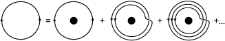
Figure 1: The free fermion contribution to $\Omega$. The conventional finite temperature Feynman diagram on the left is expanded as a sum over worldline loops about the compact time direction (“chronographs”) with winding number $\nu$ making a contribution proportional to $z^{\nu}$. The black dot indicates the nontrivial topology, and Euclidian time increases in the counterclockwise direction.

We will refer to the diagrams on the right in Fig. 1 as “chronographs”, which allow one to compute directly the $n^{th}$ term in the fugacity expansion of $\Omega$ or $\partial\Omega/\partial\mu$. The rules for chronographs can be easily generalized for computing the fugacity expansion in interacting systems: (i) Chronograph propagators ${\cal G}(\tau,{\mathbf{p}})$ can be defined in terms for the Minkowski propagator ${\widetilde{G}}^{M}(E,{\mathbf{p}})=i/(E-\varepsilon_{\mathbf{p}}+i\epsilon)$ at $\mu=0$ via the contour integral along the path $C$ shown in Fig 2, which simply picks up all the physical poles and cuts:

$${\cal G}(\tau,{\mathbf{p}})\equiv\theta(\tau-0^{+})\int_{C}\frac{dE}{2\pi}\,e^{-E\tau}\widetilde{G}^{M}(E,{\mathbf{p}})$$ (6)

${\cal G}$ should be thought of as a multi-valued function of $\tau$ living on a compact manifold of circumference $\beta$. For a free fermion, ${\cal G}_{0}(\tau,{\mathbf{p}})=-\theta(\tau)e^{-\tau\varepsilon_{\mathbf{p}}}$; (ii) vertices (from the Euclidian action) are located on the circle at Euclidian time $\tau_{i}$, each with a 3-momentum conserving $\delta$-function; (iii) one integrates over all vertex positions $\tau$ and all propagator 3-momenta ${\mathbf{p}}$; (iv) a factor of $(-1)^{\nu_{F}}$ is included where $\nu_{F}$ is the winding number carried by fermions in the diagram, with an additional $(-1)$ for each closed fermion loop in the parent Feynman diagram; (v) symmetry factors are computed as in Feynman diagrams, with the caveat that two propagators connecting the same two vertices do not warrant a symmetry factor when their length differs by $n\beta$; (vi) the winding number about compact Euclidian time, weighted by particle charge, is the order of the graph; all graphs of order $p$ are included in a fugacity expansion to order $z^{p}$. For example, a dimer loop with $\nu=1$ contributes to order $z^{2}$ since the dimer has particle number 2.

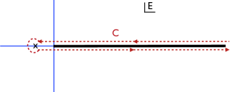
Figure 2: The contour $C$ in eq. (6) is designed to pick up contributions from all cuts and poles along the real energy axis.

III Interactions and $b_{2}$

To include 2-particle interactions it is convenient to represent the interaction not in terms of a potential, but by s-channel dimer exchange, a technique introduced in Kaplan (1997). The advantage is that the dimer — with a dispersion relation constructed to exactly reproduce the two particle phase shift $\delta$ — has a separable contact interaction with the fermions. This phase shift is assumed to be given, either directly from scattering data, or previously calculated from a potential model. That one can take this simplifying approach is due to the fact that the virial coefficients depend on interactions only through the $S$-matrix Dashen et al. (1969).

We focus on the case of s-wave scattering, commenting below on its generalization to other partial waves. Consider the Minkowski spacetime Lagrangian

$${\cal L}=\psi^{\dagger}(i\partial_{t}+\nabla^{2}/2M)\psi+\phi^{\dagger}K\phi+{\textstyle{\frac{1}{2}}}\phi^{\dagger}\psi^{T}\sigma_{2}\psi+\text{h.c.}$$ (7)

where $K$ is a function of the Galilean invariant operator $D=(i\partial_{t}+\nabla^{2}/4M)$. It is important to recognize that this is not a conventional effective field theory (EFT); in an EFT, one would perform a low energy expansion and express $K$ as a polynomial in $D$, as was done to subleading order in Kaplan (1997) and to leading order in Bedaque and Rupak (2003); such an expansion of $K$ in powers of $D$ corresponds directly to the effective range expansion of $p\cot\delta(p)$. However, here we consider $K$ to be a more general function of $D$ (e.g, nonlocal) chosen so that the full dimer Green’s function given by the sum in Fig. 3 results in the exact 2-fermion scattering amplitude:

$$\widetilde{G}^{M}_{\phi}(E,{\mathbf{P}}) = \frac{4\pi}{M}\frac{-i}{k\cot\delta(k)+\sqrt{-k^{2}}}\ ,$$ (8)

where $k^{2}=[M(E+2\mu)-{\mathbf{P}}^{2}/4+i\epsilon]$, $E$ and ${\mathbf{P}}$ being the total energy and momentum of the fermion pair. In Fig. 3 the geometric sum of loop diagrams creates the correct 2-fermion cut appearing as the $\sqrt{-k^{2}}$ term in the amplitude; the loops are linearly divergent, and the divergence is absorbed into a constant counterterm in $K$, so that the renormalized operator is $K_{R}=K-\text{const.}$ (see, for example Kaplan et al. (1998b, a)). This theory is valid beyond the radius of convergence of the effective range expansion, up to energies where inelastic processes set in, such as pion production in the case where the fermions are nucleons.

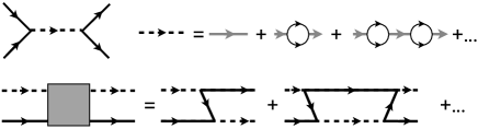
Figure 3: Feynman graphs for dimer mediated two-body scattering, and the integral equation relevant for three-body scattering (dashed line = fully dressed dimer, solid line = fermion; gray = $K^{-1}$).

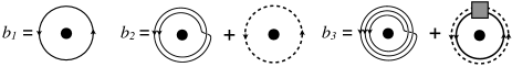
Figure 4: Chronograph expansion for the virial coefficients $b_{n}$. Dashed line: fully dressed dimer propagator, shaded box: summed three-body interaction from Fig. 3. For $b_{3}$, bosons or multiple fermion species would require introduction of a trimer field as well.

The chronographs in this theory for $b_{1,2,3}$ are shown in Fig. 4. The second coefficient $b_{2}$ gets the contribution $b_{2}^{(1)}=-1/4\sqrt{2}$ computed in eq. (5) from free fermions, as well as the dimer contribution computed from $\partial\Omega/\partial\mu$:

$$b_{2}^{(2)}=\frac{\lambda^{3}}{4}\int\frac{d^{3}{\mathbf{P}}}{(2\pi)^{3}}\int_{C}\frac{dE}{2\pi}e^{-\beta E}\widetilde{G}^{M}_{\phi}\frac{\partial(i{\widetilde{G}}^{M}_{\phi})^{-1}}{\partial\mu}\biggl{|}_{\mu=0}$$ (9)

where $\widetilde{G}^{M}_{\phi}$ and $k$ are given in eq. (8). The contour integration picks up contributions both from poles and from the cut along the positive real $E$ axis from $\sqrt{-k^{2}}$ in eq. (8). If the theory has bound states with binding energy $\varepsilon_{n}$, then $\widetilde{G}_{\phi}^{M}$ has poles at $E_{n}\equiv(\epsilon_{n}+{\mathbf{P}}^{2}/4M-2\mu)$ and the integrand in brackets has poles at $E=E_{n}$ with residue 2. To compute the contribution from the cut, one substitutes eq. (8) for $\widetilde{G}^{M}_{\phi}$ accounting for $\sqrt{-k^{2}}$ flipping sign across the cut. Combining the cut and pole contributions and performing the ${\mathbf{P}}$ integration we immediately recover the well-known result Beth and Uhlenbeck (1937); Pais and Uhlenbeck (1959)

$$b^{(2)}_{2}=\sqrt{2}\left[\sum_{n}e^{-\beta\epsilon_{n}}+\frac{1}{\pi}\int_{0}^{\infty}dk\,\frac{d\delta(k)}{dk}e^{-\beta\frac{k^{2}}{M}}\right]\ .$$ (10)

This analysis can be extended to other partial waves by introducing new dimer fields with appropriate couplings to fermions.

IV Computing $b_{3}$

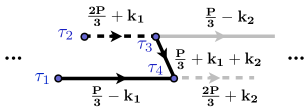
Figure 5: The three propagator subgraph (in black) contributing to $b_{3}$ and corresponding to the expression $L$ appearing in eqs. (11,12).

At third order we need to compute the new chronographs for $\Omega$ shown in Fig. 4, the first graph yielding the free fermion contribution, $b_{3}^{(1)}=1/9\sqrt{3}$ as computed in eq. (5). The second graph for $b_{3}^{(3)}$ sums all dimer-fermion and three fermion interactions, barring additional three-body forces; for a single species of fermion renormalizability does not require three-body forces and we shall ignore them here; however, in principle a trimer could be introduced to generate fundamental three-body forces. This diagram can be expressed in a loop expansion as

$$b_{3}^{(3)}=\lambda^{3}\sum_{n}{\rm Tr\,}\frac{L^{n}}{n}$$ (11)

where $L$ corresponds to the subdiagram in Fig. 5 with

$$\begin{aligned} &L_{12{\mathbf{k}}_{1},34{\mathbf{k}}_{2}}={\cal G}_{0}(\tau_{4}-\tau_{1},{\mathbf{P}}/3-{\mathbf{k}}_{1})\cr&\ \ \times{\cal D}(\tau_{3}-\tau_{2},2{\mathbf{P}}/3+{\mathbf{k}}_{1}){\cal G}_{0}(\tau_{4}-\tau_{3},{\mathbf{P}}/3+{\mathbf{k}}_{1}+{\mathbf{k}}_{2})\ ,\end{aligned}$$ (12)

${\cal G}_{0}$ being the fermion chronograph propagator and ${\cal D}$ being the dimer propagator computed from eqs. (6,8), and we include a symmetry factor of $1/n$, a spin factor of ${\rm Tr\,}\sigma_{2}^{2n}=2$ from the vertices and a factor of $(-1)$ due to $\nu_{F}=3$; there is no overall fermion sign from the parent Feynman diagram. In this expression, a product of $L$’s corresponds to the integral

$$L^{2}_{12{\mathbf{k}}_{1},56{\mathbf{k}}_{2}}=\int_{0}^{\beta}d\tau_{3}d\tau_{4}\int\frac{d^{3}{\mathbf{q}}}{(2\pi)^{3}}\,L_{12{\mathbf{k}}_{1},34{\mathbf{q}}}L_{34{\mathbf{q}},56{\mathbf{k}}_{2}}$$ (13)

with an integral over the center of mass momentum ${\mathbf{P}}$ implied in the trace; this ${\mathbf{P}}$ integral is gaussian and contributes a factor of $(3\sqrt{3}/\lambda^{3})$. Then the $n^{th}$ term in eq. (11) corresponds to the $(n+1)$-loop contribution to the last diagram in Fig. 4.

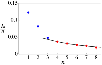
Figure 6: Results for $I_{n}/n$, including error estimate from numerical integration for $n=3,\ldots,8$. The solid line is the large-$n$ fit to the last five data points by the function $(c_{0}/n+c_{1}/n^{2})$, as described in the text.

At this point in order to be concrete we will narrow our focus to computing $b^{(3)}_{3}$ for unitary fermions, for which $p\cot\delta=0$ identically. From eqs. (6,8) we find the dimer propagator ${\cal D}(\tau,{\mathbf{q}})=-\theta(\tau)\sqrt{16\pi/M^{3}}\,e^{-\tau{\mathbf{q}}^{2}/4M}/\sqrt{\tau}$. In this case the expansion takes the form

$$b_{3}^{(3)}=3^{3/2}\sum_{n=1}^{\infty}\frac{(-1)^{n}I_{n}}{n}$$ (14)

where $I_{n}$ is given by the integral

$$\begin{aligned} &\left(16\pi\right)^{n/2}\int_{\cal T}\prod_{i=1}^{n}\frac{d\tau_{2i-1}d\tau_{2i}}{\sqrt{\tau_{2i+1}-\tau_{2i}}}\int\prod_{j=1}^{n}\frac{d^{3}{\mathbf{k}}_{j}}{(2\pi)^{3}}e^{-{\mathbf{k}}_{a}\cdot A_{ab}{\mathbf{k}}_{b}}\cr&={\left(2\pi\right)^{-n}}\int_{\cal T}\prod_{i=1}^{n}\frac{d\tau_{2i-1}d\tau_{2i}}{\sqrt{\tau_{2i+1}-\tau_{2i}}}\left(\det A\right)^{-\frac{3}{2}}\end{aligned}$$ (15)

which is positive and independent of $\beta$ and $M$, $A$ being the $n\times n$ matrix

$$\begin{aligned} A_{ab}&=\delta_{ab}\frac{4\tau_{2a+2}-\tau_{2a+1}+\tau_{2a}-4\tau_{2a-1}}{4}\cr&+\left(\hat{\delta}_{a,b+1}\frac{\tau_{2a}-\tau_{2a-1}}{2}+a\leftrightarrow b\right)\end{aligned}$$ (16)

with $\hat{\delta}_{ab}$ is the Kronecker $\delta$-function with indices defined modulo $n$, so that $\hat{\delta}_{n+a,b}=\hat{\delta}_{a,n+b}=\delta_{ab}$ for $1\leq a,b\leq n$, and $\int_{\cal T}$ represents a $2n$-dimensional time ordered integral over $\tau_{i}$ with $0\leq\tau_{1}\leq\tau_{2}<\ldots<\tau_{2n}\leq 1$ and $\tau_{2n+j}\equiv 1+\tau_{j}$ for $j=1,2$.

The integral $I_{n}$ can be performed analytically for $n=1,2$ with the result $I_{1}=2/(3\sqrt{3}\pi)$, $I_{2}=8/(9\sqrt{3}\pi)$; for $n=3,\ldots,8$ we have computed the integrals numerically. We find that $I_{n}$ is apparently a smooth function of $n$ for large $n$ and we perform a large-$n$ extrapolation, fitting our results for $n=4,\ldots,8$ to the function $I_{n}\sim(c_{0}+c_{1}/n)$ finding $c_{0}=0.1955\pm 0.0011$, $c_{1}=-0.1943\pm 0.0044$ (with highly correlated errors); the results are shown in Fig. 6. We estimate our errors by also fitting to the function $(c_{0}+c_{1}/n+c_{2}/n^{2})$, and varying the range of points used in the fit, finding a very stable result. Our final result for the interacting contribution to $b_{3}$ is $b_{3}^{(3)}=-0.3573\pm 0.0005$, or for the full answer, $b_{3}=-0.29315\pm 0.0005$, to be compared with the recent computation $b_{3}=-0.29095295$ by Liu, Hu and Drummond Liu et al. (2009), which involved summing over energy levels for three unitary fermions in a harmonic trap Werner and Castin (2006). It is remarkable that an expansion and extrapolation of chronographs is able to arrive at such a precise number for what is essentially a nonperturbative system; however, we do not have an explanation for why our procedure leads to an estimated error for $b_{3}$ ($\pm 0.0005$) which is significantly smaller than our discrepancy with Liu et al. ($0.0021$).

To our knowledge, this is the first time $b_{3}$ was calculated by analytical means for a strongly interacting system, and it suggests that the graphical techniques presented here for the virial expansion may prove powerful for applications to other systems as well.