Hydrophobic interactions with coarse-grained model for water

Abstract

Integral equation theory is applied to a coarse-grained model of water to study potential of mean force between hydrophobic solutes. Theory is shown to be in good agreement with the available simulation data for methane-methane and fullerene-fullerene potential of mean force in water; the potential of mean force is also decomposed into its entropic and enthalpic contributions. Mode coupling theory is employed to compute self-diffusion coefficient of water, as well as diffusion coefficient of a dilute hydrophobic solute; good agreement with molecular dynamics simulation results is found.

I Introduction

Hydrophobic interactions play an important role in a wide variety of phenomena, including collapse of hydrophobic polymers in water, micelle formation, and protein folding.berne09 ; pratt02 As a result, this problem has been actively studied theoretically.pratt77 ; lee84 ; watanabe86 ; smith93 ; ludemann96 ; ludemann97 ; garde01 ; shimizu01 ; ghosh02 ; huang03 ; rajamani05 ; choudhury05 ; li05 ; li05b ; howard08 ; chiu09 ; godawat09 ; athawale09 ; makowski10 ; setny10 ; chaimovich09 ; hammer10 The interactions between hydrophobic solutes in water have been investigated using both computer simulations and mean field theoretical methods. The former approach produces exact results for a given microscopic model, but at a significant computational cost, especially for large-size solutes, which require simulating a very large number of water molecules. The latter approach is much less computationally demanding, but inevitably involves approximations.

One possible way to reduce computational cost associated with simulation studies is to employ simplified coarse-grained solvent models.chiu09 ; chaimovich09 ; hammer10 Of particular relevance to the present study is the recent work of Shell and co-workers,chaimovich09 ; hammer10 who have shown that several thermodynamic and dynamic anomalies of pure water, as well as various features of hydrophobic interactions can be reasonably well reproduced with a coarse-grained water model based on an isotropic pairwise additive “Lennard-Jones plus Gaussian” (LJG) interaction potential. While the work of Shell and co-workers employed simulation-based techniques, their microscopic model based on an isotropic pair potential is ideally suited for approaches such as integral equation theory and mode-coupling theory (MCT), which would reduce computational expenses even further.egorov08b ; egorov08c ; egorov08e

Shell and co-workers have found that in order to properly reproduce the behavior of potential of mean force (PMF) between two hydrophobic solutes in water (e.g. its variation with the solvent temperature), the parameters of the coarse-grained LJG potential must be taken to be dependent on the thermodynamic state point of the solvent. Nevertheless, once the potential is parameterized for a given density and temperature of water, it can be employed to study the hydrophobic interactions between various solutes, and here is precisely where the computational efficiency of the integral equation approach could be very helpful. However, as mentioned above, the theory is necessarily approximate and its accuracy needs to be tested against the simulation data. The goal of the present study is to perform a comparison between theory and simulation in obtaining structural and dynamical properties of both pure water and dilute solutions of hydrophobic solutes.

The remainder of the paper is organized as follows. In Section II we present our microscopic model and theoretical methods for calculating structural, thermodynamic, and dynamical properties. The results are presented in Section III. Section IV concludes the paper.

II Microscopic Model and Theory

II.1 Microscopic Model

As a coarse-grained model for water, we consider a system comprised of spherical particles interacting via an isotropic LJG pair potential of the following form: chaimovich09 ; hammer10

$$\phi_{s}(r)=4\epsilon\left[\left(\frac{\sigma}{r}\right)^{12}-\left(\frac{\sigma}{r}\right)^{6}\right]+B\exp\left[-\frac{(r-r_{0})^{2}}{\Delta^{2}}\right],$$ (1)

where $\epsilon$ and $\sigma$ are the usual LJ parameters setting the energy and length scale of the interaction, while parameter $B$ sets the strength of the Gaussian term, whose center and width are determined by $r_{0}$ and $\Delta$, respectively.

In studying hydrophobic interactions, we consider dilute solutions, where solutes interact with solvent particles via isotropic pair potential $\phi(r)$ and with each other via another isotropic pair potential $\phi_{uu}(r)$, particular forms of these potentials depend on the solute and will be specified for each solute in Section III.

II.2 Structural Properties

We employ integral equation theory hansen86 to compute the solvent-solvent ($g_{s}(r)$) and the solute-solvent ($g(r)$) pair distribution functions and the solute-solute PMF ($W(r)$).

The starting point of the calculation is the Ornstein-Zernike relation between the solvent-solvent total ($h_{s}(r)=g_{s}(r)-1$) and direct ($c_{s}(r)$) pair correlation functions: hansen86

$$h_{s}(r)=c_{s}(r)+\rho\int d\vec{r}^{\,\prime}h_{s}(r^{\,\prime})c_{s}(|\vec{r}-\vec{r}^{\,\prime}|),$$ (2)

where $\rho$ is the bulk solvent number density. In order to solve the above equation, one needs an additional closure relation between $h_{s}(r)$ and $c_{s}(r)$. Here we employ thermodynamically self-consistent hybrid mean spherical approximation (HMSA) closure: zerah86

$$c_{s}(r)=\exp\{-\beta\phi_{s}(r)\}\left[1+\frac{\exp\left[f(r)\left(h_{s}(r)-c_{s}(r)\right)\right]-1}{f(r)}\right]-h_{s}(r_{1})+c_{s}(r_{1})-1,$$ (3)

where $\beta=1/k_{B}T$, and $f(r)=1-\exp(-\alpha r)$. Note that this closure interpolates between the soft-core mean spherical approximationmadden80 ($\alpha\rightarrow 0$) and the (hypernetted chain) HNC closure ($\alpha\rightarrow\infty$).zerah86

The value of the parameter $\alpha$ is determined by a thermodynamic consistency condition that is based on equating the isothermal compressibilities, $\chi_{T}^{v}$ and $\chi_{T}^{c}$, that follow respectively from the virial and compressibility routes: zerah86

$$(\rho kT\chi_{T}^{v})^{-1} = \left(\frac{\partial\beta P^{v}}{\partial\rho}\right),$$

$$(\rho kT\chi_{T}^{c})^{-1} = 1-\rho\int d\vec{r}c_{s}(r),$$ (4)

where the virial pressure $P^{v}$ is given by

$$\beta P^{v}=\rho-\frac{\beta\rho^{2}}{6}\int d\vec{r}r\phi^{\prime}_{s}(r)g_{s}(r),$$ (5)

with prime denoting differentiation with respect to the argument.

For an infinitely dilute solute in a solvent, the solute-solvent total ($h(r)=g(r)-1$) and direct ($c(r)$) pair correlation functions are also related via Ornstein-Zernike equation:

$$h(r)=c(r)+\rho\int d\vec{r}^{\,\prime}h(r^{\,\prime})c_{s}(|\vec{r}-\vec{r}^{\,\prime}|),$$ (6)

We employ the HNC closure to solve for $h(r)$ and $c(r)$:

$$h(r)=\exp[-\beta\phi(r)+h(r)-c(r)]$$ (7)

The accuracy of this approach will be tested in the next Section by comparing theoretical results with simulations.

Finally, for two dilute solutes in a solvent, the solute-solute PMF is composed of two terms:

$$W(R)=\phi_{uu}(R)+\Delta W(R),$$ (8)

where the first term is the bare solute-solute interaction potential, while the second term is the solvent-mediated PMF given by the following exact relations: egorov01c

$$\Delta W(R)=\int_{R}^{\infty}F(R^{\,\prime})dR^{\,\prime},$$ (9)

where the excess mean force, $F(R)$, is given by:

$$\vec{F}(R)=-\int d\vec{r}{{~{}}}\nabla\phi(r)\rho(\vec{r};R).$$ (10)

In the above, $\rho(\vec{r};R)$ is the conditional probability of finding the solvent particle at $\vec{r}$ given that one solute is at the origin, and the other solute is located at $\vec{R}$. We compute this conditional probability from the anisotropic HNC closure, which has been thoroughly tested against computer simulations in our earlier work: egorov01c ; egorov02e

$$\rho(\vec{r};R)=\rho\exp\left[-\beta\left(\phi(r)+\phi(|\vec{r}-\vec{R}|)\right)+\int d\vec{r}^{\,\prime}c(|\vec{r}-\vec{r}^{\,\prime}|)(\rho(\vec{r}^{\,\prime};R)-\rho)\right].$$ (11)

From the solute-solute PMF one can easily obtain the solute-solute radial distribution function given by:

$$g_{uu}(R)=\exp(-\beta W(R)).$$ (12)

As will be seen from the results presented below, for a typical hydrophobic solute such as methane, the solute-solute PMF typically displays two pronounced minima corresponding to the contact pair and the solvent-separated pair of the solutes.ludemann96 ; ghosh02 Concomitantly, the solute-solute radial distribution function is characterized by two corresponding maxima, with the second maximum (corresponding to the solvent-separated pair) bracketed by two minima located at $R_{1}$ and $R_{2}$. In what follows, we will study the dependence of the methane-methane PMF and $g_{uu}(R)$ on the water density and temperature. In order to characterize the behavior of these functions by a single parameter, we will compute the equilibrium constant for the conversion of the contact pair into the solvent-separated pair:ludemann96

$$K_{eq}=\frac{\int_{0}^{R_{1}}g_{uu}(r)r^{2}dr}{\int_{R_{1}}^{R_{2}}g_{uu}(r)r^{2}dr}.$$ (13)

II.3 Dynamical Properties

We employ the MCT-based approach to compute the self-diffusion coefficient of the pure water, as well as the diffusion coefficient of a dilute solute. In this approach, the self-diffusion coefficient is obtained from the total friction $\zeta$:balucani94 ; bhattacharyya98 ; egorov03b

$$D=\frac{k_{B}T}{m_{s}\zeta},$$ (14)

where $m_{s}$ is the mass of the water molecule, and the MCT expression for $\zeta$ is comprised of binary and collective density contributions:bhattacharyya97

$$\zeta=\zeta_{b}+\zeta_{\rho\rho}$$ (15)

In what follows, we will be calculating self-diffusion coefficient at relatively high water densities, and therefore we neglect the hydrodynamic contribution to friction which arises from the coupling of the tagged solvent particle motion to the collective transverse current mode.bhattacharyya97

The binary term is given by the total time integral of the fast decaying binary component of the time dependent friction, which we model as a Gaussian function, whose parameters are chosen to reproduce the exact short-time behavior of the total time-dependent friction, $\zeta(t)$, up to the term of order $t^{2}$:balucani94

$$\zeta_{b}(t)=\zeta(0)\exp\left[\frac{\ddot{\zeta}(0)t^{2}}{2\zeta(0)}\right],$$ (16)

with the initial-time value given by:

$$\zeta(0)=\frac{4\pi\rho}{3m_{s}}\int_{0}^{\infty}drr^{2}g_{s}(r)\nabla^{2}\phi_{s}(r).$$ (17)

The zero-time value of the second time derivative, $\ddot{\zeta}(0)$, can be similarly obtained from the fluid intermolecular potential and radial distribution function.egorov03b ; balucani94

The density term arises from the coupling of the tagged solvent particle motion to the collective density mode:bhattacharyya97

$$\zeta_{\rho\rho}=\int_{0}^{\infty}\zeta_{\rho\rho}(t)dt,$$ (18)

with

$$\zeta_{\rho\rho}(t)=\frac{k_{B}T\rho}{6\pi^{2}m_{s}}\int_{0}^{\infty}dkk^{4}c_{s}(k)^{2}\left[F_{s}(k,t)F(k,t)-F_{s}^{0}(k,t)F^{0}(k,t)\right]$$ (19)

where $F(k,t)$ is the solvent dynamic structure factor, $F_{s}^{0}(k,t)=\exp(-k_{B}Tk^{2}t^{2}/2m_{s})$, and $F_{s}(k,t)$ is the solvent self-dynamic structure factor, for which we have adopted a simple Gaussian model:balucani94 ; bhattacharyya97

$$F_{s}(k,t)=\exp\left[\frac{-k_{B}Tk^{2}}{m_{s}\zeta}\left(t+\frac{1}{\zeta}(e^{-t\zeta}-1)\right)\right].$$ (20)

We obtain the solvent dynamic structure factor from the continued fraction representation of its Laplace transform truncated at the second order:balucani94

$$F(k,z)=\frac{S(k)}{z+\frac{\displaystyle{\delta_{1}(k)}}{\displaystyle{z+}\frac{\displaystyle{\delta_{2}(k)}}{\displaystyle{z+}\displaystyle{\tau^{-1}(k)}},}}$$ (21)

where $\delta_{i}(k)$ is the initial time value of the $i^{\mbox{th}}$ order memory function (MF) of $F(k,t)$. For the parameter $\tau^{-1}(k)$ we use the expression due to Lovesey:lovesey71 $\tau^{-1}(k)=2\sqrt{\delta_{2}(k)/\pi}$. The quantities $\delta_{1}(k)$ and $\delta_{2}(k)$ can be easily calculated from the first three short-time expansion coefficients of $F(k,t)$; the microscopic expressions for the latter are well-known and will not be reproduced here.hansen86 ; balucani94 ; bansal77

Given that the self-dynamic structure factor in Eq. (20) is a function of $\zeta$, which, in turn, depends on $F_{s}(k,t)$ via Eq. (18) and (19), the above set of MCT equations for $\zeta$ needs to be solved iteratively and self-consistently. One could use a more accurate model for $F_{s}(k,t)$ in terms of the velocity time correlation function of a tagged fluid particle,bhattacharyya98 but our numerical calculations have shown that this does not change the results for $D$ in a noticeable way.

The diffusion coefficient of a dilute solute is obtained in the same way as the solvent self-diffusion coefficient, with the understanding that in the above set of MCT equations $\phi_{s}(r)$, $g_{s}(r)$, and $c_{s}(r)$ are replaced with $\phi(r)$, $g(r)$, and $c(r)$, respectively. Additionally, $F_{s}(k,t)$ now has the meaning of the solute self-dynamic structure factor, and $F_{s}^{0}(k,t)=\exp(-k_{B}Tk^{2}t^{2}/2m)$ is its inertial component, where $m$ is the solute mass. Finally, $m_{s}$ is replaced with $m$ in Eqs. (14), (17), (19), and (20).

In the next section, we compare our theoretical results for structural and dynamical properties of pure water and dilute solutions of hydrophobic solutes with MD data and analyze the dependence of various computed properties on the solvent thermodynamic conditions.

III Results

III.1 Pure Water

We start by presenting our results for the structural and dynamical properties of pure water. Parameters entering the LJG potential given by Eq. (1) are dependent on density and temperature and are taken from Ref. chaimovich09, , where they were obtained from the relative entropy optimization method. In Fig. 1 we compare simulation results for the oxygen-oxygen radial distribution function of all-atom SPC/E water,athawale09 and the HMSA result for $g_{s}(r)$ of coarse-grained water described by the LJG potential. The two distribution functions are generally in good agreement except some discrepancies in the range between 3 and 6 Å. The same discrepancies were seen in the earlier comparison of simulated $g_{s}(r)$ for SPC and LJG water, i.e. if one were to compare HMSA theory with simulations done for the coarse-grained LJG water (not shown), the two distribution functions would be nearly indistinguishable.

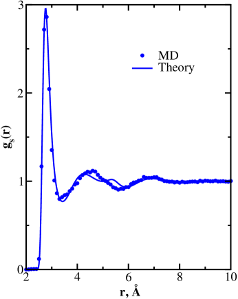
Figure 1: Radial distribution function of pure water at T=300 K and $\rho$=1 g/cm³. Symbols are the simulation results for the oxygen-oxygen radial distribution function of all-atom SPC/E water,athawale09 and the line is from HMSA theory for coarse-grained water described by the LJG potential.

The same level of agreement between theoretical and simulation results for the structural properties of coarse-grained water is obtained at other thermodynamic conditions, as can be seen from Fig. 2a, where we present MDchaimovich09 (symbols) and HMSA (lines) pressure isochores for two values of water density: $\rho$=0.9 g/cm³ and 1 g/cm³, with theoretical results obtained from Eq. (5).

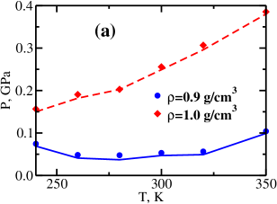
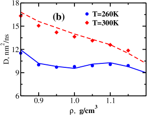
Figure 2: (a)Pressure isochores for the coarse-grained LJG water model; symbols are from MD simulations,chaimovich09 and lines are from the HMSA integral equation theory. (b) Self-diffusion coefficient of the coarse-grained LJG water as a function of density along two isotherms; symbols are from MD simulations,chaimovich09 and lines are from the MCT approach.

One sees that the HMSA results for pressure are in excellent agreement with the MD data for both isochores throughout the entire temperature range studied, thereby confirming the accuracy of the theory in providing structural information for the coarse-grained water model. In particular, theory successfully reproduces the characteristic anomalous water behavior, with pressure decreasing as a function of $T$ along the isochore $\rho$=0.9 g/cm³ at the lower end of the temperature range studied, subsequently passing through a minimum, and then growing with temperature.

Having ascertained the accuracy of the HMSA theory in calculating structural and thermodynamic properties of pure water, we next use the structural data as input to compute water self-diffusion coefficient from the MCT approach. In Fig. 2b we present simulationchaimovich09 (symbols) and theoretical (lines) results for self-diffusion coefficient of the coarse-grained LJG water as a function of density along two isotherms: T=260 K and T=300 K. At the higher temperature, the self-diffusion coefficient decreases monotonically with increasing density, while at the lower temperature, anomalous behavior is observed, where the self-diffusion coefficient passes through a minimum around $\rho$=1.0 g/cm³, increases with density between 1.0 and 1.1 g/cm³, passes through a maximum, and then decreases with density. One sees that theory is in good agreement with simulation for both isotherms, and in particular captures the characteristic water diffusion anomaly well.

Having considered structural, thermodynamic, and dynamic properties of pure coarse-grained LJG water, we next turn to dilute solutions of hydrophobic solutes in LJG water.

III.2 Methane Solutes in Water

For the purpose of modeling dilute solution of methane in water, we have employed LJ potentials for both solute-solvent and solute-solute interactions:

$$\phi(r)=4\epsilon_{us}\left[\left(\frac{\sigma_{us}}{r}\right)^{12}-\left(\frac{\sigma_{us}}{r}\right)^{6}\right],$$ (22)

and

$$\phi_{uu}(r)=4\epsilon_{uu}\left[\left(\frac{\sigma_{uu}}{r}\right)^{12}-\left(\frac{\sigma_{uu}}{r}\right)^{6}\right].$$ (23)

In order to compare our theoretical results with the earlier simulation study of methane solution in LJG water,chaimovich09 ; athawale09 we have chosen the same values of $\epsilon$ and $\sigma$ parameters as in the simulations: $\sigma_{us}$=3.45 Å, $\epsilon_{us}$=0.89 kJ/mol, $\sigma_{uu}$=3.73 Å, and $\epsilon_{uu}$=1.23 kJ/mol.

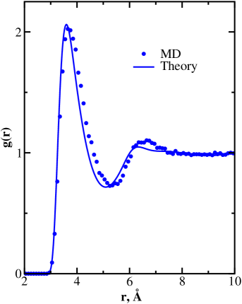
Figure 3: Methane-water radial distribution function at T=300 K and $\rho$=1 g/cm³. Symbols are the simulation results for the methane-water radial distribution function with all-atom SPC/E water,athawale09 and the line is from HNC theory for coarse-grained water described by the LJG potential.

In Fig. 3 we compare simulation results for the methane-water radial distribution function with all-atom SPC/E water,athawale09 and the HNC result for $g(r)$ with coarse-grained LJG water. The two distribution functions are generally in good agreement except some discrepancies in the range between 4 and 7 Å. As in the case of pure water, the agreement would be significantly better if one were to compare theory with simulation performed for methane in coarse-grained LJG water.

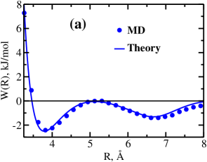
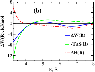
Figure 4: (a)PMF between two dilute methane solutes in coarse-grained LJG water; symbols are from MD simulations,chaimovich09 and lines are from the integral equation theory. (b) Solvent-mediated PMF between two dilute methane solutes in coarse-grained LJG water; also shown are entropic and enthalpic terms.

This is confirmed by comparing theoretical and simulation results for the PMF between two dilute methane solutes in LJG water, which are presented in Fig. 4a for thermodynamic state point T=300 K and $\rho$=1 g/cm³. One sees that theory is in excellent agreement with simulation throughout the entire range of separations between the two methane solutes, indicating that it accurately reproduces the anisotropic density distribution of LJG water molecules around two methane solutes at all separations considered. In particular, theory properly reproduces the locations and the depths of the two minima in the PMF – the first one corresponding to the contact pair (located around 3.9 Å), and the second one corresponding to the solvent-separated pair (located around 6.7 Å); the contact pair minimum is deeper compared to the solvent-separated one.

The agreement is equally good at the other two temperatures for which simulations were performed: T=280 K and T=320 K (not shown). On the basis of this information, we have decomposed the solvent-mediated PMF given by the integral equation theory into enthalpic and entropic contributions:smith93 ; ghosh02

$$\Delta S(T)\approx\frac{\Delta W(T+\Delta T)-\Delta W(T-\Delta T)}{2\Delta T},$$ (24)

and

$$\Delta H=\Delta W+T\Delta S,$$ (25)

where $\Delta T$=20 K in our calculations. The corresponding results are presented in Fig. 4b. In agreement with previous simulation results,ghosh02 one sees that the solvent-mediated PMF at the location of the contact pair minimum is completely dominated by the entropic contribution, with enthalpic term very close to zero but slightly unfavorable (positive). At larger separations, the enthalpic contribution becomes favorable and the entropic term unfavorable; the solvent-mediated PMF at the location of the solvent-separated pair minimum is dominated by the enthalpic contribution.ghosh02

In order to present our results for methane-methane PMF at other densities and temperatures in a compact form, we have computed the equilibrium constant for the conversion of the contact pair into the solvent-separated pair from Eq. (13). Theoretical results for $K_{eq}$ along two isotherms are presented in Fig. 5 together with the only simulation data point availablechaimovich09 at T=300 K and $\rho$=1 g/cm³.

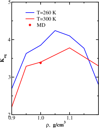
Figure 5: Theoretical results for the equilibrium constant for the conversion of the contact pair into the solvent-separated pair along two isotherms.

One sees that in agreement with earlier simulation work,ludemann96 the solvent-separated pair is more stable in terms of $K_{eq}$ at all densities and temperatures studied. For both isotherms, the equilibrium constant first increases with density, passes through a maximum between 1.05 g/cm³ and 1.1 g/cm³, and then decreases with density. Except for the highest density considered ($\rho$=1.2 g/cm³), the equilibrium constant is larger at the lower temperature.

III.3 Fullerenes in Water

For the purpose of modeling dilute solution of fullerenes in water, we have employed the following form for the solute-solvent interaction potential:girifalco00

$$\phi(r)=4N\epsilon_{us}\frac{\sigma_{us}^{2}}{rR}\left(\frac{1}{20}\left[\left(\frac{\sigma_{us}}{R-r}\right)^{10}-\left(\frac{\sigma_{us}}{R+r}\right)^{10}\right]-\frac{1}{8}\left[\left(\frac{\sigma_{us}}{R-r}\right)^{10}-\left(\frac{\sigma_{us}}{R+r}\right)^{10}\right]\right),$$ (26)

where $N$=60, R=3.55 Å, $\sigma_{us}$=3.19 Å, and $\epsilon_{us}$=0.392 kJ/mol.li05b

The fullerene-fullerene direct interaction potential is given by:girifalco00

$$\phi_{uu}(r)=-\alpha\left[\frac{1}{s(s-1)^{3}}+\frac{1}{s(s+1)^{3}}-\frac{2}{s^{4}}\right]+\beta\left[\frac{1}{s(s-1)^{9}}+\frac{1}{s(s+1)^{9}}-\frac{2}{s^{10}}\right],$$ (27)

where $\alpha$=4.4775 kJ/mol, $\beta$=0.0081 kJ/mol, and $s=r/2R$.

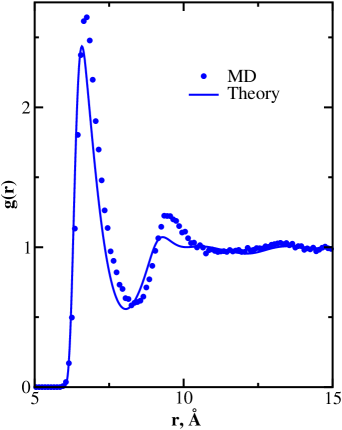
Figure 6: Fullerene-water radial distribution function at T=300 K and $\rho$=1 g/cm³. Symbols are the simulation results for the fullerene-water radial distribution function with all-atom SPC/E water,athawale09 and the line is from HNC theory for coarse-grained water described by the LJG potential.

In Fig. 6 we compare simulation results for the fullerene-water radial distribution function with all-atom SPC/E water,athawale09 and the HNC result for $g(r)$ with coarse-grained LJG water. The agreement between the two distribution functions is satisfactory in general, although theory underestimates the heights of both primary and secondary peaks of $g(r)$. Somewhat surprisingly, these discrepancies do not manifest themselves in the results for the solvent-mediated potential of mean force between two dilute fullerenes, as can be seen from Fig. 7, where we present simulationli05b and theoretical results for $\Delta W(R)$. Theory and simulation are in good agreement throughout the entire range of separations studied, which could be a result of fortuitous cancellation of errors.

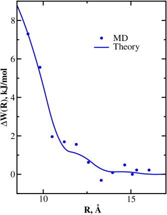
Figure 7: Solvent-mediated PMF between two dilute fullerene solutes in water. Symbols are the simulation results,li05b and lines are from integral equation theory.

In addition to the structural aspects of fullerene hydration, we have also studied dynamics of fullerene solutes in water. In particular, we have used the MCT approach outlined in the previous section to compute the diffusion coefficient of fullerene in water at thermodynamic state point T=300 K and $\rho$=1 g/cm³; we have obtained the value $D$=1.73 nm²/ns. This can be compared to the simulation resultcolherinhas11 of $D$=1.9 $\pm$ 0.4 nm²/ns, i.e. theoretical value is within the error-bars of the simulation result.

IV Conclusion

In this paper we have performed a theoretical study of structural, thermodynamic, and dynamic properties of a coarse-grained water model based on a spherically symmetric LJG pair potential. For pure water, thermodynamically self-consistent HMSA integral equation theory was shown to give accurate results for microstructure and thermodynamics, while MCT theory was in good agreement with the simulation data for the self-diffusion coefficient, including its anomalous density dependence.

In studying the structure of dilute solutions of hydrophobic solutes, anisotropic HNC theory was used to calculate the solute-solute PMF and the equilibrium constant for the conversion of the contact pair into the solvent-separated pair. Theory was shown to be in good agreement with the available simulation data for both methane-methane and fullerene-fullerene PMF. It would be of interest to extend our theoretical approach to larger solutes, such as graphene plates;howard08 this will be the subject of future research.

V Acknowledgment

The author would like to thank Profs. M. S. Shell and S. Garde, and Drs. A. Chaimovich and S. N. Jamadagni for sending the simulation data.

References

- (1) B. J. Berne, J. D. Weeks, and R. H. Zhou, Annu. Rev. Phys. Chem. 60, 85 (2009)
- (2) L. R. Pratt, Annu. Rev. Phys. Chem. 53, 409 (2002)
- (3) L. R. Pratt and D. Chandler, J. Chem. Phys. 67, 3683 (1977)
- (4) C. Y. Lee, J. A. McCammon, and P. J. Rossky, J. Chem. Phys. 80, 4448 (1984)
- (5) K. Watanabe and H. C. Andersen, J. Phys. Chem. 90, 795 (1986)
- (6) D. E. Smith and A. D. J. Haymet, J. Chem. Phys. 98, 6445 (1993)
- (7) S. Lüdemann, H. Schreiber, R. Abseher, and O. Steinhauser, J. Chem. Phys. 104, 286 (1996)
- (8) S. Lüdemann, R. Abseher, H. Schreiber, and O. Steinhauser, J. Am. Chem. Soc. 119, 4206 (1997)
- (9) S. Garde and H. S. Ashbaugh, J. Chem. Phys. 115, 977 (2001)
- (10) S. Shimizu and H. S. Chan, J. Chem. Phys. 115, 3424 (2001)
- (11) T. Ghosh, A. E. Garcia, and S. Garde, J. Chem. Phys. 116, 2480 (2002)
- (12) X. Huang, C. J. Margulis, and B. J. Berne, J. Phys. Chem. B 107, 11742 (2003)
- (13) S. Rajamani, T. M. Truskett, and S. Garde, Proc. Natl. Acad. Sci. USA 102, 9457 (2005)
- (14) N. Choudhury and B. M. Pettitt, J. Am. Chem. Soc. 127, 3556 (2005)
- (15) L. Li, D. Bedrov, and G. D. Smith, J. Chem. Phys. 123, 204504 (2005)
- (16) L. Li, D. Bedrov, and G. D. Smith, Phys. Rev. E 71, 011502 (2005)
- (17) J. J. Howard, J. S. Perkyns, N. Choudhury, and B. M. Pettitt, J. Chem. Theory Comput. 4, 1928 (2008)
- (18) C. C. Chiu, P. B. Moore, W. Shinoda, and S. O. Nielsen, J. Chem. Phys. 131, 244706 (2009)
- (19) R. Godawat, S. N. Jamadagni, and S. Garde, Proc. Natl. Acad. Sci. USA 106, 15119 (2009)
- (20) M. V. Athawale, S. N. Jamadagni, and S. Garde, J. Chem. Phys. 131, 115102 (2009)
- (21) M. Makowski, C. Czaplewski, A. Liwo, and H. A. Scheraga, J. Phys. Chem. B 114, 993 (2010)
- (22) P. Setny, R. Baron, and J. A. McCammon, J. Chem. Theory Comput. 6, 2866 (2010)
- (23) A. Chaimovich and M. S. Shell, Phys. Chem. Chem. Phys. 11, 1901 (2009)
- (24) M. U. Hammer, T. H. Anderson, A. Chaimovich, M. S. Shell, and J. Israelachvili, Faraday Discuss. 146, 1 (2010)
- (25) S. A. Egorov, J. Chem. Phys. 128, 144508 (2008)
- (26) S. A. Egorov, J. Chem. Phys. 128, 174503 (2008)
- (27) S. A. Egorov, J. Chem. Phys. 129, 024514 (2008)
- (28) J. P. Hansen and I. R. McDonald, Theory of Simple Liquids, 2nd ed. (Academic, London, 1986)
- (29) G. Zerah and J.-P. Hansen, J. Chem. Phys. 84, 2336 (1986)
- (30) W. G. Madden and S. A. Rice, J. Chem. Phys. 72, 4208 (1980)
- (31) E. Rabani and S. A. Egorov, J. Chem. Phys. 115, 3437 (2001)
- (32) E. Rabani and S. A. Egorov, Nanoletters 2, 69 (2002)
- (33) U. Balucani and M. Zoppi, Dynamics of the Liquid State (Clarendon, Oxford, 1994)
- (34) S. Bhattacharyya and B. Bagchi, J. Chem. Phys. 109, 7885 (1998)
- (35) S. A. Egorov, J. Chem. Phys. 119, 4798 (2003)
- (36) S. Bhattacharyya and B. Bagchi, J. Chem. Phys. 106, 1757 (1997)
- (37) S. W. Lovesey, J. Phys. C. 4, 3057 (1971)
- (38) R. Bansal and K. N. Pathak, Phys. Rev. A 15, 2519 (1977)
- (39) L. A. Girifalco, M. Hodak, and R. S. Lee, Phys. Rev. B 62, 13104 (2000)
- (40) G. Colherinhas, T. L. Fonseca, and E. E. Fileti, Carbon 49, 187 (2011)