Abstract

Recently, to explain the origin of neutrino masses a model based on confining some hidden fermionic bound states into right-handed chiral neutrinos has been proposed. One of the consequences of condensing the hidden sector fields in this model is the presence of sterile composite Dirac neutrinos of keV mass, which can form viable warm dark matter particles. We have analyzed constraints on this model from the observations of satellite based telescopes to detect the sterile neutrinos in clusters of galaxies.

Keywords: Dirac neutrino masses, Dirac sterile neutrinos, warm dark matter, X-rays, Galaxy clusters

1 Introduction

Since the discovery of neutrino oscillations in the solar [1] and atmospheric [2] neutrino experiments, neutrinos have played a vital role in the extension of standard model. Although gauge hierarchy problem is the major motivation for physics beyond the standard model, the tiny masses of neutrinos can guide the model building part of new physics in the neutrino sector. Theoretically, the neutrinos can be either Dirac or Majorana fields, depending on if lepton number is conserved or not in nature. In the literature, models which explain the tiny neutrino mass scale of 0.1 eV are mostly based on the seesaw mechanism [3] which requires lepton number violating Majorana neutrinos. A test for the Majorana neutrinos is the existence of neutrinoless double beta decay process, which has not been found in the experiments conducted so far. In the light of this, models based on Dirac neutrinos have also been proposed [4]. Recently, in a model known as composite Dirac neutrinos [5], Dirac neutrino masses have been proposed by conceiving right-handed neutrinos as composed objects of hidden fermionic chiral bound states at a high scale $\Lambda$ [6, 7]. The hidden chiral bound states and standard model fields arise due to confinement of an ultraviolet preonic theory at another higher scale $M\gg\Lambda$. The gauge symmetries of the hidden sector and the standard model can be broken in such a way that in the low energy regime a gauge symmetry is left unbroken which could be equivalent to the gauged U(1)_B-L, and hence in this model only Dirac neutrino masses arise. The neutrino masses in this model come out to be tiny due to the suppression factor of $\Lambda/M$. One of the phenomenological consequences of this model is that at the scale $\Lambda$, apart from chiral right-handed neutrinos non-chiral sterile neutrinos can be produced due to confinement. The mass scale $m_{s}$ of these sterile neutrinos depend on the nature of confinement, and thus on both $M$ and $\Lambda$. In a particular case and for suitable values of $M$ and $\Lambda$ its mass scale is $m_{s}\sim$ keV, which is the right amount to form a warm dark matter particle [8]. These sterile states have small mixing with active neutrinos, which is roughly $\theta\approx m_{\nu}/m_{s}$, $m_{\nu}$ being the light active neutrino mass scale.

The existence of dark matter in the universe is well established by galactic rotation curves, cosmic microwave background radiation and gravitational lensing. The nature of dark matter is unknown, yet about 20$\%$ of the universe is filled with it. The issue of dark matter is another compelling reason for the extension of standard model. Sterile neutrinos, which are gauge singlets, have been thought to be good warm dark matter particles [8]. These fields exist in many extensions of the standard model, one of them is the composite Dirac neutrino model which is described in the previous paragraph. Provided the mixing angle $\theta$ between sterile and active light neutrinos is sufficiently small, the leading decay life time for keV mass sterile states into three active neutrinos can be larger than the age of the universe, thus making them perfect dark matter candidates. One of the major channels to detect a sterile neutrino is its one-loop decay into photon and an active neutrino. For a keV mass sterile neutrino the emitted photon energy would be in the X-ray region, and this decay feature can be seen in the diffuse X-ray background of the universe or in the X-ray flux from a cluster of galaxies. There would be continuum X-ray background from a cluster of galaxies, nevertheless, the signal from a photon due to sterile neutrino decay should be a sharp peak on top of the X-ray background.

Satellite based experiments like Chandra, XMM-Newton, etc have been operated to detect the decay line feature of photon due to sterile neutrinos in the clusters of galaxies and also in the diffuse X-ray background. The null results of this search put exclusion area in the plane of sterile neutrino mass $m_{s}$ and the mixing angle $\theta$ [9, 10, 11, 12, 13]. As described above, in the composite Dirac neutrino model the sterile neutrino mass and the mixing angle are related to the confinement scales $M$ and $\Lambda$ in such a way to provide a viable warm dark matter particle and also a natural mechanism for neutrino masses. The negative results of the above mentioned experiments on the sterile neutrino decay can put constraints on the composite scales $M$ and $\Lambda$. In the original paper [5], order of magnitude estimations have been made on the model parameters to explain the neutrino masses and dark matter. In this work we study quantitative constraints on the parameters $(\Lambda,M)$ of the composite Dirac neutrino model due to these various X-ray based experiments.

The paper has been organized as follows. In the next section we give a brief overview on the composite Dirac neutrino model. In Sec. 3 we describe about some X-ray based experiments and their findings. We apply these results in the specified composite Dirac neutrino model and present the constraints on the model parameters $(\Lambda,M)$. We conclude in Sec. 4.

2 Composite Dirac Neutrino model

This model assumes an ultraviolet (UV) preonic theory which confines into standard model and hidden sector fields at a high scale $M$ [5, 6]. The symmetry of this theory spontaneously breaks into $G_{c}\otimes G_{F}\otimes G_{\rm SM}$ at the scale $M$. Here $G_{c}$, $G_{F}$ and $G_{\rm SM}$ are confinement, flavor and standard model gauge symmetries, respectively. Below the scale $M$ the necessary fields in our context are the following: (a) standard model lepton doublets $L$ which are $G_{c}\otimes G_{F}$ singlets; (b) hidden fermionic chiral bound states $q$, which are singlets under $G_{\rm SM}$ but charged under $G_{c}\otimes G_{F}$; (c) scalar condensate $\phi$ which transforms as doublet under the electroweak group of $G_{\rm SM}$, charged under $G_{F}$ and singlet under $G_{c}$. The condensate $\phi$ can be interpreted as Higgs doublet of the standard model. Now, consider a combination of $n$ hidden chiral bound states as $q^{n}$. Imagine that the charges of $\phi$ and $q^{n}$ are arranged in such a way that $\phi^{*}q^{n}$ is a singlet under $G_{c}\otimes G_{F}$. Then, in the effective field theory below the scale $M$ there can be an irrelevant operator in the Lagrangian of the form

$${\cal L}=\frac{\lambda}{M^{3(n-1)/2}}\bar{L}\tilde{\phi}q^{n},$$ (1)

where $\tilde{\phi}=-i\sigma_{2}\phi^{*}$, $\sigma_{i}$ are the Pauli matrices. The hidden sector of this model can undergo one more confinement at a scale $\Lambda$ much below the scale $M$, thereby condensing the $q^{n}$ into a right-handed bound state $N_{R}$ as

$$q^{n}\to N_{R}\Lambda^{3(n-1)/2}.$$ (2)

Since the bound states are fermionic particles, $n$ should be odd and $n\geq 3$. Plugging eq. (2) into eq. (1), in the low energy regime one gets

$${\cal L}=\lambda\left(\frac{\Lambda}{M}\right)^{3(n-1)/2}\bar{L}\tilde{\phi}N_{R},$$ (3)

The compound field $q^{n}$ is supposed to contain a right-handed spin-1/2 Lorentz representation, and hence the field $N_{R}$, which forms due to condensation below $\Lambda$, can be interpreted as chiral right-handed neutrino. We get Dirac neutrino masses for neutrinos from the above equation after electroweak symmetry breaking. The mass scale of these neutrinos can be of order 0.1 eV by appropriately choosing the suppression factor $\epsilon=\frac{\Lambda}{M}$ for $\lambda\sim{\cal O}(1)$. Let us note in passing that composite Majorana neutrinos have also been studied with a mini-seesaw mechanism for neutrino masses [14].

In the previous paragraph we have given the essential idea of explaining the smallness of neutrino masses by conceiving all the standard model fields in the low energy theory arising as condensates of high energy UV preonic theory. An important point to note here is that the masses of sterile neutrinos depend on the type of interactions of the fermionic bounds states, from which they are formed. If these fermionic bound states are gauge singlets interacting with scalar condensates via heavy gauge bosons or massive scalars at the energy scale $M$, then the sterile neutrinos acquire masses at loop level and their mass scale would be suppressed to $m_{s}\sim\frac{\Lambda^{3}}{M^{2}}$. This procedure has been dubbed as secondary mass generation mechanism [5, 15].

At the confinement scale $\Lambda$ the symmetry $G_{c}\otimes G_{F}$ breaks into $G^{\prime}_{c}\otimes G^{\prime}_{F}$. All chiral bound states are $G^{\prime}_{c}$ singlets but transforms under $G^{\prime}_{F}$. A simple choice for the $G^{\prime}_{F}$ is $U(1)_{F}$. The charges of the fields $L$, $\phi$ and $N_{R}$ can be chosen under $U(1)_{F}$ in such a way that after the electroweak symmetry breaking a gauge symmetry $U(1)_{a}$, which is an axial combination of the hypercharge group $U(1)_{Y}$ and $U(1)_{F}$, is left unbroken. It can be shown that the symmetry $U(1)_{a}$ is equivalent to lepton number [5]. Hence, in this model lepton number is conserved and only Dirac neutrino mass terms exist.

A detailed model by including mass terms for quarks and leptons has been constructed in [5] with the choice $G^{\prime}_{F}$ = $U(1)_{F}$. It has been shown that the axial combination of $U(1)_{Y}$ and $U(1)_{F}$ would be isomorphic to $U(1)_{B-L}$, which remains as an exact symmetry after electroweak symmetry breaking. Moreover, the charges assigned under $U(1)_{F}$ satisfy requirements for the cancellation of anomalies in this model. In general, at the confinement scale $\Lambda$ some number of right-handed bound states $N_{R}^{I}$, $I=1,\cdots,N$, can be produced. Out of which, $I=i=1,2,3$ should be chiral right-handed neutrinos in order to give masses to three neutrinos through mass terms of the form of eq. (3). The remaining $I=\alpha=4,\cdots,N$ can form vector-like singlet neutrinos, for which the left-handed components $N_{L}^{\alpha}$ exist at the confinement scale $\Lambda$. The fields $N_{L}^{\alpha},N_{R}^{\alpha}$ are by nature sterile and form Dirac fermions. The mass scale of these sterile neutrinos could be $\Lambda$. However, as explained before, in the event of a secondary mass generation [5, 15] their masses would be suppressed by an additional factor $\epsilon^{2}$. We consider the possibility of secondary mass generation mechanism, since only in this case we can conceive sterile neutrinos as keV warm dark matter particles and also satisfy bounds due to big-bang nucleosynthesis [7]. The general mass terms in the neutrino sector in the low energy regime can be written as follows.

$${\cal L}=\lambda_{iI}\epsilon^{3(n_{I}-1)/2}\bar{L}^{i}\tilde{\phi}N_{R}^{I}+\Lambda\epsilon^{2}\bar{N}_{L}^{\alpha}d_{\alpha}N_{R}^{\alpha}+{\rm h.c.},$$ (4)

where the elements of $\lambda,d$ are ${\cal O}(1)$ constants, and the repeated indices in $i,I,\alpha$ should be summed over. The suppression in $\epsilon$ can be taken out as an overall constant in the first term of the above equation by redefining $\epsilon^{3(n_{I}-1)/2}\lambda_{iI}\equiv\epsilon^{\tilde{n}}\tilde{\lambda}_{iI}$, where $\tilde{n}$ = min${}_{I}[3(n_{I}-1)/2]$. After doing this, the mass terms in the basis of active and sterile neutrinos are

$${\cal L}_{m}=\Lambda\left(\bar{N}^{i}_{L}~{}~{}\bar{N}^{\alpha}_{L}\right)A\left(\begin{array}[]{c}N^{i}_{R}\\ N^{\alpha}_{R}\end{array}\right)+{\rm h.c.},$$ (5)

where

$$A=\left(\begin{array}[]{cc}\delta\tilde{\lambda}_{3\times 3}&\delta\tilde{\lambda}_{3\times k}\\ 0&\epsilon^{2}d_{k\times k}\end{array}\right),\quad\delta=\frac{v}{\Lambda}\epsilon^{\tilde{n}}.$$ (6)

Here, $\langle\phi^{0}\rangle=v$ is the vacuum expectation value of the Higgs field. In eq. (6), the dimensions of various matrices of $\tilde{\lambda}$ are indicated with $k=N-3$ and $d_{k\times k}$ is a diagonal matrix of dimension $k$. The off-diagonal elements in the matrix $A$ of the above equation give mixing between the active and sterile neutrinos. In order to see the mass eigenvalues of active and sterile neutrinos, consider the simple case of $\tilde{n}$ = 3. Then, the mass eigenvalues and the mixing angle $\theta$ between the active and sterile neutrino states are

$$m_{\nu}\sim v\epsilon^{3},\quad m_{s}\sim\Lambda\epsilon^{2},\quad\theta\sim\frac{v}{\Lambda}\epsilon.$$ (7)

Here, we have neglected the ${\cal O}(1)$ constants of $\tilde{\lambda}$ and $d$ elements. The mixing angle between the active and sterile neutrinos has come out to be a ratio of their respective masses. To fit the neutrino oscillation data in this model, we have to arrange the dimensionless parameters $\tilde{\lambda}_{3\times 3}$ accordingly. Unlike the charged lepton masses, there is a mild hierarchy in the neutrino mass eigenvalues. Hence, the form for $m_{\nu}$ in the above equation gives a rough scale for the neutrino masses. Now, consider $\Lambda\sim$ TeV which satisfies the big-bang nucleosynthesis bounds [7]. A neutrino mass scale of 0.1 eV can be fitted for $M\sim 10^{4}$ TeV. For this set of $\Lambda$ and $M$ values the sterile neutrino mass scale would be around keV and the mixing between the active and sterile states is $\sim 10^{-5}$. The keV mass sterile neutrino with a mixing of $\sim 10^{-5}$ with active neutrino can decay at tree level through $Z$ boson into three active neutrinos. This decay channel is the leading one and it gives a life time which is considerably larger than the current age of the universe [8]. Thus, these keV sterile neutrinos are perfect warm dark matter particles. Also, in this model, the mixing with active neutrinos allows the sterile states to decay radiatively into a neutrino and a photon. As explained in Sec. 1, this decay channel has been probed in the X-ray based experiments and constraints have been put in on the sterile neutrino parameters [9, 10, 11, 12, 13]. Moreover, in this model, the mass scale of the sterile neutrinos and their mixing angle with the active neutrinos are in the right ball park region of the analysis done in the X-ray based experiments.

In the next section we briefly describe about some of the techniques in probing the decay of sterile neutrinos with X-ray telescopes and their findings. These techniques can be employed in the composite Dirac neutrinos and we can exclude some parametric space of the model due to negative results in the experimental findings. Below we describe the search strategies for the sterile neutrino flux from the clusters of galaxies and analyze them in the composite Dirac neutrino model. However, there are other ways to probe sterile neutrinos in astrophysical experiments such as diffuse X-ray background spectrum analysis of the universe and the Lyman-$\alpha$ forest observations. The studies on the diffuse X-ray spectrum of the universe give an upper bound [10, 11] and the observation from Lyman-$\alpha$ forest gives a lower bound [13] on the sterile neutrino mass. It is worth to consider these studies, however, in this work we are not analyzing restrictions due to these on the considered model.

3 Probing sterile neutrinos in X-ray telescopes

It is believed that dark matter is clumped in clusters of galaxies. If these clusters of galaxies contain keV sterile neutrinos as warm dark matter candidate, we should detect photon flux in the X-ray regime due to sterile neutrino decay, in the direction of the cluster. However, the signal due to the sterile neutrino decay has a strong background from the continuum emission of X-rays due to the intra-cluster gas of the cluster of galaxies. In the case that the signal is stronger than the background, a sharp peak due to the decay of sterile neutrino should be seen on top of the continuous X-ray background. The position of the peak gives half the mass of the sterile neutrino. Experiments such as Chandra, XMM-Newton, etc have been launched to detect the X-ray spectrum from various clusters of galaxies. An analysis done on the Willman 1 cluster has given an indication of the existence of sterile neutrino of mass 5 keV [16]. However, this result needs to be confirmed by others. Here, we describe the analysis done on the Virgo and Coma clusters from the data collected by Chandra and XMM-Newton, where a sharp peak due to the sterile neutrino decay has not been found in the X-ray spectrum. This negative search gives some exclusion area in the sterile neutrino parameters.

In a cluster where dark matter decays into photons, the flux from it as observed on the earth is

$$F=\frac{\cal L}{4\pi D_{L}^{2}},$$ (8)

where $D_{L}$ is the luminosity distance of the cluster from the earth and ${\cal L}$ is the luminosity of the source which is given by

$${\cal L}=\frac{E_{\gamma}}{m_{s}}M_{\rm DM}^{\rm fov}\Gamma_{\gamma}.$$ (9)

Here, $E_{\gamma}$, which in this case is $m_{s}/2$, is the energy of the emitted photon and $M_{\rm DM}^{\rm fov}$ is the mass of the dark matter in the cluster as observed in the field of view of the telescope on the earth. $\Gamma_{\gamma}$ is the decay width of the sterile neutrino into a photon and an active neutrino [17]. The decay width $\Gamma_{\gamma}$ depends on if the neutrinos are Dirac or Majorana. However, in the case of Dirac neutrinos the value of $\Gamma_{\gamma}$ would be half the times that of the corresponding decay width for the Majorana neutrinos [17]. As explained previously, the decay feature of sterile states in the X-ray spectrum is not observed by Chandra and XMM-Newton telescopes. This put constraint on the flux due to sterile neutrino decay, eqs. (8) and (9), that it should be less than the observed flux. Based on this idea, we now describe the analysis done by two different groups [10, 12], where constraints on sterile neutrinos have been obtained. In both the analysis that we describe below [10, 12], Majorana neutrinos have been assumed. In order to translate these constraints into the case of composite Dirac neutrino model, where only Dirac neutrinos exist, we appropriately fix the factor 2 in the flux relation and present our results.

In [10], the data from Virgo cluster by Chandra telescope has been analyzed. It is claimed that Chandra telescope has a background signal of 2$\times 10^{-2}$ counts s^-1 in a 200 eV energy bin. It has been estimated that to overcome this background at 4$\sigma$ level, a signal of flux $10^{-13}$ erg cm^-2 s^-1 should be detectable by the Chandra telescope with an integration time of 36000 s. After plugging the decay width $\Gamma_{\gamma}$ [17] in eq. (9), the flux from a cluster can be written as

$$F\approx 5.1\times 10^{-18}~{}{\rm erg~{}cm^{-2}~{}s^{-1}}\left(\frac{D_{L}}{\rm 1Mpc}\right)^{-2}\left(\frac{M^{\rm fov}_{\rm DM}}{10^{11}M_{\odot}}\right)\left(\frac{\sin^{2}2\theta}{10^{-10}}\right)\left(\frac{m_{s}}{1{\rm keV}}\right)^{5}.$$ (10)

The values for $D_{L}$ and $M^{\rm fov}_{\rm DM}$ for Virgo cluster are given in [10]. A stringent upper limit on $m_{s}$ can be achieved if we assume that sterile neutrinos make up 100$\%$ of the dark matter of the universe. An approximate formula for the relic density of sterile neutrinos is [18]

$$\Omega_{s}h^{2}\approx 0.3\left(\frac{\sin^{2}2\theta}{10^{-10}}\right)\left(\frac{m_{s}}{100~{}{\rm keV}}\right)^{2},$$ (11)

where $\Omega_{s}$ is the ratio of density of sterile neutrinos to the total density of the universe and the current value of $h$ is 0.72. Putting $\Omega_{s}$ = 0.3 in eq. (11), which is roughly the current value for the relic abundance of the universe, we can eliminate the mixing angle in eq. (10). Then, demanding that the flux due to dark matter from the Virgo cluster to be less than the minimal detectable flux of $10^{-13}$ erg cm^-2 s^-1, an upper bound of 5 keV on the sterile neutrino mass has been estimated [10].

The analysis done on the data collected by Chandra telescope from Virgo cluster is more general [10]. We apply this analysis on the composite Dirac neutrino model. As explained in Sec. 2, in principle in this model there can be arbitrary number of sterile neutrinos. However, without loss of generality, we can take the mass $m_{s}$ of the lowest sterile neutrino and its mixing angle $\theta$ with the active neutrinos to be the same as in eq. (7). The general analysis done on the data collected by the Chandra telescope, if applied on this model, put constraints on the model parameters $\Lambda$ and $M$, which are the confinement scales at two different energies of the theory. However, as explained before, we have to put a half-factor in the flux relation of eq. (10), since the neutrinos have Dirac nature in this model. Putting this half-factor and using eq. (7), the relations for the X-ray flux and relic abundance of sterile neutrino will take the following form, respectively.

$$F\approx 10.2\times 10^{-11}~{}{\rm erg~{}cm^{-2}~{}s^{-1}}\left(\frac{D_{L}}{\rm 1Mpc}\right)^{-2}\left(\frac{M^{\rm fov}_{\rm DM}}{10^{11}M_{\odot}}\right)\left(\frac{v}{\rm 1TeV}\right)^{2}\left(\frac{\Lambda}{\rm 1TeV}\right)^{15}\left(\frac{10^{4}~{}{\rm TeV}}{M}\right)^{12},$$ (12)

$$\frac{\Omega_{s}h^{2}}{0.3}\approx 4\times\left(\frac{v}{\rm 1TeV}\right)^{2}\left(\frac{\Lambda}{\rm 1TeV}\right)^{6}\left(\frac{10^{4}~{}{\rm TeV}}{M}\right)^{6}.$$ (13)

The constraints in the plane $M-\Lambda$ due to Virgo cluster as observed by Chandra telescope is given in Fig. 1(a).

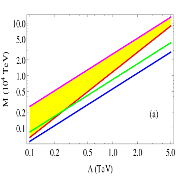
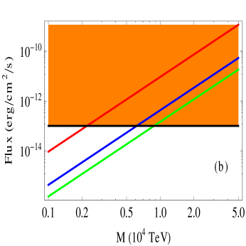
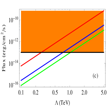
Figure 1: Constraints on the parameters $M,\Lambda$ due to the observations made by Chandra telescope. In plot (a) anything below the thick red line is excluded in the plane $M-\Lambda$. The blue and magenta lines are contour lines where the neutrino mass scales are 1 eV and 0.01 eV, respectively. Points along the green line in this plot fits the 100$\%$ relic density of the present universe. The shaded yellow region is allowed by both the X-ray flux and the neutrino mass scale restrictions. In plots (b) and (c) X-ray flux from various clusters are plotted as a function of $M$ and $\Lambda$. $\Omega_{s}h^{2}$ = 0.1 is taken in both these plots. The red, blue and green lines in these plots are for the X-ray flux due to sterile neutrinos coming from the clusters Virgo center, NGC 3198, NGC 4123, respectively The shaded orange region in these plots is excluded.

We have used $M^{\rm fov}_{\rm DM}=10^{13}M_{\odot}$ and $D_{L}=$ 20.7 Mpc [10] in eq. (12) and demanded that the flux should be less than the detectable limit $10^{-13}$ erg cm^-2 s^-1. The thick red line in this figure represents this flux restriction. Anything below this line can be considered to be ruled out. The blue and magenta lines in this plot represent contour lines of constant neutrino mass scale of 1 eV and 0.01 eV, respectively. The first relation of eq. (7) gives neutrino mass scale as a function of $\Lambda$ and $M$. Although the neutrino mass scale is around 0.1 eV, in Fig. 1(a) we have allowed flexibility in the neutrino mass scale to be between 1 eV and 0.01 eV. The solar neutrino mass scale is $\approx$ 0.009 eV, which is a few factor less than the atmospheric scale of $\approx$ 0.05 eV. It is stated before that the neutrino mass scale of eq. (7) gives a rough estimation. As a consequence of this it may not be realistic to fit the neutrino oscillation data for a neutrino mass scale less than about 0.01 eV. Hence, the yellow shaded region in Fig. 1(a) can be taken to be as allowed region by the X-ray flux restriction and the neutrino mass of this model. However, in the flux restriction we do not demand that the sterile neutrinos to be exactly as warm dark matter particles, but we only require them to decay radiatively to a photon. Stringent bounds can be obtained on these parameters if we demand the sterile neutrino to fit 100$\%$ of the current relic density of the universe. For relic abundance we have taken $\Omega_{s}h^{2}=$ 0.1 which falls within the experimental limits of it as observed by the Wilkinson Microwave Anisotropy Probe (WMAP) [19]. The thick green line in Fig. 1(a) represents a contour line in the parameters where $\Omega_{s}h^{2}=$ 0.1. We have given the individual constraints on the $M$ and $\Lambda$ in Figs. 1(b) and 1(c), which arise due to both the X-ray flux restriction and also by the demand of 100$\%$ relic abundance from the sterile neutrino. By putting $\Omega_{s}h^{2}=$ 0.1, we have plotted flux versus $M$ in Fig. 1(b) and flux versus $\Lambda$ in Fig. 1(c), using eqs. (12) and (13). In both these plots we have also given restrictions coming from clusters NGC 3198 and NGC 4123, in order to compare with the results obtained from Virgo cluster. The red line in both these plots is for Virgo cluster, the blue line is for NGC 3198 and the green line is for NGC 4123, respectively. The values of $(M^{\rm fov}_{\rm DM},D_{L})$ for NGC 3198 and NGC 4123 are (3.62$\times 10^{11}M_{\odot}$, 18.34 Mpc) and (1.85$\times 10^{11}M_{\odot}$, 22.4 Mpc), respectively [10]. The orange shaded region in both Figs. 1(b) and 1(c) is the disallowed region. We can see that Virgo cluster put upper bound on the $M$ to be less than about 0.2$\times 10^{4}$ TeV and the corresponding bound on the scale $\Lambda$ is less than 0.3 TeV. The bounds from the clusters of NGC’s on $M$ and $\Lambda$ are reasonable but they are less stringent than that due to the Virgo cluster.

We remind here that we have neglected the ${\cal O}(1)$ constants in eq. (7). These ${\cal O}(1)$ constants will change the flux and relic density relations, eqs. (12) and (13), by some factors. If the resultant factor in the flux relation of eq. (12) is less than one, we expect the red line of Fig. 1(a) to shift little bit down, and hence the constraint due to flux restriction will be weakened. The opposite effect happens if this factor is greater than one. Similar behavior can be expected for the relic density constraint of eq. (13) due to these factors. Although we do not expect the constraints to change significantly away from what we have obtained in Fig. 1, we leave this for a detailed study later. Another point to note here is that in Fig. 1(a), we have plotted from $\Lambda$ = 0.1 TeV, where the corresponding allowed value of $M$ by neutrino mass and flux restriction would be $\sim 10^{3}$ TeV. For this $\Lambda$ and $M$ values we not only get 0.1 eV neutrino masses but also viable keV sterile neutrinos, as explained below eq. (7). Although big-bang nucleosynthesis put a lower bound on $\Lambda$ to be $\sim$ 1 GeV [7], for such a low value of $\Lambda$ it is not possible to get $m_{\nu}\sim$ 0.1 eV and $m_{s}\sim$ keV by using eq. (7).

After giving constraints on the composite Dirac neutrino model due to the observations made by Chandra telescope, we now give constraints on this model from different data analysis. In [12], data collected by XMM-Newton on Coma and Virgo clusters have been analyzed. Here, it has been pointed that the background due to continuum X-rays from intra-cluster gas can be reduced compared to the signal if the flux at the periphery is collected. Accordingly, we can analyze flux from the center and periphery of both Coma and Virgo clusters. From this analysis we can see that the data from Coma periphery put stringent limits among all these observations. The method employed in getting the constraints is explained as follows. The experiment XMM-Newton has collected data in the energy region of 0.5 to 8.5 keV. This region has been divided into bins of size 0.2 keV. By demanding the X-ray flux from dark matter in the center of each of the energy bin to be less than the detected flux in that bin, an exclusion plot in the plane $\sin^{2}2\theta-m_{s}$ can be obtained. Below we give the formulas for the flux with projected radius $r$ from Coma and Virgo clusters, respectively [12]:

$$F_{\rm Coma} \approx 6.7\times 10^{-8}\theta^{2}\left(\frac{m_{s}}{1{\rm keV}}\right)^{5}g(r)~{}{\rm erg~{}cm^{-2}~{}s^{-1}},$$

$$F_{\rm Virgo} \approx 7.7\times 10^{-9}\theta^{2}\left(\frac{m_{s}}{1{\rm keV}}\right)^{5}g(r)~{}{\rm erg~{}cm^{-2}~{}s^{-1}}.$$ (14)

Here, $g(r)$ is a geometric factor with projected radius $r$. For Coma center and periphery its values are 0.82 and 0.18 respectively, whereas, for Virgo center (M87) the geometric factor is 6.8 [12]. Although the actual exclusion line in the plane $\sin^{2}2\theta-m_{s}$ would be obtained by demanding the flux values from above equations in a energy bin to be less than the measured flux in that energy bin, a rough understanding on these constraints can be understood by plotting the contour lines in the plane $\sin^{2}2\theta-m_{s}$ for a constant flux at 0.5 keV and 8.5 keV. Imagine we are doing analysis on the data from Coma periphery. By putting the geometric factor for this source in $F_{\rm Coma}$, we plot contour lines in $\sin^{2}2\theta-m_{s}$ for the relations: $F_{\rm Coma}=F_{0.5keV}$ and $F_{\rm Coma}=F_{8.5keV}$, where $F_{0.5keV}$ and $F_{8.5keV}$ are the observed flux values in the experiment at the energy bins containing 0.5 keV and 8.5 keV, respectively. These two contour lines give a rough estimation on the exclusion area in the plane $\sin^{2}2\theta-m_{s}$. But the actual exclusion line from the full analysis lie in between these two extreme contour lines. We demonstrate this when we present our results on the composite Dirac neutrinos below. However, the exclusion in the parameters of $(\sin^{2}2\theta,m_{s})$ from the analysis done on the coma periphery by the XMM-Newton telescope can be parameterized as [12]

$$\sin^{2}(2\theta)\leq 3.76\times 10^{-4}\left(\frac{m_{s}}{\rm 1keV}\right)^{-5.63}$$ (15)

To translate the above restrictions from the data by XMM-Newton into the composite Dirac neutrino model, we include a half-factor in the flux relations since in the analysis described above Majorana neutrinos have been assumed. Using eq. (7), the flux relations for the Dirac neutrinos turn out to be:

$$F_{\rm Coma} \approx 3.35\times 10^{-11}\left(\frac{v}{\rm 1TeV}\right)^{2}\left(\frac{\Lambda}{\rm 1TeV}\right)^{15}\left(\frac{10^{4}~{}\rm TeV}{M}\right)^{12}g(r)~{}{\rm erg~{}cm^{-2}~{}s^{-1}},$$

$$F_{\rm Virgo} \approx 3.85\times 10^{-12}\left(\frac{v}{\rm 1TeV}\right)^{2}\left(\frac{\Lambda}{\rm 1TeV}\right)^{15}\left(\frac{10^{4}~{}\rm TeV}{M}\right)^{12}g(r)~{}{\rm erg~{}cm^{-2}~{}s^{-1}}.$$ (16)

The relation of eq. (15) will translate in our case as

$$\left(\frac{M}{10^{4}~{}\rm TeV}\right)^{13.26}\geq\frac{2}{3.76}10^{1.63}\left(\frac{v}{\rm 1TeV}\right)^{2}\left(\frac{\Lambda}{\rm 1TeV}\right)^{16.89}.$$ (17)

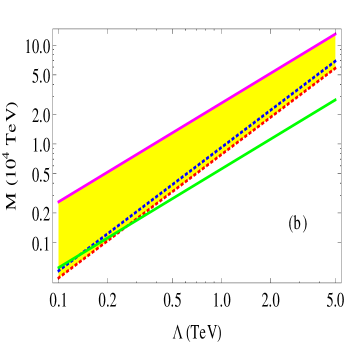
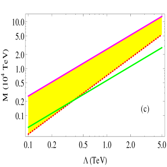
Figure 2: Constraints in the plane $M-\Lambda$ from the data collected by XMM-Newton telescope. Anything below the red dotted line in these figures are ruled out. The green and magenta lines are contour lines where the neutrino mass scale are 1 eV and 0.01 eV respectively. The yellow shaded region is allowed by both the X-ray flux and neutrino mass scale restrictions. Constraints in the plots (a), (b) and (c) are due to the data from Coma periphery, Coma center and Virgo center, respectively.

The constraints due to Coma periphery are given in Fig. 2(a). The red and blue dotted lines in this plot represents the constant contour lines for $F_{\rm Coma}=F_{0.5\rm keV}$ and $F_{\rm Coma}=F_{8.5\rm keV}$, respectively. The actual constraint due to the full analysis of eq. (17) is given in thick dark line which almost touches the constant contour lines at both the extreme ends. The values for the flux from Coma periphery are taken as: $F_{0.5\rm keV}=1.1\times 10^{-12}~{}{\rm erg~{}cm^{-2}~{}s^{-1}}$, $F_{8.5\rm keV}=9.0\times 10^{-14}~{}{\rm erg~{}cm^{-2}~{}s^{-1}}$ [12]. Anything below the dark line is disallowed. But it can be noticed that the red dotted line in this plot gives a conservative bound and, whereas the blue dotted line gives a slightly stringent overestimated bound compared to the dark line. Hence the constant flux contour lines at the extreme energy bins give a rough estimation of the constraints. In Fig. 2(a) we have also given the contour lines of constant neutrino mass scale. The green and magenta lines in this plot represent a constant neutrino mass scale of 1 eV and 0.01 eV respectively. As explained previously that the neutrino mass scale below 0.01 eV may not fit the neutrino oscillation data, and hence the yellow shaded region between the dark line and the magenta line is considered to be allowed region in the plane $M-\Lambda$. In Fig. 2(b) constraints due to the Coma center are given in the plane $M-\Lambda$. We have given the constant flux contour lines of $F_{\rm Coma}=F_{0.5\rm keV}=1.6\times 10^{-11}~{}{\rm erg~{}cm^{-2}~{}s^{-1}}$ and $F_{\rm Coma}=F_{8.5\rm keV}=2.2\times 10^{-12}~{}{\rm erg~{}cm^{-2}~{}s^{-1}}$ [12], which are indicated in red and blue dotted lines, respectively. Anything below the red dotted line can be considered to be excluded, but the blue dotted line gives a somewhat overestimated stringent bound. The actual constraint from the full analysis would lie somewhere between the red and blue dotted lines, similar to the case of Coma periphery which is explained above. The green and magenta lines in this plot give constant neutrino mass scale of 1 eV and 0.01 eV respectively. The yellow shaded region is allowed from the X-ray flux and the neutrino mass constraints. In Fig. 2(c) we have given constraints due to Virgo center as observed by the XMM-Newton telescope. In this plot we have a constant contour line of $F_{\rm Virgo}=F_{1\rm keV}=4.8\times 10^{-11}~{}{\rm erg~{}cm^{-2}~{}s^{-1}}$ [12], which is shown in the red dotted line. Like for the previous plots anything below this line can be considered to be ruled out, and also the yellow shaded region is allowed from the X-ray flux and the neutrino mass scale constraints.

Comparing the constraints from various sources in Fig. 2, Coma periphery put stringent limits due to the fact that the observed flux from it is at least an order less than that due to the other sources. In any of the plots of Fig. 2 we have not applied the restriction that the sterile neutrino should fit the 100$\%$ of the relic density of the universe. However, if applied, like we have done in Fig. 1, we may expect similarly stringent limits on both the scales $M$ and $\Lambda$.

4 Conclusions

In the era of the Large Hadron Collider, where we are in now, it is important to analyze the new physics models and if possible put constraints in a model. However, apart from collider data, astrophysical experiments also play a role in probing the new physics models which have relation to cosmology. We have analyzed one of those models where Dirac neutrino masses can only appear as a result of confinement of a UV preonic theory at a high scale $M$ into some hidden sector and standard model fields, and the hidden sector confines into right-handed neutrinos at a lower scale $\Lambda\ll M$ [5]. Both the scales $M$ and $\Lambda$ determine the masses of the active and sterile neutrinos, and also the mixing angle between them. In the case of secondary mass generation for the sterile neutrinos, and for $\Lambda\sim$ TeV and $M\sim 10^{4}$ TeV, we get keV mass sterile neutrinos with a mixing angle of $\sim 10^{-5}$ with the active neutrinos, apart from getting the correct neutrino mass scale of 0.1 eV. The keV mass sterile neutrinos form viable warm dark matter candidates. One of the channels to probe the sterile neutrino is its decay to an X-ray photon and an active neutrino, which has been looked in astrophysical experiments like Chandra and XMM-Newton. The mass scale and the mixing angle for the sterile neutrino in this particular model falls in the right ball park region analyzed in these experiments. Hence, we have studied constraints on the model parameters $\Lambda$ and $M$ due to the negative search of these particles in the astrophysical experiments. A previous study on this kind of model has put a lower bound of $\sim$ 1 GeV on the parameter $\Lambda$ from the big-bang nucleosynthesis [7]. Whereas, in this work we have shown that from the X-ray analysis and also if the sterile neutrino make up 100$\%$ of the dark matter, we can get upper bounds on both of the parameters $\Lambda$ and $M$.

More specifically, from the analysis of the data collected by Chandra telescope on Virgo cluster we have obtained an upper bound on the scale $M$ to be about 2$\times 10^{3}$ TeV if it fits the 100$\%$ of the current relic abundance of the universe. Under the same assumption the corresponding upper bound on the scale $\Lambda$ is $\sim$ 300 GeV. From the data collected by the XMM-Newton telescope on the periphery of the Coma cluster, we got stringent limits in the plane of $M$ and $\Lambda$. However, in this analysis we have not applied the condition that the sterile neutrino should fit the 100$\%$ of the relic abundance of the universe, but, if applied we may get similar constraints as mentioned above. In both the analysis that we have mentioned above, we have also given region of parametric space in the plane $M-\Lambda$ allowed by both the neutrino mass scale and the X-ray flux restrictions.

References

- [1] R. Davis, Phys. Rev. Lett. 12 303 (1964); R. Davis et al., Phys. Rev. Lett. 20, 1205 (1968); Y. Fukuda et al. (Kamiokande Collaboration), Phys. Rev. Lett. 77, 1683 (1996); W. Hampel et al. (Gallex Collaboration), Phys. Lett. B 447, 127 (1999); J.N. Abdurashitov et al. (SAGE Collaboration), Phys. Rev. C 60, 055801 (1999); Q.R. Ahmad et al. (SNO Collaboration), Phys. Rev. Lett. 87, 071301 (2001); K. Eguchi et al. (KamLAND Collaboration), Phys. Rev. Lett. 90, 021802 (2003); J. Hosaka et al. (Super-Kamkiokande Collaboration), Phys. Rev. D 73, 112001 (2006).
- [2] Y. Fukuda et al. (Super-Kamkiokande Collaboration), Phys. Rev. Lett. 81, 1562 (1998); M. Ambrosio et al. (MACRO Collaboration), Phys. Lett. B 434, 451 (1998).
- [3] P. Minkowski, Phys. Lett. B 67, 421 (1977); T. Yanagida, in Proceedings of the workshop on unified theory and baryon number in the universe, KEK, March 1979, eds. O. Sawada and A. Sugamoto; M. Gell-Mann, P. Ramond and R. Slansky, in Supergravity, Stonybrook, 1979, eds. D. Freedman and P. van Nieuwenhuizen; S.L. Glashow, The future of elementary particle physics, in Proceedings of the 1979 Cargèse Summer Institute on Quarks and Leptons (M. Lévy et al. eds.), Plenum Press, New York, 1980, pp. 687; R.N. Mohapatra and G. Senjanović, Phys. Rev. Lett. 44, 912 (1980); J. Schechter and J.W.F. Valle, Phys. Rev. D 22, 2227 (1980); G.B. Gelmini and M. Roncadelli, Phys. Lett. B 99, 411 (1981).
- [4] L.M. Krauss and F. Wilczek, Phys. Rev. Lett. 62, 1221 (1989); P. Langacker, Phys. Rev. D 58, 093017 (1998); K.R. Dienes, E. Dudas and T. Gherghetta, Nucl. Phys. B 557, 25 (1999); Y. Grossman and M. Neubert, Phys. Lett. B 474, 361 (2000); I. Gogoladze and A. Perez-Lorenzana, Phys. Rev. D 65, 095011 (2002); N. Arkani-Hamed, S. Dimopoulos, G.R. Dvali and J. March-Russell, Phys. Rev. D 65, 024032 (2002); P.Q. Hung, Phys. Rev. D 67, 095011 (2003); T. Gherghetta, Phys. Rev. Lett. 92, 161601 (2004); H. Davoudiasl, R. Kitano, G.D. Kribs and H. Murayama, Phys. Rev. D 71, 113004 (2005); S. Abel, A. Dedes and K. Tamvakis, Phys. Rev. D 71, 033003 (2005); M.-C. Chen, A. de Gouvea and B.A. Dobrescu, Phys. Rev. D 75, 055009 (2007); D.A. Demir, L.L. Everett and P. Langacker, Phys. Rev. Lett. 100, 091804 (2008); G. von Gersdorff and M. Quiros, Phys. Lett. B 678, 317 (2009); G. Marshall, M. McCaskey and M. Sher, Phys. Rev. D 81, 053006 (2010).
- [5] Y. Grossman and D.J. Robinson, JHEP 1101, 132 (2011).
- [6] N. Arkani-Hamed and Y. Grossman, Phys. Lett. B 459, 179 (1999); Y. Grossman and Y. Tsai, JHEP 0812, 016 (2008).
- [7] T. Okui, JHEP 0509, 017 (2005).
- [8] S. Dodelson and L.M. Widrow, Phys. Rev. Lett. 72, 17 (1994); T. Asaka, S. Blanchet and M. Shaposhnikov, Phys. Lett. B 631, 151 (2005); T. Asaka, M. Shaposhnikov and A. Kusenko, Phys. Lett. B 638, 401 (2006); A. Kusenko, Phys. Rept. 481, 1 (2009).
- [9] C.R. Watson, J.F. Beacom, H. Yuksel and T.P. Walker, Phys. Rev. D 74, 033009 (2006); S. Riemer-Sorensen, K. Pedersen, S.H. Hansen and H. Dahle, Phys. Rev. D 76, 043524 (2007); D. Cumberbatch and J. Silk, AIP Conf. Proc. 957, 375 (2007) [arXiv:0709.0279 [astro-ph]]; H. Yuksel, J.F. Beacom and C.R. Watson, Phys. Rev. Lett. 101, 121301 (2008).
- [10] K. Abazajian, G.M. Fuller and W.H. Tucker, Astrophys. J. 562, 593 (2001).
- [11] M. Mapelli and A. Ferrara, Mon. Not. Roy. Astron. Soc. 364, 2 (2005); A. Boyarsky, A. Neronov, O. Ruchayskiy and M. Shaposhnikov, Mon. Not. Roy. Astron. Soc. 370, 213 (2006).
- [12] A. Boyarsky, A. Neronov, O. Ruchayskiy and M. Shaposhnikov, Phys. Rev. D 74, 103506 (2006).
- [13] S.H. Hansen, J. Lesgourgues, S. Pastor and J. Silk, Mon. Not. Roy. Astron. Soc. 333, 544 (2002); M. Viel, J. Lesgourgues, M.G. Haehnelt, S. Matarrese and A. Riotto, Phys. Rev. D 71, 063534 (2005).
- [14] K.L. McDonald, Phys. Lett. B 696, 266 (2011).
- [15] S. Dimopoulos, S. Raby and L. Susskind, Nucl. Phys. B 173, 208 (1980); R.D. Peccei, in Gauge Theories of the Eighties, Vol. 181 (Springer Berlin, 1983) p. 355.
- [16] M. Loewenstein and A. Kusenko, Astrophys. J. 714, 652 (2010).
- [17] P.B. Pal and L. Wolfenstein, Phys. Rev. D 25, 766 (1982).
- [18] K. Abazajian, G.M. Fuller and M. Patel, Phys. Rev. D 64, 023501 (2001).
- [19] E. Komatsu et al. (WMAP Collaboration), Astrophys. J. Suppl. 192, 18 (2011).