Cosmic Ray Electron and Positron Excesses
from a Fourth Generation Heavy Majorana Neutrino

Abstract

Unexpected features in the energy spectra of cosmic rays electrons and positrons have been recently observed by PAMELA and Fermi-LAT satellite experiments, opening to the exciting possibility of an indirect manifestation of new physics. A TeV-scale fourth lepton family is a natural extension of the Standard Model leptonic sector (also linked to the hierarchy problem in Minimal Walking Technicolor models). The heavy Majorana neutrino of this setup mixes with Standard Model charged leptons through a weak charged current interaction. Here, we first study analytically the energy spectrum of the electrons and positrons originated in the heavy Majorana neutrino decay modes, also including polarization effects. We then compare the prediction of this model with the experimental data, exploiting both the standard direct method and our recently proposed Sum Rules method. We find that the decay modes involving the tau and/or the muon charged leptons as primary decay products fit well the PAMELA and Fermi-LAT lepton excesses while there is tension with respect to the antiproton to proton fraction constrained by PAMELA.
Preprint: CP³-Origins-2011-15
Preprint: DIAS-2011-01

I Introduction

A hardening in the electron and positron fluxes has been observed in Cosmic Rays (CRs) at energies between $10$ GeV and $1$ TeV. More precisely, PAMELA Adriani:2008zr measured a rise in the positron fraction above $10$ GeV. Fermi-LAT Abdo:2009zk measured the sum of the positron and electron fluxes, detecting a feature with spectral index of about -3 above $100$ GeV, followed by a decrease at $500$ GeV. The latter results strengthened previous hints by ATIC :2008zzr and PPB-BETS Torii:2008xu balloon experiments and by the ground-based telescope HESS Aharonian:2008aa .

When compared with the predictions of current astrophysical models, the results of PAMELA and Fermi-LAT independently suggest the presence of an excess of electrons and/or positrons. The origin of these excesses is unknown and many explanations have been put forward: from misunderstood astrophysical effects to new physics indirect effects. Notice that the lack of any excess in antiproton CRs found by PAMELA Adriani:2010rc is a crucial element in understanding the origin the electron and positron excesses. Interpreting these excesses as signatures of a dark matter component, generically an annihilating or decaying WIMP, is for sure exciting; see e.g. Fan:2010yq for a review.

While the interpretation in terms of dark matter annihilations often leads to an unobserved excess of gamma and radio photons, the interpretation in terms of dark matter decays is compatible with photon observations Nardi:2008ix ; Ibarra:2009nw , even though some channels now start to show some tension Cirelli:2009dv ; Meade:2009iu ; Papucci:2009gd ; Hutsi:2010ai . A discrimination strategy was proposed in Boehm:2010qt ; PalomaresRuiz:2010uu .

In this work, we want to investigate a simple extension of the Standard Model (SM): a heavy Majorana neutrino $N$ which couples to SM particles only via charged current interaction:

$${\cal L}^{CC}_{\ell N}=-i\frac{g}{\sqrt{2}}~{}C_{\ell}~{}W_{\mu}^{-}\bar{\ell}\gamma^{\mu}P_{L}N+h.c.$$ (1)

where $C_{\ell}$, with $\ell=e,\mu,\tau$, is a numerical factor parametrizing the strength of the mixing between the heavy neutrino $N$ and the SM charged lepton $\ell$ and $P_{L}$ is the L-chirality projector. The interaction above naturally arises extending the SM leptonic sector by introducing a fourth lepton family, as happens e.g. in Minimal Walking Technicolor models Sannino:2004qp ; Dietrich:2005jn ; Foadi:2007ue ; Frandsen:2009fs ; Antipin:2009ks ; Andersen:2011yj .

We are interested in a nearly stable and TeV-scale heavy neutrino, which could constitute a fraction of the dark matter density, $x_{N}=\rho_{N}/\rho_{DM}$. Via its semileptonic decays $N\rightarrow\ell^{\pm}W^{\mp}$ – whose branching ratio (BR) into the specific flavor $\ell$ is proportional to $C_{\ell}^{2}$ – the heavy Majorana neutrino could also be a source of electron and positron CRs. Our goal is to study whether the electron and positron excesses observed by PAMELA and Fermi-LAT can be attributed to such decaying heavy Majorana neutrino. Notice that in our model the fluxes of electrons and positrons coming from the $N$ decay chains are equal.

We focus on a very specific model: we are thus able to discard the model if it turns out not to fit the data, or to strongly constrain its parameter space. Instead of using numerical codes Ibarra:2008qg ; Ibarra:2008jk ; Ibarra:2009dr ; Nardi:2008ix ; Meade:2009iu ; Cirelli:2010xx , for each lepton flavor $\ell$ here we calculate analytically the energy spectra of the electrons and positrons produced in $N\rightarrow\ell W$ and the subsequent $\ell$ and $W$ decay chains, including polarization effects. This allows to have a deeper understanding of the physical results and, as we are going to discuss, to find features that are not properly accounted for in some numerical codes. We then consider the propagation of electrons and positrons according to the most popular models and compare our predictions with the experimental results of PAMELA and Fermi-LAT, exploiting both the more straightforward Sum Rules (SR) method proposed in ref.Frandsen:2010mr and the longer direct comparison method.

Considering in turn each channel $N\rightarrow\ell W$ (with $\ell=e,\mu,\tau$) and its subsequent decays, we find that: the decays into $\tau W$ fit the experimental data extremely well for $M_{N}\approx 3$ TeV and $x_{N}^{1/2}C_{\tau}\approx 10^{-27}$; a good fit is obtained for the decays into $\mu W$ for the same model parameters; while it is impossible to reproduce the data if $N$ decays mostly into $eW$.

As for the CR antiproton contribution from the heavy Majorana neutrino decays, in ref.Ibarra:2009dr it was estimated to be compatible with the PAMELA experimental data. In ref. Nardi:2008ix there was some tension with the data, but a fit to the ATIC data were used there. We have redone the analysis for the antiproton flux as well as the antiproton to proton fraction for the processes relevant here and compared to CAPRICE Boezio:2001ac and PAMELA Adriani:2010rc data. We find that it is possible to accommodate the CAPRICE data while we observe a tension with the PAMELA data.

We conclude that a $3$-TeV fourth family Majorana neutrino with dominant BR into $\tau W$ and/or $\mu W$ with coupling $x_{N}^{1/2}C_{\tau/\mu}\approx 10^{-27}$ represents a plausible and even quite conservative explanation of the electron and positron CRs excesses.

Our findings confirm previous numerical studies for the $e$ and $\mu$ channel, but disagree for the $\tau$ channel, which was considered to be disfavored Ibarra:2009dr or to provide a worse fit to the data as compared to the $\mu$ channel Meade:2009iu . These analysis were based on the Monte Carlo simulation program PYTHIA which (as well as HERWIG) treats leptons and vector bosons as unpolarized. To understand the origin of this discrepancy, we carried out our analysis also neglecting polarization effects. We find that, although going in the right direction, polarization effects cannot alone explain the discrepancy between our analytically-based results and the numerically-based results of previous analyses. A comparison with ref. Nardi:2008ix is not strictly possible, since polarization effects were neglected and especially the ATIC data :2008zzr were used for the fits, not the subsequent ones by Fermi-LAT Abdo:2009zk . On the other hand, in the more recent analysis of ref.Cirelli:2010xx including polarization and even electroweak emission Ciafaloni:2010ti , the semileptonic decay channels were not considered.

The paper is organized as follows. In section II the model setup is introduced. In section III the analytical calculation of the energy spectrum of electrons and positrons from $N$ decays is carried out, studying separately each of the three semileptonic channels. Section IV is devoted to the comparison of the model prediction with the experimental data, bot with the SR and direct comparison methods. Section V presents the estimate for the antiproton flux and antiproton-proton ratio. We draw our conclusions in section VI.

II The fourth lepton family setup

In the SM, the three lepton families, $\ell=e,\mu,\tau$, belong to the following representations of the gauge group $SU(3)_{c}\times SU(2)_{L}\times U(1)_{Y}$:

$$L_{\ell}=({\nu_{\ell}}_{L}~{}~{}\ell_{L})^{T}\sim(1,2,-1/2)~{}~{}~{}~{}~{},~{}~{}~{}~{}~{}\ell_{R}\sim(1,1,-1)~{}~{}~{}~{}~{}.$$ (2)

where the chirality projectors $P_{L}=(1-\gamma_{5})/2$ and $P_{R}=(1+\gamma_{5})/2$ have been introduced. It has been observed experimentally that at least two of the SM neutrinos have a small mass, not larger than the eV-scale pdg2010 . In the following, we account for light neutrino masses and mixings via an effective Majorana mass term, i.e. by adding to the SM Lagrangian a dimension-5 non-renormalizable operator (which could arise for instance through a seesaw mechanism).

Our aim here is to investigate the CR positron and electron fluxes originated via the decay of a possible TeV-scale fourth lepton family, for which we introduce the $\zeta$-flavor. This additional family is composed by a lepton doublet, a charged lepton singlet and a gauge singlet:

$$L_{\zeta}=({\nu_{\zeta}}_{L}~{}~{}\zeta_{L})^{T}\sim(1,2,-1/2)~{}~{}~{}~{},~{}~{}~{}~{}~{}{\zeta}_{R}\sim(1,1,-1)~{}~{}~{},~{}~{}~{}~{}~{}{\nu_{\zeta}}_{R}\sim(1,1,0)~{}~{}.$$ (3)

We keep our scenario as general as possible, but we stress that it would arise naturally in Minimal Walking Technicolor models Sannino:2004qp , with interesting collider signatures Frandsen:2009fs - see also Antipin:2009ks and, for a complete review, ref.Andersen:2011yj .

The $\zeta$-charged lepton, $\zeta={\zeta}_{L}+{\zeta}_{R}$, has a Dirac mass term like the other three charged leptons of the SM, but large enough to avoid conflict with the experimental limits. We work in the basis in which the $4\times 4$ charged lepton mass matrix is diagonal. The mass eigenstates of the two electrically neutral Weyl fermions instead correspond to two Majorana neutrinos, $N_{1,2}$, for which we are free to choose the ordering $M_{N_{1}}\leq M_{N_{2}}$. In such a framework, assuming the $\zeta$ lepton to be heavy enough with respect to $N_{1}$, it turns out that the latter is stable and can constitute - at least part of - the dark matter in our galaxy.

We consider the possibility that the new heavy leptons mix with the SM leptons. For clarity of presentation, we assume that the heavy neutrinos mix only with one SM neutrino of flavor $\ell$ ($\ell=e,\mu,\tau$). This is not a restrictive assumption: as demonstrated in appendix A, the expressions that we are going to derive apply also to the case in which the heavy neutrinos mix simultaneously with all three light lepton families. The entries of the mass matrix are:

$$-{\cal L}_{mass}=\frac{1}{2}(\begin{array}[]{ccc}\overline{(\nu_{\ell L})^{c}}&\overline{(\nu_{\zeta L})^{c}}&\overline{\nu_{\zeta R}}\end{array})\left(\begin{array}[]{ccc}{\cal O}(eV)&{\cal O}(eV)&m_{\ell}\cr{\cal O}(eV)&{\cal O}(eV)&m_{D}\cr m_{\ell}&m_{D}&m_{R}\end{array}\right)\left(\begin{array}[]{c}\nu_{\ell L}\cr\nu_{\zeta L}\cr(\nu_{\zeta R})^{c}\end{array}\right)+h.c.~{}~{}.$$ (4)

The measured values of the light neutrino masses suggest that the entries of the upper 2$\times$2 block have to be of ${\cal O}(eV)$. The mass scale of $m_{R}$ could be as large as the cutoff of the theory, since it is not protected by any symmetry (we allow violation of the lepton flavour number $L_{\zeta}$ by 2 units). The elements $m_{\ell}$ and $m_{D}$ are expected to be at most of the order of the electroweak scale. Given such a hierarchical structure and up to small corrections of ${\cal O}(eV/M_{N_{1},N_{2}})\lesssim 10^{-11}$, one obtains the following form for the unitary matrix which diagonalises eq.(4):

$$\left(\begin{array}[]{c}\nu_{\ell L}\cr\nu_{\zeta L}\cr(\nu_{\zeta R})^{c}\end{array}\right)=V\left(\begin{array}[]{c}N_{\ell L}\cr N_{1L}\cr N_{2L}\end{array}\right)~{}~{},~{}~{}V=\left(\begin{array}[]{ccc}\cos\theta_{\ell}&i\cos\theta\sin\theta_{\ell}&\sin\theta\sin\theta_{\ell}\cr-\sin\theta_{\ell}&i\cos\theta\cos\theta_{\ell}&\sin\theta\cos\theta_{\ell}\cr 0&-i\sin\theta&\cos\theta\end{array}\right).$$ (5)

$N_{\ell,1,2}$ are the new Majorana mass eigenstates (actually $N_{\ell}$ is a flavor eigenstate when including all three SM leptons, as discussed in the appendix) and

$$\tan\theta_{\ell}=\frac{m_{\ell}}{m_{D}}~{}~{}~{},~{}~{}~{}~{}~{}\tan 2\theta=2~{}\frac{\sqrt{m_{D}^{2}+m_{\ell}^{2}}}{m_{R}}~{}~{}~{}.$$ (6)

The light neutrino $N_{\ell}$ has a mass of ${\cal O}(eV)$. Up to corrections of ${\cal O}(eV)$, the heavy neutrinos $N_{1,2}$ have positive masses given by:

$$M_{N_{1}}=\frac{m_{R}}{2}\left(\sqrt{1+4\frac{m_{D}^{2}+m_{\ell}^{2}}{m_{R}^{2}}}-1\right)~{}~{},~{}~{}~{}~{}M_{N_{2}}=\frac{m_{R}}{2}\left(\sqrt{1+4\frac{m_{D}^{2}+m_{\ell}^{2}}{m_{R}^{2}}}+1\right)~{}.$$ (7)

The smaller is $m_{R}$ (namely the more $\theta$ approaches $\pi/4$), the more the neutrinos $N_{1}$ and $N_{2}$ become the two Weyl components of a Dirac state. Notice that the mixing between the heavy neutrino states $N_{1,2}$ is controlled by the mixing angle $\theta_{\ell}$, which is constrained experimentally to be small (more on this later).

The neutral current interactions of the neutrinos are

$${\cal L}^{NC}_{N}=\frac{g}{4\cos\theta_{w}}Z_{\mu}(\bar{N}_{\ell}\gamma^{\mu}\gamma_{5}N_{\ell}+\cos^{2}\theta~{}\bar{N}_{1}\gamma^{\mu}\gamma_{5}N_{1}+\sin^{2}\theta~{}\bar{N}_{2}\gamma^{\mu}\gamma_{5}N_{2}-i\sin(2\theta)~{}\bar{N}_{2}\gamma^{\mu}N_{1})\ ,$$ (8)

while their charged current interactions with the light and heavy charged leptons are respectively

$${\cal L}^{CC}_{\zeta N}=-\frac{g}{\sqrt{2}}W_{\mu}^{-}\bar{\zeta}_{L}\gamma^{\mu}(-\sin\theta_{\ell}N_{\ell L}+i\cos\theta\cos\theta_{\ell}N_{1L}+\sin\theta\cos\theta_{\ell}N_{2L})+h.c.$$ (9)

and

$${\cal L}^{CC}_{\ell N}=-\frac{g}{\sqrt{2}}W_{\mu}^{-}\bar{\ell}_{L}\gamma^{\mu}(\cos\theta_{\ell}N_{\ell L}+i\cos\theta\sin\theta_{\ell}N_{1L}+\sin\theta\sin\theta_{\ell}N_{2L})+h.c.~{}~{}.$$ (10)

Notice that the neutrino neutral current remains flavor diagonal at tree-level (the neutral current is not flavor diagonal in models with TeV scale right handed neutrinos involved in the see-saw mechanism for the light SM neutrino masses, see e.g. del Aguila:2007em ), hence the heavy neutrinos couple to the SM ones only through the charged current interactions at this order. This is a distinctive feature of our fourth lepton family.

Indeed, also the Yukawa interactions do not mix the heavy Majorana neutrinos with the SM one:

$${\cal L}^{H}_{N}=-\frac{g~{}(\cos\theta_{\ell}m_{D}+\sin\theta_{\ell}m_{\ell})}{2M_{W}}\left(\frac{\sin(2\theta)}{2}({\bar{N}_{1}}N_{1}+{\bar{N}_{2}}N_{2})-i\cos(2\theta){\bar{N}_{1}}\gamma_{5}N_{2}\right)H~{}.$$ (11)

In this work we are then concerned with a heavy Majorana neutrino $N_{1}$, which only couples to the SM charged leptons, and with a small mixing angle. If such mixing is small enough, $N_{1}$ can be considered as nearly stable on cosmological time scales. We assume $M_{\zeta}>M_{1}+M_{W}$, so that the charged lepton $\zeta$ already disappeared as a dark matter candidate because of its decays into $WN_{1}$.

As for the possible hierarchies between the heavy neutrinos, two main situations arise: if $M_{N_{2}}>M_{N_{1}}+M_{Z}$, also $N_{2}$ already disappeared; if $M_{N_{2}}<M_{N_{1}}+M_{Z}$, $N_{2}$ is nearly stable like $N_{1}$ (in the limit of degenerate masses they form a Dirac neutrino). From now on, we consider the first scenario.

II.1 Laboratory constraints

From collider experiments there are both direct and indirect constraints on heavy leptons. We refer to Frandsen:2009fs for an updated analysis (together with some useful references) and here we just summarize the results relevant for the present analysis.

As stressed, we are concerned with a heavy neutrino $N_{1}$ which is nearly stable on cosmological time scales. For this setup, a lower bound on the heavy neutrino mass $M_{N_{1}}$ can be extracted from the constraints on the effective number of neutrinos involved in $Z$ decay: $M_{N_{1}}\geq 44(45.4)$ GeV at $2\sigma$ for a Majorana (Dirac) nearly stable heavy neutrino. Note however that in the present analysis we are interested in much bigger values of $M_{N_{1}}$, as will be discussed in the following sections.

As for the heavy charged lepton $\zeta$, the lower limit on its mass is $102.6$ GeV if it is stable. This limit is only slightly weakened in the case of a decaying heavy charged lepton, as in our setup.

The mixing angle $\theta_{\ell}$ of the heavy leptons with the SM charge lepton $\ell$ is strongly constrained by lepton universality tests: $\sin^{2}\theta_{\ell}\leq 0.012(0.15)$ at $3\sigma$ for $\ell=e,\mu$ ($\ell=\tau$). However, as we are going to discuss in the following, much smaller values of $\theta_{\ell}$ are required in order to have $N_{1}$ as a nearly stable heavy neutrino. Hence, at first order in $\theta_{\ell}$ the mixing matrix $V$ of eq.(5) becomes:

$$V\approx\left(\begin{array}[]{ccc}1&i\cos\theta\sin\theta_{\ell}&\sin\theta\sin\theta_{\ell}\cr-\sin\theta_{\ell}&i\cos\theta\cos\theta_{\ell}&\sin\theta\cos\theta_{\ell}\cr 0&-i\sin\theta&\cos\theta\end{array}\right).$$ (12)

We emphasize that this structure arises also in the case of three simultaneous mixings with the three SM lepton families, as discussed in the appendix.

II.2 Comological constraints

It is well known that a stable or nearly stable fourth generation Dirac neutrino is excluded as the main component of dark matter. Its vector coupling to the $Z$ results in an unsuppressed annihilation cross section into fermion pairs at low momenta, as well as in a large elastic scattering cross section with nucleons. The latter strongly constrains the relic density of Dirac neutrinos to be several orders of magnitude smaller than the observed dark matter density.

Some of these problems can be avoided when the Dirac pair is split using a Majorana mass term as in our setup. The axial coupling of the $Z$ boson with $N_{i}$ ($i=1,2$) suppresses its annihilation cross section into fermion pairs at low momenta, as well as the elastic scattering cross section with nucleons. For the vector coupling between $N_{1},N_{2}$ and $Z$, such suppression is not at work. By requiring that $M_{2}-M_{1}>{\cal O}(100)$ GeV (the typical momentum transferred in dark matter-nucleon scatterings), large inelastic scattering rates are avoided TuckerSmith:2001hy .

However, even in this case the thermal relic density of $N_{1}$, $\rho_{N_{1}}$, turns out be significantly smaller the dark matter one, $\rho_{DM}$: see e.g. Keung:2011zc for an updated analysis, where it is shown that the $N_{1}$ thermal relic density can reach up to $20\%$ of the observed dark matter density, but is below $10\%$ for most of the parameter space.

We then account for the possibility that $\rho_{N_{1}}$ is smaller than the dark matter one, $\rho_{DM}$. It is however reasonable to assume that they have the same (spherically symmetric) profile:

$$\rho_{N_{1}}(r)=x_{N_{1}}~{}\rho_{DM}(r)~{}~{}.$$ (13)

In the following we will consider $x_{N_{1}}$ as a free parameter and adopt for definiteness the Navarro Frenk White (NFW) Navarro:1995iw profile for the dark matter halo of the Milky Way:

$$\rho_{DM}(r)=\rho_{0}\frac{1}{(r/r_{c})^{\gamma}[1+(r/r_{c})^{\alpha}]^{\frac{\beta-\gamma}{\alpha}}}$$ (14)

where $\alpha=1$, $\beta=3$, $\gamma=1$, $r_{c}=20$ kpc and $\rho_{0}=.26{\rm GeV}/{\rm cm}^{3}$. The latter normalization is chosen in order to have $\rho_{DM}(r_{sun})=0.30{\rm GeV}/{\rm cm}^{3}$, where $r_{sun}=8.5$ kpc.

II.3 Contribution to electron and positron CRs from $N_{1}$ decay

We now turn to the study of the production and propagation of the electrons and positrons in CRs, considering the contribution from the decay of the heavy Majorana neutrino $N_{1}$.

The number densities of electrons and positrons per unit energy satisfy the transport equation Kamionkowski:1990ty ; Strong:1998pw ; Baltz:1998xv ; Hisano:2005ec ; Delahaye:2007fr ; Fan:2010yq :

$$\frac{\partial}{\partial t}f_{e^{\pm}}(E_{e^{\pm}},\vec{r})=K(E_{e^{\pm}})\nabla^{2}f_{e^{\pm}}(E_{e^{\pm}},\vec{r})+\frac{\partial}{\partial E_{e^{\pm}}}[b(E_{e^{\pm}})f_{e^{\pm}}(E_{e^{\pm}},\vec{r})]+Q_{e^{\pm}}(E_{e^{\pm}},\vec{r})~{}~{},$$ (15)

where $E_{e^{\pm}}$ denotes the electron or positron energy. The first term describes the propagation through the galactic magnetic field and the diffusion constant is given by $K(E_{e^{\pm}})=K_{0}(E_{e^{\pm}}/{\rm GeV})^{\delta}$. For definiteness, in what follows we adopt the MED-model parameters for the propagation, namely $K_{0}=0.0112{\rm kpc}^{2}/{\rm Myr}$ and $\delta=0.70$ Delahaye:2007fr . Positrons lose energy through synchrotron radiation and inverse Compton scattering on the cosmic microwave background radiation and on the galactic starlight at a rate $b(E_{e^{\pm}})=E_{e^{\pm}}^{2}/({\rm GeV}\tau_{E})$ where $\tau_{E}=10^{16}$ sec. Finally, the last term in the equation above represents the source term.

The assumption that positrons and electrons are today in equilibrium implies that we can impose the steady state condition $\partial f_{e^{\pm}}(E_{e^{\pm}},\vec{r})/\partial t=0$. The galaxy is described as a cylinder of radius $R$ and half-thickness $L$, for which we assume the values $R=20$ kpc and $L=4$ kpc respectively. We impose that the number density of positrons and electrons vanishes at the surface of the cylinder.

The source term must include all possible mechanisms through which $e^{\pm}$ are produced, from astrophysics to possible new physics. As for astrophysics, most CR electrons are likely to come from supernovae remnants, while positrons are mainly produced in hadronic processes when CR protons collide with intergalactic hydrogen. Clearly, the linearity of the diffusion equation guarantees that its general solution can be expressed as a sum of the solutions obtained by considering separately each possible source mechanisms.

As already discussed, we assume that $M_{2},M_{\zeta}>>M_{1}$, so that $N_{2}$ and $\zeta$ have already decayed into $N_{1}$. On the contrary, $N_{1}$ could be nearly stable since it mixes only with light leptons (see eq.(10):

$${\cal L}^{CC}_{\ell N_{1}}=-i\frac{g}{\sqrt{2}}C_{\ell}W_{\mu}^{-}\bar{\ell}_{L}\gamma^{\mu}N_{1L}+h.c.~{}~{},$$ (16)

where the coefficient $C_{\ell}=\cos\theta\sin\theta_{\ell}$ has to be small because so is the mixing angle $\theta_{\ell}$.

Clearly, for electrons and positrons the source term of eq.(15) associated to the decay of the heavy Majorana neutrino $N_{1}$ is:

$$Q_{e^{\pm}}(E_{e^{\pm}},\vec{r})=\frac{\rho_{N_{1}}(\vec{r})}{M_{N_{1}}\tau_{N_{1}}}\frac{dN(E_{e^{\pm}})}{dE_{e^{\pm}}}$$ (17)

where $dN/dE_{e^{\pm}}$ represents the number of $e^{\pm}$ per unit energy that are produced in the decay of $N_{1}$, $\tau_{N_{1}}$ is the lifetime of $N_{1}$ and $\rho_{N_{1}}$ is its present relic density. We can split the number of $e^{\pm}$ per unit energy into

$$\frac{dN(E_{e^{\pm}})}{dE_{e^{\pm}}}=\sum_{\ell=e,\mu,\tau}BR(N_{1}\rightarrow\ell W)~{}\frac{dN^{(\ell W)}(E_{e^{\pm}})}{dE_{e^{\pm}}}~{}~{},$$ (18)

where $dN^{(\ell W)}(E_{e^{\pm}})/dE_{e^{\pm}}$ refers to the specific channel $N_{1}\rightarrow\ell W$ (whose vertex is proportional to $C_{\ell}$) and the subsequent decays of $\ell$ and $W$, see fig.2. Introducing the partial lifetime $\tau^{\ell}_{N_{1}}=\tau_{N_{1}}/BR(N_{1}\rightarrow\ell W)$, the source term can be simply written as a sum of the contributions of the three light lepton flavors:

$$Q_{e^{\pm}}(E_{e^{\pm}},\vec{r})=\sum_{\ell}Q^{\ell}_{e^{\pm}}(E_{e^{\pm}},\vec{r})~{}~{},~{}~{}Q^{\ell}_{e^{\pm}}(E_{e^{\pm}},\vec{r})=\frac{\rho_{N_{1}}(\vec{r})}{M_{N_{1}}\tau^{\ell}_{N_{1}}}\frac{dN^{(\ell W)}(E_{e^{\pm}})}{dE_{e^{\pm}}}~{}~{}.$$ (19)

Since at tree level the Feynman amplitudes for the two charge conjugated decays of $N_{1}$ are equal, the energy spectra of positrons and electrons are also equal: $dN^{(\ell W)}(E_{e^{+}})/dE_{e^{+}}=dN^{(\ell W)}(E_{e^{-}})/dE_{e^{-}}$. From now on we will omit the apex $\pm$, unless where necessary.

Clearly, we are interested in $f_{e}(E_{e},r,z)$ for $z=0$ and $r=r_{sun}=8.5$ kpc. The solution of the transport equation at the Solar System, can be formally expressed by

$$f_{e}(E_{e})=\sum_{\ell}f^{\ell}_{e}(E_{e})~{}~{},~{}~{}f^{\ell}_{e}(E_{e})=\frac{x_{N_{1}}}{M_{N_{1}}\tau^{\ell}_{N_{1}}}\int_{E_{e}}^{M_{N_{1}}}dE^{\prime}_{e}~{}G(E_{e},E^{\prime}_{e})~{}\frac{dN^{(\ell W)}(E^{\prime}_{e})}{dE^{\prime}_{e}}$$ (20)

where $x_{N_{1}}=\rho_{N_{1}}/\rho_{DM}$ and $G(E_{e},E^{\prime}_{e})$ is a Green function which contains all the astrophysical dependencies and whose explicit form can be found in Hisano:2005ec . Notice that the Green function is not very sensitive to the choice of the dark matter halo profile, since the Earth receives only electrons and positrons created within a few kpc from the Sun, where the different halo profiles are very similar.

In the present analysis we adopt the approximation of Ibarra:2008qg :

$$G(E,E^{\prime})=\frac{10^{16}}{E^{2}}e^{a+b(E^{\delta-1}-{E^{\prime}}^{\delta-1})}\theta(E^{\prime}-E)\frac{{\rm sec}}{{\rm cm}^{3}}$$ (21)

where the coefficients $a$ and $b$ are the appropriate ones for the MED-model and NFW profile: $a=-1.0203$, $b=-1.4493$. It was found that this approximation works better than $(15-20)\%$ over the whole range of energies Ibarra:2008qg .

III Electrons and positrons from heavy Majorana neutrino decay

We now turn to calculate the $N_{1}$ lifetime and the number of electrons and positrons produced in its decay.

III.1 Lifetime of $N_{1}$

The decay width for $N_{1}$ is

$$\Gamma_{N_{1}}=\sum_{\ell=e,\mu,\tau}\Gamma^{\ell}_{N_{1}}~{}~{},~{}~{}~{}~{}\Gamma^{\ell}_{N_{1}}=\Gamma[N_{1}\to W^{+}\ell^{-}]+\Gamma[N_{1}\to W^{-}\ell^{+}]~{}~{},$$ (22)

where the two charge conjugated width are equal (at tree level) and, in the approximation $m_{\ell}\ll M_{W}$, are given by

$$\Gamma[N_{1}\to W^{\pm}\ell^{\mp}]=\frac{g^{2}C_{\ell}^{2}}{64\pi}\frac{M_{N_{1}}^{3}}{M_{W}^{2}}\left(1-\frac{M_{W}^{2}}{M_{N_{1}}^{2}}\right)\left(1+\frac{M_{W}^{2}}{M_{N_{1}}^{2}}-2\frac{M_{W}^{4}}{M_{N_{1}}^{4}}\right)~{}~{}.$$ (23)

The branching ratio shave a simple expression in terms of the mixings:

$$BR(N_{1}\rightarrow\ell W)=\frac{C_{\ell}^{2}}{C_{e}^{2}+C_{\mu}^{2}+C_{\tau}^{2}}~{}~{},~{}~{}\ell=e,\mu,\tau~{}~{}.$$ (24)

We now consider in turn each decay into a specific lepton flavor $\ell$. In fig. 1 we accordingly display the partial lifetime of $N_{1}$, $\tau^{\ell}_{N_{1}}=1/\Gamma^{\ell}_{N_{1}}$, as a function of its mass and for selected values of $C_{\ell}$, its mixing with the light lepton $\ell$. We infer that a necessary (not sufficient) condition in oder for the heavy neutrino to be stable on cosmological time scales is that all the $C_{\ell}$’s must be smaller than $10^{-23}$, so that $\tau_{N_{1}}^{\ell}$ is bigger than the age of the universe.

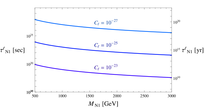
Figure 1: Partial lifetime of $N_{1}$ as a function of its mass $M_{N_{1}}$ and for selected values of the combination of mixing angles $C_{\ell}=\cos\theta\sin\theta_{\ell}$.

The primary $\ell^{\pm}$ and $W^{\mp}$, being the decay products of a particle nearly at rest, are practically monochromatic. In the approximation $m_{\ell}\ll M_{W}$, we have

$$p_{\ell}=E_{\ell}=\frac{M_{N_{1}}}{2}\left(1-\frac{M_{W}^{2}}{M_{N_{1}}^{2}}\right)=p_{W}~{}~{}~{},~{}~{}~{}~{}E_{W}=\frac{M_{N_{1}}}{2}\left(1+\frac{M_{W}^{2}}{M_{N_{1}}^{2}}\right)$$ (25)

where $p$ and $E$ denote particle’s momentum and energy, respectively.

The decaying heavy neutrinos $N_{1}$ are unpolarized, so the lepton $\ell$ and the $W$ bosons are emitted isotropically. Focusing on a single decay, it turns out that $\ell^{+}$ ($\ell^{-}$) is emitted preferentially in the same (opposite) direction as the $N_{1}$ spin. If the decaying $N_{1}$ has a TeV-scale mass, $\ell^{+}$ ($\ell^{-}$) is approximately an helicity eigenstate with eigenvalue $+1$ ($-1$). The associated $W$ boson can then be considered to be approximately an eigenstate of the component of the spin along its direction of motion with $0$ eigenvalue, that is to be longitudinally polarized.

III.2 Electron and positron energy spectra

Clearly, if $\ell^{\pm}$ is an unstable lepton like $\mu^{\pm}$ or $\tau^{\pm}$, it decays with a lifetime much shorter than $\tau_{N_{1}}$, producing $e^{\pm}$ and neutrinos. Also the associated $W^{\mp}$ boson quickly decays via electroweak interactions. Since we are interested in a TeV-scale $N_{1}$, its decay products are highly relativistic particles and we can safely work in the narrow-width approximation, i.e. we treat intermediate particles in fig. 2 as if they were on-shell. Accordingly, the number of $e^{\pm}$ per unit energy obtained from the decay of $N_{1}$ can be written as a sum of the contributions from the primary lepton and $W$ boson decay chains:

$$\frac{dN^{(\ell W)}(E_{e})}{dE_{e}}=\frac{1}{2}~{}\left(\frac{dN^{(\ell)}(E_{e})}{dE_{e}}+\frac{dN^{(W)}(E_{e})}{dE_{e}}\right)~{}~{},$$ (26)

where the factor $1/2$ has been introduced in order to fix the normalization of the separate contributions to one.

Figure 2: Example of charge conjugated Feynman diagrams for a cascade decay of $N_{1}$. Clearly, this is just a suggestive pictorial representation because $m_{\ell}>m_{\ell^{\prime}}>m_{\ell^{\prime\prime}}$ is realized only for $\tau,\mu,e$ respectively.

III.2.1 The lepton $\ell$ decay chain

Let analyse first the electrons and positrons coming from the primary $\ell$ decay chain.

• In this case, $e^{\pm}$ are monochromatic primary decay products of $N_{1}$, see eq.(25):

  $$\frac{dN^{(e)}(E_{e})}{dE_{e}}=\delta(E_{e}-\frac{M_{N_{1}}}{2}(1-\frac{M^{2}_{W}}{M^{2}_{N_{1}}}))~{}~{}.$$ (27)

  This is represented in the top right panel of fig. 3 as a vertical line.

• In this case, $e^{\pm}$ are produced as secondary decay products from the primary relativistic $\mu^{\pm}$ via its decay into $e^{\pm}\nu_{e}\nu_{\mu}$. They energy spectrum is thus continuous between $0\leq E_{e}\leq E_{\mu}$, as expected for the 3-body decay of a relativistic particle. Let take the $z$-axis to be parallel to the muon momentum. As already stressed, the spin of $\mu^{+}$ ($\mu^{-}$) is parallel (antiparallel) to $\hat{z}$. This means that the $\mu^{+}$ ($\mu^{-}$) is polarized in its rest frame, having spin parallel (antiparallel) to $\hat{z}$, so that the angular distribution of the outgoing $e^{+}$ ($e^{-}$) is enhanced in the same (opposite) direction as the muon spin, namely the $\hat{z}$ direction:

  $$\frac{d\tilde{\Gamma}_{\mu^{\pm}}}{d\cos\tilde{\theta}_{e^{\pm}}}=\frac{\tilde{\Gamma}_{\mu^{\pm}}}{2}(1+\frac{1}{3}\cos\tilde{\theta}_{e^{\pm}})$$ (28)

  where $\tilde{\theta}_{e^{\pm}}$ is the angle between $\hat{z}$ and the momentum of $e^{\pm}$ and quantities evaluated in the muon rest frame are indicated with a tilde. A relativistic $e^{\pm}$ produced in the rest frame of the $\mu^{\pm}$ with energy $\tilde{E}_{e^{\pm}}$, is found in the rest frame of $N_{1}$ to have an energy $E_{e^{\pm}}=\tilde{E}_{e^{\pm}}\gamma(1+\cos\tilde{\theta}_{e^{\pm}})$, with $\gamma=E_{\mu}/m_{\mu}$. As a result, the $e^{\pm}$ emitted with $\tilde{\theta}_{e^{\pm}}<\pi/2$ are slightly harder than for an unpolarized $\mu^{\pm}$ and, assuming $E_{\mu}\gg m_{\mu}$, their number per unit energy is given by

  $$\frac{dN^{(\mu^{\pm})}(E_{e^{\pm}})}{dE_{e^{\pm}}}=BR(\mu^{\pm}\rightarrow e^{\pm}\nu_{e}\nu_{\mu})~{}f_{\pm}(E_{\mu^{\pm}},E_{e^{\pm}},\pm 1)~{}~{},~{}~{}0\leq E_{e^{\pm}}\leq E_{\mu^{\pm}}~{}~{},$$ (29)

  where $E_{\mu^{\pm}}$ is the same as in eq.(25), the BR is close to $100\%$ and the function $f_{\pm}$ is defined as

  $$f_{\pm}(E_{i},E_{f},P_{i})=\frac{1}{3E_{i}}\left[5-9\left(\frac{E_{f}}{E_{i}}\right)^{2}+4\left(\frac{E_{f}}{E_{i}}\right)^{3}\mp P_{i}\left(1-9\left(\frac{E_{f}}{E_{i}}\right)^{2}+8\left(\frac{E_{f}}{E_{i}}\right)^{3}\right)\right]$$ (30)

  where $E_{i}$ and $E_{f}$ are the energy of the decaying and final lepton respectively and $P_{i}$ is the polarization of the decaying lepton (see e.g. Abreu:1995ku ). In our case $P_{\mu^{\pm}}=\pm 1$ and since $f_{+}(E_{i},E_{f},1)=f_{-}(E_{i},E_{f},-1)\equiv f(E_{i},E_{f})$, it can be directly checked that the energy distributions are equal for electrons and positrons, as expected. We then omit the apex $\pm$ and write explicitly

  $$\frac{dN^{(\mu)}(E_{e})}{dE_{e}}=f(E_{\mu},E_{e})~{}~{},~{}~{}f(E_{i},E_{f})=\frac{4}{3E_{i}}\left[1-\left(\frac{E_{f}}{E_{i}}\right)^{3}\right]~{}~{}.$$ (31)

  The energy distribution $dN^{(\mu)}(E_{e})/dE_{e}$ is represented with a dotted curve in the bottom left panel of fig.3, for $M_{N_{1}}=1,2,3,5$ TeV from top to bottom.

• In this case, there are both leptonic and hadronic decay modes, with BR of about $37\%$ and $63\%$ respectively.

  As for the leptonic decays, secondary $e^{\pm}$ are produced via $\tau^{\pm}\rightarrow e^{\pm}\nu_{e}\nu_{\tau}$ with an energy distribution similar to eq.(31) but suppressed because of the different BR

  $$\frac{dN^{(\tau/e)}(E_{e})}{dE_{e}}=BR(\tau\rightarrow e\nu_{e}\nu_{\tau})~{}f(E_{\tau},E_{e})~{}~{},~{}~{}0\leq E_{e}\leq E_{\tau}$$ (32)

  where $E_{\tau}$ is the same as in eq.(25) and the BR is about $17.8\%$. The primary $\tau^{\pm}$ decays also into $\mu^{\pm}\nu_{\mu}\nu_{\tau}$ with a similar BR. The latter $\mu^{\pm}$ has helicity close to $\pm 1$ and fully decays into $e^{\pm}\nu_{e}\nu_{\mu}$, giving an additional contribution to the energy distribution

  $$\frac{dN^{(\tau/\mu/e)}(E_{e})}{dE_{e}}=BR(\tau\rightarrow\mu\nu_{\mu}\nu_{\tau})~{}\int_{E_{e}}^{E_{\tau}}dE_{\mu}f(E_{\tau},E_{\mu})f(E_{\mu},E_{e})$$ (33)

  where $E_{\tau}$ is as in eq.(25) and $0\leq E_{e}\leq E_{\tau}$. The sum of the $e^{\pm}$ energy distributions resulting from $\tau^{\pm}$ leptonic decays is represented with a dash-dotted curve in the bottom right panel of fig.3, for $M_{N_{1}}=1,2,3,5$ TeV going from top to bottom. Notice that, because of the additional contribution from eq.(33), the dash-dotted curve is softer than the dotted one in the $\mu$ plot at left.

  Also the hadronic $\tau^{\pm}$ decay modes can produce $e^{\pm}$, which are generically softer than those produced in its leptonic decay modes. It is not difficult to give an estimate of their energy distribution. The $\tau^{\pm}$ decay modes into one or two pions are $\pi^{\pm}\nu_{\tau}$ and $\rho^{\pm}\nu_{\tau}\rightarrow\pi^{\pm}\pi^{0}\nu_{\tau}$, with BR$\approx 11\%$ and $25.5\%$ respectively. The $\pi^{\pm}$ then fully decays into $\mu^{\pm}\nu_{\mu}$. The $\tau^{\pm}$ decay modes into three or more pions have BR of about $26\%$ and can be neglected for the sake of the present analysis because the $e^{\pm}$ produced are very soft.

  Let study first the decay $\tau^{+}\rightarrow\pi^{+}\bar{\nu}_{\tau}$ ($\tau^{-}\rightarrow\pi^{-}\nu_{\tau}$). Since the $\tau^{+}$ ($\tau^{-}$) has helicity close to $+1$ ($-1$), in its rest frame it is approximately polarized with spin parallel (antiparallel) to $\hat{z}$, so that the pion momentum is mostly antiparallel to $\hat{z}$

  $$\frac{d\tilde{\Gamma}_{\tau}}{d\cos\tilde{\theta}_{\pi}}=\frac{\tilde{\Gamma}_{\tau}}{2}(1-\cos\tilde{\theta}_{\pi})~{}~{},$$ (34)

  where $\tilde{\theta}_{\pi}$ is the angle between $\hat{z}$ and the pion momentum in the pion rest frame. The pion mostly goes backwards with respect the the tau momentum and therefore it is softer than for an unpolarized tau decay. Indeed in the $N_{1}$ rest frame

  $$\frac{dN_{\tau}(E_{\pi})}{dE_{\pi}}=BR(\tau\rightarrow\pi\nu_{\tau})\frac{2}{p_{\tau}}\left(1-\frac{E_{\pi}}{E_{\tau}}\right)~{}~{}.$$ (35)

  The $\pi^{+}$ ($\pi^{-}$) decays isotropically in $\mu^{+}\nu_{\mu}$ ($\mu^{-}\bar{\nu}_{\mu}$), so that in the $N_{1}$ rest frame the muon has simply a flat energy distribution equal to $1/p_{\pi}\approx 1/E_{\pi}$. The $\mu^{+}$ ($\mu^{-}$) has approximately helicity $+1$ (-1) and fully decays into $e^{+}\nu_{e}\bar{\nu}_{\mu}$ ($e^{-}\bar{\nu}_{e}\nu_{\mu}$). The energy distribution of $e^{+}$ ($e^{-}$) is finally:

  $$\frac{dN^{(\tau/\pi/\mu/e)}(E_{e})}{dE_{e}}=\int_{E_{e}}^{E_{\tau}}dE_{\pi}\frac{dN_{\tau}(E_{\pi})}{dE_{\pi}}\int_{E_{e}}^{E_{\pi}}dE_{\mu}\frac{1}{p_{\pi}}f(E_{\mu},E_{e})~{}~{}.$$ (36)

  Secondly, we consider the decay $\tau^{+}\rightarrow\rho^{+}\bar{\nu}_{\tau}$ ($\tau^{-}\rightarrow\rho^{-}\nu_{\tau}$). The $\rho$ having spin $1$, it can take several polarization states and its angular distribution is less sensitive to the tau polarization

  $$\frac{d\tilde{\Gamma}_{\tau}}{d\cos\tilde{\theta}_{\rho}}=\frac{\tilde{\Gamma}_{\tau}}{2}(1-0.46\cos\tilde{\theta}_{\rho})~{}~{},$$ (37)

  but still the $\rho$ preferentially goes backwards with respect to the tau momentum and in the $N_{1}$ rest frame

  $$\frac{dN_{\tau}(E_{\rho})}{dE_{\rho}}=BR(\tau\rightarrow\rho\nu_{\tau})\frac{2}{p_{\tau}}\left(0.73-0.46\frac{E_{\rho}}{E_{\tau}}\right)~{}~{}.$$ (38)

  The $\rho^{\pm}$ is mildly polarized and it decays nearly isotropically in $\pi^{\pm}\pi^{0}$, with $\pi^{\pm}\rightarrow\mu^{\pm}\nu_{\mu}$. For the sake of the present analysis the electron energy distribution can be approximated by

  $$\frac{dN^{(\tau/\rho/\pi/\mu/e)}(E_{e})}{dE_{e}}=\int_{E_{e}}^{E_{\tau}}dE_{\rho}\frac{dN_{\tau}(E_{\rho})}{dE_{\rho}}\int_{E_{e}}^{E_{\rho}}dE_{\pi}\frac{1}{p_{\rho}}\int_{E_{e}}^{E_{\pi}}dE_{\mu}\frac{1}{p_{\pi}}f(E_{\mu},E_{e})~{}~{}.$$ (39)

  As already remarked, the remaining decays of the $\tau^{\pm}$ involve three or more pions in the final state: the $e^{\pm}$ eventually produced are even softer and can be neglected in the present analysis.

  The sum of the $e^{\pm}$ energy distributions resulting from $\tau^{\pm}$ leptonic and hadronic decays is represented with a dotted curve in the bottom right panel of fig.3, for $M_{N_{1}}=1,2,3,5$ TeV going from top to bottom. Clearly, the inclusion of the hadronic tau decay modes has the effect of softening the spectrum.

III.2.2 The $W$ boson decay chain

Also the primary and approximately linearly polarized $W$ boson further decays. The number of $e^{\pm}$ per unit energy produced in its decay chain has to be added to the ones studied above. The $W$ leptonic decay modes into pairs ${\ell}\nu_{\ell}$ have a BR of about $33\%$; the remaining $67\%$ is represented by hadronic decay modes. Let now identify direction of the $W$ momentum with the $\hat{z}$ axis.

As for the leptonic decay, in the $W$ rest frame (were the polarization vector is approximately $\vec{\epsilon}=i\hat{z}$) the secondary $\ell$ (see fig.2) is emitted with angular distribution given by:

$$\frac{d\tilde{\Gamma}_{W}}{d\cos\tilde{\theta}_{\ell}}=\frac{3\tilde{\Gamma}_{W}}{4}(1-\cos^{2}\tilde{\theta}_{\ell})~{}~{},$$ (40)

where $\tilde{\theta}_{\ell}$ is the angle between the $\hat{z}$ axis and the $\ell$ momentum. The lepton is preferentially emitted perpendicularly to $\hat{z}$ axis in the $W$ rest frame. In the $N_{1}$ rest frame it then displays an energy spectrum peaked at $E_{W}/2$:

$$\frac{dN_{W}(E_{\ell})}{dE_{\ell}}=BR(W\rightarrow{\ell}\nu_{\ell})\frac{6}{p_{W}}~{}\frac{E_{\ell}}{E_{W}}\left(1-\frac{E_{\ell}}{E_{W}}\right)~{}~{},~{}~{}0\leq E_{\ell}\leq E_{W}$$ (41)

where $p_{W}$ and $E_{W}$ are given in eq.(25) and we recall that the BR is roughly $11\%$ for all lepton flavors. At this point we have to sum over the flavors $\ell=e,\mu,\tau$. When $\ell=e$, its energy spectrum can be directly read out from eq.(41) above:

$$\frac{dN^{(W/e)}(E_{e})}{dE_{e}}=BR(W\rightarrow{e}\nu_{e})\frac{6}{p_{W}}~{}\frac{E_{e}}{E_{W}}\left(1-\frac{E_{e}}{E_{W}}\right)~{}~{},~{}~{}0\leq E_{e}\leq E_{W}~{}~{}.$$ (42)

When $\ell=\mu$, the contribution to the $e$ energy spectrum is given by

$$\frac{dN^{(W/\mu/e)}(E_{e})}{dE_{e}}=\int_{E_{e}}^{E_{W}}dE_{\mu}\frac{dN_{W}(E_{\mu})}{dE_{\mu}}f(E_{\mu},E_{e})~{}~{}.$$ (43)

When $\ell=\tau$, there is a similar but suppressed contribution

$$\frac{dN^{(W/\tau/e)}(E_{e})}{dE_{e}}=BR(\tau\rightarrow e\nu_{e}\nu_{\tau})\int_{E_{e}}^{E_{W}}dE_{\tau}\frac{dN_{W}(E_{\tau})}{dE_{\tau}}f(E_{\tau},E_{e})~{}~{}.$$ (44)

Since the $\tau$ also decays also into $\mu\nu_{\mu}\nu_{\tau}$, there is another small contribution from

$$\frac{dN^{(W/\tau/\mu/e)}(E_{e})}{dE_{e}}=BR(\tau\rightarrow\mu\nu_{\mu}\nu_{\tau})\int_{E_{e}}^{E_{W}}dE_{\tau}\frac{dN_{W}(E_{\tau})}{dE_{\tau}}\int_{E_{e}}^{E_{\tau}}dE_{\mu}f(E_{\tau},E_{\mu})f(E_{\mu},E_{e})~{}~{}.$$ (45)

Summarizing, for each primary $W^{\pm}$, the total number of $e^{\pm}$ produced in its leptonic decay modes is approximately $(11+11+2\times 0.17\times 11)\%\approx 1/4$.

The hadronic decays of the $W$ amounts to about $67\%$. They also can produce leptons, with a soft spectrum that is negligible for the sake of the present analysis.

In the top left panel of fig.3 we show the number of $e^{\pm}$ per unit energy produced by summing all the leptonic decays of the $W^{\pm}$ (the dotted line is the sole $\ell=e$ contribution), which has to be summed to the one coming from the primary $\ell^{\mp}$ and its eventual decays, as we are now going to discuss.

III.2.3 Results

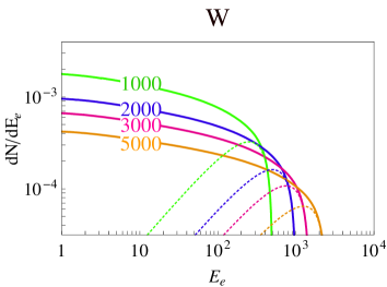
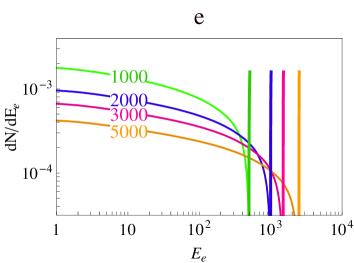
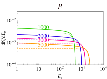
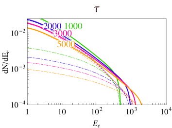
Figure 3: Number of $e^{\pm}$ per unit energy for selected values of $M_{N_{1}}$ in GeV. Top left: the solid lines are the total contribution from the $W$ boson leptonic decay chain; the dotted lines are the contribution from $W\rightarrow e\nu_{e}$ only. Top right: solid lines are the sum of the monochromatic $e$ and the $W$ chain. Bottom left: the solid lines are the sum of the $\mu$ and $W$ chains; the dotted ones are the contribution of the $\mu$ chain only. Bottom right: solid lines are the sum of the $\tau$ and $W$ chains; the dash-dotted lines are the contributions from the leptonic $\tau$ decays; the dotted lines the contribution from both leptonic and hadronic $\tau$ decays.

For each lepton flavor, we now sum the energy distributions of $e^{\pm}$ from the $\ell$ and $W$ boson chains.

For $\ell^{\pm}=e^{\pm}$, this sum is easily done since the primary $e^{\pm}$ are monochromatic, see the top right panel of fig.3.

For $\ell^{\pm}=\mu^{\pm}$, the energy spectrum of the secondary $e^{\pm}$ coming from its decay is soft. This is shown by the dotted curve in the left bottom panel of fig.3. The solid lines are obtained by adding the contribution of the $e^{\pm}$ coming from the $W$ chain. Since the $W$ chain provides approximately $25\%$ of the total number of $e^{\pm}$ produced in this decay of $N_{1}$, the contribution is small, especially for the hardest $e^{\pm}$.

For $\ell^{\pm}=\tau^{\pm}$, the energy spectrum of the $e^{\pm}$ coming from its leptonic decay is also soft, but suppressed because of the BR of about $34\%$, as can be seen from the dash-dotted curves in the right bottom panel of fig.3. The dotted line are obtained by adding the contribution from the $\tau$ hadronic decay. Finally, the solid lines are obtained by adding also the contribution from the $W$ chain, which is relevant at the highest energies and hardens the spectrum close to its end point.

III.3 Contributions to $e^{\pm}$ CR’s

Having obtained explicit expressions for the number of electrons and positrons per unit energy produced via each channel $N_{1}\rightarrow\ell W$ and its subsequent decays, it is straightforward to substitute them into eq.(20) and to calculate the flux observed at Earth

$$\phi(E_{e})=\sum_{\ell}\phi^{\ell}(E_{e})~{}~{},~{}~{}\phi^{\ell}(E_{e})=\frac{c}{4\pi}f^{\ell}_{e}(E_{e})~{}~{},$$ (46)

where $c$ is the speed of light.

Clearly, because of the propagation in the galaxy, the energy spectrum of the electrons and positrons gets modified according to the diffusion equation. The solid lines in the three panels of fig.4 display the combination $E_{e}^{3}\phi^{\ell}(E_{e})$ for each lepton flavour, by assuming $C_{\ell}x_{N_{1}}^{1/2}=10^{-27}$ and for four selected values of $M_{N_{1}}$ in GeV. We recall that the fluxes are proportional to $C_{\ell}^{2}$. It is thus not difficult to obtain the total flux $\phi(E_{e})$ corresponding to any possible set of $C_{e},C_{\mu}$ and $C_{\tau}$. The dotted line are obtained by neglecting the contribution of electrons and positrons originated from the $W$ boson chain. The spectrum turns out to be hard for $\ell=e$, while it is softer for $\ell=\mu$, and even more for $\ell=\tau$.

Notice that energy losses due to the diffusion in the galaxy are more relevant at low rather than at high $E_{e}$. This can be realized by comparing, for instance, the plots for the muon case: the value of the flux increases with $M_{N_{1}}$ in the whole energy range, while this was not the case for the number of electrons and positrons per unit energy at the source, see fig.3. The same applies for the tau case, for which the energy spectrum at the source is even softer. This justifies the fact that in our calculation we neglected the softer electrons and positrons coming from the hadronic $\tau$ decays with more than three pions, as well as those coming from the hadronic decays of the $W$. Fig.4 show indeed that the shape of the fluxes after propagation is essentially controlled by the behaviour of $dN/dE_{e}$ close to its end point (i.e. for the highest possible values of $E_{e}$). For the muon case, this behaviour is a direct reflection of eq.(31); for the tau, of the sum of eqs.(32),(33) and (42).

The same argument can be applied to electroweak radiation effectsCirelli:2010xx ; Ciafaloni:2010ti . Since the mass scale of the Majorana neutrino $N_{1}$ is much bigger than the electroweak scale, soft electroweak vector bosons can be radiated in its decay. Such vector boson give even softer electrons and positrons, they can be neglected in the present analysis because the cosmic ray excesses observed by PAMELA and Fermi-LAT are comprised in the energy range from $20$ GeV to $1$ TeV.

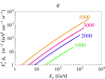
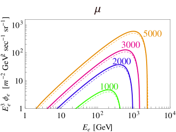
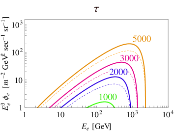
Figure 4: Flux of $e^{\pm}$ multiplied by $E_{e}^{3}$ for $N_{1}\rightarrow\ell W$ with $\ell=e,\mu,\tau$ respectively and for $M_{N_{1}}=1000,2000,3000,5000$ GeV. The dashed line is obtained neglecting the contribution from the $W$ chain. We fixed $C_{\ell}x_{N_{1}}^{1/2}=10^{-27}$ everywhere.

IV Comparison between the model and the data by PAMELA and Fermi-LAT

We now come to the comparison between our fourth lepton family model with a decaying TeV-scale Majorana neutrino and the experimental data on $e^{\pm}$ CRs recently collected by PAMELA and Fermi-LAT. We will first describe an extremely fast method, based on the Sum Rules (SR) introduced in ref.Frandsen:2010mr . This method allows for a fast scrutiny of the viability of any model (we considered in particular the case of models predicting an equal amount of fluxes for electrons and positrons, but the method could of course be generalized). Then, we go through the longer path of the direct comparison, also to show the reliability of the SR method.

IV.1 Sum Rules method

A fast method to check the viability of our model is to make use of the results of ref.Frandsen:2010mr , that we briefly summarize here. For definiteness and also for an easy comparison with the literature, let consider the Moskalenko Strong (MS) Strong:1998pw ; Baltz:1998xv fluxes $B^{\pm}(E_{e})$, where $\pm$ refer to positrons and electrons respectively, to model the contribution of astrophysical sources (one could of course apply the same reasoning for any other astrophysical background model), leaving the normalization of the fluxes $N_{B}$ as a free parameter: $\phi_{\pm}^{B}(E_{e})=N_{B}B^{\pm}(E_{e})$.

We assume that an unknown source of $e^{\pm}$ CR is also present, which gives equal fluxes for electrons and positrons, $\phi_{+}^{U}(E_{e})=\phi_{-}^{U}(E_{e})\equiv\phi^{U}(E_{e})$. Hence the total fluxes are

$$\phi_{+}(E_{e})=\phi^{U}(E_{e})+\phi_{+}^{B}(E_{e})~{}~{},~{}~{}\phi_{-}(E_{e})=\phi^{U}(E_{e})+\phi_{-}^{B}(E_{e})~{}~{}.$$ (47)

In ref.Frandsen:2010mr we showed how to combine the PAMELA and Fermi-LAT data in order to extrapolate the flux of $e^{\pm}$ from this unknown source. We re-display this flux $\phi^{U}(E_{e})$ in fig. 5, by means of the shaded region. The inner and outer bands have been obtained by combining respectively the $1\sigma$ and $2\sigma$ error bands of PAMELA and Fermi-LAT, while considering all possible associated values for $N_{B}$ by means of the SR.

It is now straightforward to compare the experimentally extrapolated flux $\phi^{U}(E_{e})$ with our particular model, belonging indeed to the category of models which predict equal fluxes for the electrons and positrons. All we have to do is to superimpose the (solid) curves of the fluxes already shown in fig.4. This is done in fig. 5, where the $C_{\ell}$’s have been fixed so to cross the shaded region at the lowest energies. We recall that the fluxes scale as $C_{\ell}^{2}$, so that it is not difficult to obtain the value of the fluxes for any other value of $C_{\ell}$. The dashed curves have been obtained by neglecting polarization effects in both $\ell$ and $W$ decay chains.

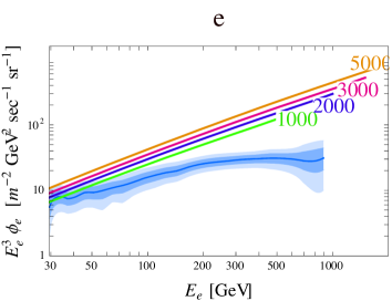
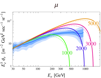
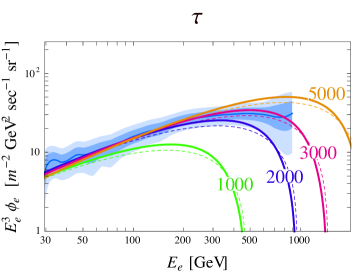
Figure 5: Comparison between the prediction of our model for selected values of $M_{N_{1}}$ in GeV and the combined data from PAMELA and Fermi-LAT Frandsen:2010mr . The inner and outer bands have been obtained by combining respectively the $1\sigma$ and $2\sigma$ error bands of PAMELA and Fermi-LAT (2010 releases), together with the MS model for the astrophysical background. For $M_{N_{1}}=3$ TeV, the curves have been obtained by setting $C_{e}x_{N_{1}}^{1/2}=10^{-27.02}$, $C_{\mu}x_{N_{1}}^{1/2}=10^{-27.11}$ and $C_{\tau}x_{N_{1}}^{1/2}=10^{-27.05}$. Solid (dashed) lines display the results of including (neglecting) polarization effects.

We can see that the electron and positron fluxes obtained via the mixing of $N_{1}$ and the $e$-flavor charged lepton have not the right spectral index to fit the combined experimental data. In the case of mixing with the muon, the electron and positron fluxes follow the shape of the data quite well for values of $N_{1}$ close to $2-3$ TeV. For the mixing with tau, the agreement is even more impressive. For $M_{N_{1}}=3$ TeV, the curves have been obtained by setting $C_{e}x_{N_{1}}^{1/2}=10^{-27.02}$, $C_{\mu}x_{N_{1}}^{1/2}=10^{-27.11}$ and $C_{\tau}x_{N_{1}}^{1/2}=10^{-27.05}$.

This means that, if we want to interpret the PAMELA and Fermi-LAT excesses as being due to a decaying heavy Majorana neutrino, we need $M_{N_{1}}\approx 3$ TeV, $C_{\tau}x_{N_{1}}^{1/2}\approx 10^{-27}$ and/or $C_{\mu}x_{N_{1}}^{1/2}\approx 10^{-27}$ while $C_{e}x_{N_{1}}^{1/2}\lesssim 10^{-28}$. Hence the hierarchy $\theta_{e}<\theta_{\mu,\tau}$ among the mixing angles with the light leptons is needed.

The universal coupling case $\theta_{e}=\theta_{\mu}=\theta_{\tau}$ is thus excluded, as already pointed out by the numerical analysis of ref.Ibarra:2009dr , where a generic heavy fermion decaying into $\ell W$ was considered (the nature of the vertex interaction was not specified). We postpone to the next section a more complete comparison with previous analysis.

IV.2 Direct method

We now come to the direct comparison between our fourth lepton family model with a decaying TeV-scale Majorana neutrino, considering separately the PAMELA and Fermi-LAT experimental data on $e^{\pm}$ CRs.

The fluxes of $e^{\pm}$ arising from $N_{1}$ decays that we come to calculate have to be summed to those arising from astrophysical sources. As before, we consider the popular MS model Strong:1998pw ; Baltz:1998xv for such astrophysical background and recall the explicit expressions for $B^{\pm}(E)$:

$$B^{+}(E) = \frac{4.5E^{0.7}}{1+650E^{2.3}+1500E^{4.2}}\ ,$$ (48)

$$B^{-}(E) = B_{1}^{-}+B_{2}^{-}\ ,$$ (49)

$$B_{1}^{-}(E) = \frac{0.16E^{-1.1}}{1+11E^{0.9}+3.2E^{2.15}}\ ,$$ (50)

$$B_{2}^{-}(E) = \frac{0.70E^{0.7}}{1+110E^{1.5}+600E^{2.9}+580E^{4.2}}\ ,$$ (51)

where $E$ is measured in ${\rm GeV}$ and the $B$s in ${\rm GeV}^{-1}{\rm cm}^{-2}{\rm sec}^{-1}{\rm sr}^{-1}$ units. To be specific, in the present analysis we fix the value $N_{B}=0.638$, obtained by means of the sum rule method proposed in ref.Frandsen:2010mr .

We start by considering the positron fraction and display it in the left panels of fig. 6 for $\ell=e,\mu,\tau$ respectively and for selected values of the $N_{1}$ mass, $M_{N_{1}}=1,2,3,5$ TeV. Solid (dashed) curves have been obtained by including (neglecting) polarization effects. The panels also show the PAMELA $1\sigma$ data points (2010 release) and the MS model prediction. The mixing angle $C_{\ell}$ has been chosen so that our model curves cross the central value of the PAMELA positron fraction data point associated to the $35$ GeV energy bin, $\phi_{e^{+}}/(\phi_{e^{-}}+\phi_{e^{+}})=0.733$. Notice that $C_{\ell}$ plays the role of shifting up and down the curves with respect to MS. The shape of the curves depends on the value of $M_{N_{1}}$, since they drop at about $M_{N_{1}}/2$. The dropping is sharp for $\ell=e$, soft for $\mu$ and even softer for $\tau$. This pattern clearly reflects the shape of the fluxes displayed in fig.4. It can be realized that the PAMELA data points are nicely fitted for any value of $M_{N_{1}}$, provided it is bigger than about $200$ GeV Nardi:2008ix .

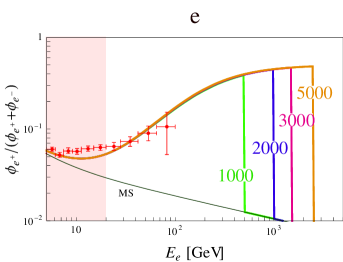
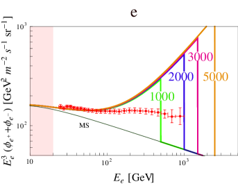
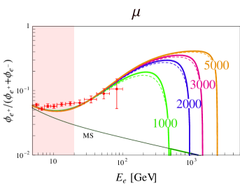
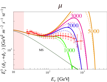
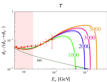
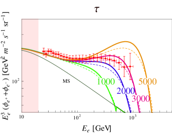
Figure 6: Comparison with the 2010 releases of PAMELA (left) and Fermi-LAT (right), considering separately the mixing between $N_{1}$ and each SM lepton $\ell=e,\mu,\tau$. The value of the $C_{\ell}$ fits the central value of the PAMELA $35$ GeV data point. The solid lines correspond to $M_{N_{1}}=1,2,3,5$ TeV from bottom to top respectively. The shaded region emphasizes the energy range where solar modulation effects cannot be neglected. The bottom black line displays the MS estimate for the astrophysical backgrounds. For $M_{N_{1}}=3$ TeV, the values used in the plot for $\log_{10}(C_{\ell}x_{N_{1}}^{1/2})$ are $-27.105,-27.112,-27.031$ respectively for $e,\mu,\tau$. Solid (dashed) lines display the results of including (neglecting) polarization effects.

This does not happen for the Fermi-LAT data on the total electron and positron flux, as shown in the right panels of fig. 6 for $\ell=e,\mu,\tau$ respectively. The couplings $C_{\ell}$ have been chosen to be the same as the corresponding ones in the PAMELA plots at the left. Again, solid (dashed) curves have been obtained by including (neglecting) polarization effects. It is evident that the Fermi-LAT data points cannot be fitted for $\ell=e$, since the curves raise too much. For $\ell=\tau$ the curves have a shape that is nicely compatible with the data for values of $M_{N_{1}}$ close to $2-3$ TeV, while for $\ell=\mu$ there is some tension because of an excess around $500-1000$ GeV. For $M_{N_{1}}=3$ TeV, the values of the combination $\log_{10}(C_{\ell}x_{N_{1}}^{1/2})$ used in the plot are $-27.105,-27.112,-27.031$ respectively for $e,\mu,\tau$. This means that, if we want to interpret the PAMELA and Fermi-LAT excesses as being due to a decaying heavy Majorana neutrino, we need $\theta_{e}<\theta_{\mu,\tau}$, as concluded in the previous section.

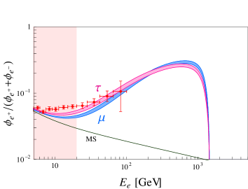
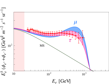
Figure 7: Our best fits of PAMELA (left) and Fermi-LAT (right) data. The mass of $N_{1}$ has been chosen to be $3$ TeV. In the upper (lower) panels polarization effects have been included (neglected). For $N_{1}\rightarrow\tau W$ we used $x_{N_{1}}^{1/2}C_{\tau}=10^{-27.07}-10^{-27.02}$, while for $N_{1}\rightarrow\mu W$ we used $x_{N_{1}}^{1/2}C_{\mu}=10^{-27.25}-10^{-27.20}$. In the upper panels polarizations effects are included, in the lower panels they are neglected.

As already stressed, the curve for $\tau$ is slightly softer than for $\mu$ because the its energy spectrum is slightly softer, see fig.3 and 4. The excess of the $\mu$ curves at $2-3$ TeV could be easily corrected for by slightly reducing the coupling $C_{\mu}$. This is demonstrated in fig.7 where we show the best fit values of $C_{\ell}$ for $\ell=\mu$ and $\tau$ and for $M_{N_{1}}=3$ TeV. We can see that the $\tau$ fits astonishingly well both PAMELA and Fermi-LAT data with $x_{N_{1}}^{1/2}C_{\tau}=10^{-27.07}-10^{-27.02}$. The fit for the muon with a slightly suppressed coupling, $x_{N_{1}}^{1/2}C_{\mu}=10^{-27.25}-10^{-27.20}$, is now good. Clearly, we were able to conclude all this also by means of the SR method discussed previously. However, the direct analysis allows for a better comparison with the results of ref.Ibarra:2009dr , as we now turn to discuss. Polarization effects have been included in the upper panels, while they have been neglected in the lower panels. The inclusion of polarization slightly hardens the total flux.

Ref.Ibarra:2009dr concluded that the $\tau W$ channel does not fit the Fermi-LAT data because of a too much flat curve; their best fit was obtained in the case of the $\mu W$ channel. Indeed, in their plots the fluxes appear softer for both $\mu W$ and $\tau W$ as compared to fig.7, even neglecting polarization effects; the latter is in particular so soft that the agreement with the Fermi-LAT experimental data is lost. In ref. Meade:2009iu the $\tau W$ mode was considered to provide a good fit of the data, but worse than the $\mu W$ mode. We suspect that the discrepancy with previous numerical analysis could either be due to a vertex interaction different from eq.(1) (for instance including all chiralities) or to their numerical code. Their analysis is based on PYTHIA, that treats leptons and vector bosons as unpolarized. However, as diplayed in fig.7, the inclusion of polarization effects cannot alone explain the discrepancy.

The hardness of the upper right panel spectra for $\mu$ and $\tau$ follows directly from the fact that the CC vertex involves L-handed (R-handed) leptons (antileptons). If we had considered a non chiral vertex or if we had neglected polarization effects in our calculation, the curves in fig.7 would have been softer, as demonstrated in the lower right panel. This can be easily understood for the $\mu$ case, since the contribution from the $W$ decay chain is negligible and the shape of the flux in fig.7 is essentially controlled by the energy distribution of the $e^{\pm}$ produced in the $\mu^{\pm}$ decay, eq.(31). For instance, for a relativistic L-handed $\mu^{-}$, the highest energy $e^{-}$ produced in its decay are slightly harder than in the unpolarized case because they are preferentially produced with momentum parallel to the muon one, eq. (28). At the contrary, for relativistic R-handed $\mu^{-}$, the highest energy electrons preferentially escape with opposite momentum and are thus softer.

V Cosmic Ray Antiprotons

In this section we give an estimate for the cosmic ray antiproton flux resulting from the heavy Majorana neutrino decay and compare it with current data.

Protons and antiprotons are generated via the hadronic decay of the primary $W$ boson, with BR of about $67\%$. Their energy spectrum is determined by the fragmentation and hadronization processes. In this case an analytic approach is not suitable and we rather adopt the numerical recipies provided in ref. Cirelli:2010xx . In particular, the antiproton (proton) flux obtained from a $1.5$ TeV dark matter annihilating into $W^{+}W^{-}$ is twice the antiproton (proton) flux in our model.

The propagation for antiprotons through the galaxy is described by a diffusion equation whose solution can be cast in a factorized form as discussed e.g. in Cirelli:2010xx . In this case the astrophysical uncertainties associated to the dark matter profile and to the propagation parameters are large, about one order of magnitude. We display the antiproton flux in the left panel of fig. 8 for the MAX, MED, MIN propagation models and for $M_{N_{1}}=3$ TeV and $x_{N_{1}}^{1/2}C_{\ell}=10^{-27.2}$. The dashed curves show these primary antiprotons for MAX, MED, MIN models; the lower shaded region represents the flux of the secondary antiprotons according to ref.Bringmann:2006im ; the upper three curves correspond to the sum of the primary and secondary antiprotons. The (lower) PAMELA data Adriani:2010rc have smaller error bars with respect to the (upper) CAPRICE data Boezio:2001ac . It turns out that only the MIN propagation parameter set is compatible with the data, the MED one is barely compatible, while the MAX seems disfavored.

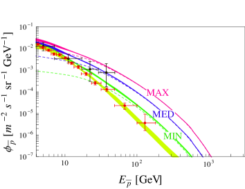
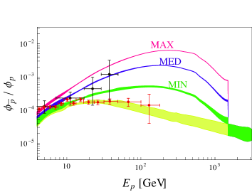
Figure 8: Antiproton flux (left) and antiproton/proton ratio (right) for the MAX, MED, MIN propagation models, $M_{N_{1}}=3$ TeV and $x_{N_{1}}^{1/2}C_{\ell}=10^{-27.2}$. The dashed curves in the left panel show the primary antiprotons for MAX, MED, MIN models. The lower shaded region represents the secondary antiprotons only, according to ref.Bringmann:2006im . The upper three curves correspond to the sum of the primary and secondary antiprotons. The (lower) PAMELA data Adriani:2010rc have smaller error bars with respect to the (upper) CAPRICE data Boezio:2001ac .

The antiproton/proton ratio is studied in the right panel of fig.8. For the proton flux, we consistently adopt the parameterization of ref.Bringmann:2006im with spectral index equal to $-2.72$. This parameterization is valid for energies higher than about $10$ GeV. Again, the (lower) PAMELA data points Adriani:2010rc are more precise than the (upper) CAPRICE ones Boezio:2001ac . The plot shows that even the MIN model displays tension with the PAMELA data. Future measurements confirming the PAMELA results could be able to rule out the heavy decaying neutrino model studied in this work.

VI Conclusions

In this work we have asked whether the electron and positron CR excesses observed by PAMELA and Fermi-LAT can be produced by a decaying fourth lepton family Majorana neutrino $N_{1}$. Several more or less natural models of Majorana neutrino dark matter have been put forward in the literature in addition to the ones cited in this work. A review of different models is Fan:2010yq . We note, however, that our model of Majorana neutrino emerges naturally at the electroweak scale given that the new generation of leptons is needed to resolve the Witten anomaly associated to the specific technicolor extension known as Minimal Walking Technicolor Sannino:2004qp ; Dietrich:2005jn ; Foadi:2007ue . We have already investigated the collider properties of our extension in Frandsen:2009fs . There we have also discussed and compared with other models of fourth family of leptons at the electroweak scale.

This heavy neutrino mixes only with the SM charged leptons via CC interactions, so its primary decay products are $\ell W$, $\ell=e,\mu,\tau$, with BR proportional to the combination $C_{\ell}^{2}/(C_{e}^{2}+C_{\mu}^{2}+C_{\tau}^{2})$, where $C_{\ell}$ represents the strength of the mixing between $N$ and the SM charged lepton $\ell$. If the mixing angles are sufficiently small, $N_{1}$ is nearly stable on cosmological time scales and constitutes a fraction $x_{N_{1}}$ of the today dark matter density.

We analytically calculated the energy spectrum of the electrons and positrons produced via the decay channel $\ell W$ and its subsequent decays, including polarization effects. The shape of the energy spectrum is different for $\ell=e,\mu,\tau$, as can be seen in fig.3.

After propagation (here we adopted the approximation of Ibarra:2008qg for the Green function of the MED-model Delahaye:2007fr ) the contribution to the total flux from each decay channels can be straightforwardly compared with the PAMELA and Fermi-LAT experimental data combined according to the Sum Rules method Frandsen:2010mr , see fig.5. We also carried out the more standard method of the separate comparison between the PAMELA and Fermi-LAT data in order to show the reliability of the SR method.

Our results are that the model provide a plausible explanation of the observed CRs excesses, when the BRs of $N_{1}\rightarrow\tau W$ and $N_{1}\rightarrow\mu W$ are the dominant ones, as it is clear from fig. 7. No acceptable agreement with the data can be achieved for $N_{1}\rightarrow eW$. This means that $N_{1}$ should have a hierarchical pattern of mixing angles with the SM charged leptons, with $C_{e}<C_{\mu,\tau}$. In particular, the $\tau W$ decay mode alone seems to best fit the data. In this case, the best fit occurs for $M_{N_{1}}\approx 3$ TeV and $\sqrt{x_{N_{1}}}C_{\tau}\approx 10^{-27}$. For the $\tau W$ decay our results differ from the ones obtained in ref.Ibarra:2008qg ; Meade:2009iu by using numerical codes. We found that our inclusion of polarization effects cannot alone explain this discrepancy.

We have demonstrated that the positron and electron CR excesses possibly present in the PAMELA and Fermi-LAT data, can be simply accounted for in our fourth generation heavy Majorana neutrino model. Clearly, the contraints from gamma photons Abdo:2010ex ; Abdo:2010nz would deserve a dedicated analysis, but we do not expect to find tension between our model and these data. We instead estimated the primary contribution to the antiproton flux and the antiproton to proton ratio in our model. Despite the uncertainty in the propagation parameters, it seems that even the MIN model shows tension with the PAMELA data Adriani:2010rc . The AMS-02 space station experiment will hopefully provide additional relevant informations ams02 .

Appendix A Full mixing

The mixing between the neutrinos of flavor $\zeta$ and the three SM neutrinos is described by the $5\times 5$ mass matrix ${\cal M}$:

$$-{\cal L}=\frac{1}{2}(\begin{array}[]{ccccc}\overline{(\nu_{eL})^{c}}&\overline{(\nu_{\mu L})^{c}}&\overline{(\nu_{\tau L})^{c}}&\overline{(\nu_{\zeta L})^{c}}&\overline{\nu_{\zeta R}}\end{array})\left(\begin{array}[]{ccc|cc}{\cal O}(eV)&{\cal O}(eV)&{\cal O}(eV)&{\cal O}(eV)&m_{e}\cr{\cal O}(eV)&{\cal O}(eV)&{\cal O}(eV)&{\cal O}(eV)&m_{\mu}\cr{\cal O}(eV)&{\cal O}(eV)&{\cal O}(eV)&{\cal O}(eV)&m_{\tau}\cr\hline\cr{\cal O}(eV)&{\cal O}(eV)&{\cal O}(eV)&{\cal O}(eV)&m_{D}\cr m_{e}&m_{\mu}&m_{\tau}&m_{D}&m_{R}\end{array}\right)\left(\begin{array}[]{c}\nu_{eL}\cr\nu_{\mu L}\cr\nu_{\tau L}\cr\nu_{\zeta L}\cr(\nu_{\zeta R})^{c}\end{array}\right)+h.c.~{}~{}.$$ (52)

Barring unnatural tunings and up to corrections to its mixings of ${\cal O}(eV/M_{N_{1},N_{2}})$, the unitary matrix $V$ is

$$\left(\begin{array}[]{c}\nu_{eL}\cr\nu_{\mu L}\cr\nu_{\tau L}\cr\nu_{\zeta L}\cr(\nu_{\zeta R})^{c}\end{array}\right)=V\left(\begin{array}[]{c}P_{L}N_{e}\cr P_{L}N_{\mu}\cr P_{L}N_{\tau}\cr P_{L}N_{1}\cr P_{L}N_{2}\end{array}\right)~{}~{},~{}~{}V=\left(\begin{array}[]{ccccc}c_{e}&0&0&ics_{e}&ss_{e}\cr-s_{e}s_{\mu}&c_{\mu}&0&icc_{e}s_{\mu}&sc_{e}s_{\mu}\cr-s_{e}c_{\mu}s_{\tau}&-s_{\mu}s_{\tau}&c_{\tau}&icc_{e}c_{\mu}s_{\tau}&sc_{e}c_{\mu}s_{\tau}\cr-s_{e}c_{\mu}c_{\tau}&-s_{\mu}c_{\tau}&-s_{\tau}&icc_{e}c_{\mu}c_{\tau}&sc_{e}c_{\mu}c_{\tau}\cr 0&0&0&-is&c\end{array}\right)~{},$$ (53)

where

$$t_{\tau}^{2} = \frac{{m}_{\tau}^{2}}{m_{D}^{2}}~{}~{}~{},~{}~{}~{}~{}~{}~{}t_{\mu}^{2}=\frac{{m}_{\mu}^{2}}{m_{D}^{2}+{m}_{\tau}^{2}}~{}~{}~{},~{}~{}~{}~{}~{}t_{e}^{2}=\frac{{m}_{e}^{2}}{m_{D}^{2}+{m}_{\tau}^{2}+{m}_{\mu}^{2}}~{}~{},$$

$$~{}~{}~{}~{}~{}~{}\tan(2\theta)=2~{}\frac{{m^{\prime}}_{D}}{m_{R}}~{}~{},~{}~{}~{}{m^{\prime}}_{D}^{2}=m_{D}^{2}+{m}_{\tau}^{2}+{m}_{\mu}^{2}+{m}_{e}^{2},$$

diagonalises the lower $2\times 2$ sector of the $5\times 5$ mass matrix ${\cal M}$, namely

$$V{\cal M}V^{\dagger}=\left(\begin{array}[]{ccc}m^{eff}_{3\times 3}&0&0\cr 0&M_{N_{1}}&0\cr 0&0&M_{N_{2}}\end{array}\right)$$ (55)

where the elements of $m^{eff}_{3\times 3}$ are naturally ${\cal O}(eV)$ and

$$M_{N_{1}}=\frac{m_{R}}{2}\left(\sqrt{1+4\frac{{m^{\prime}_{D}}^{2}}{m_{R}^{2}}}-1\right)~{}~{},~{}~{}~{}~{}M_{N_{2}}=\frac{m_{R}}{2}\left(\sqrt{1+4\frac{{m^{\prime}_{D}}^{2}}{m_{R}^{2}}}+1\right)~{}.$$ (56)

At this stage, the matrix in eq.(55) can be fully diagonalised with a further unitary matrix, which can be identified with the MNS mixing matrix, acting only on the upper $3\times 3$ block:

$$U^{\dagger}m^{eff}_{3\times 3}U^{*}={\rm diag}(m_{1},m_{2},m_{3})~{}~{}.$$ (57)

Notice that in the limit of small mixing angles between the heavy and light neutrinos, the mixing matrix $V$ becomes (at first order in $s_{\ell}$)

$$V\approx\left(\begin{array}[]{ccccc}1&0&0&ics_{e}&ss_{e}\cr 0&1&0&ics_{\mu}&ss_{\mu}\cr 0&0&1&ics_{\tau}&ss_{\tau}\cr-s_{e}&-s_{\mu}&-s_{\tau}&ic&s\cr 0&0&0&-is&c\end{array}\right)~{}.$$ (58)

We have thus demonstrated that each light flavor couples to the heavy neutrinos as in eq.(12).

References

- (1) O. Adriani et al. [PAMELA Collaboration], “An anomalous positron abundance in cosmic rays with energies 1.5-100 GeV, Nature 458 (2009) 607 [arXiv:0810.4995 [astro-ph]]. O. Adriani et al. [PAMELA Collaboration], A statistical procedure for the identification of positrons in the PAMELA experiment, Astropart. Phys. 34 (2010) 1 [arXiv:1001.3522 [astro-ph.HE]].
- (2) A. A. Abdo et al. [Fermi LAT Collaboration], Measurement of the Cosmic Ray e+ plus e- spectrum from 20 GeV to 1 TeV with the Fermi Large Area Telescope, Phys. Rev. Lett. 102 (2009) 181101 [arXiv:0905.0025 [astro-ph.HE]]. M. Ackermann et al. [Fermi LAT Collaboration], Fermi LAT observations of cosmic-ray electrons from 7 GeV to 1 TeV, Phys. Rev. D 82 (2010) 092004 [arXiv:1008.3999 [astro-ph.HE]].
- (3) J. Chang et al. [ATIC Collaboration], An Excess Of Cosmic Ray Electrons At Energies Of 300-800 Gev, Nature 456 (2008) 362.
- (4) S. Torii et al. [PPB-BETS Collaboration], High-energy electron observations by PPB-BETS flight in Antarctica, arXiv:0809.0760 [astro-ph].
- (5) F. Aharonian et al. [H.E.S.S. Collaboration], The energy spectrum of cosmic-ray electrons at TeV energies, Phys. Rev. Lett. 101 (2008) 261104 [arXiv:0811.3894 [astro-ph]]. F. Aharonian et al. [H.E.S.S. Collaboration], Probing the ATIC peak in the cosmic-ray electron spectrum with H.E.S.S, Astron. Astrophys. 508 (2009) 561 [arXiv:0905.0105 [astro-ph.HE]].
- (6) O. Adriani et al. [PAMELA Collaboration], PAMELA results on the cosmic-ray antiproton flux from 60 MeV to 180 GeV in kinetic energy, Phys. Rev. Lett. 105 (2010) 121101 [arXiv:1007.0821 [astro-ph.HE]]. See also: O. Adriani et al., A new measurement of the antiproton-to-proton flux ratio up to 100 GeV in the cosmic radiation, Phys. Rev. Lett. 102 (2009) 051101 [arXiv:0810.4994 [astro-ph]].
- (7) Y. -Z. Fan, B. Zhang, J. Chang, Excesses in the Cosmic Ray Spectrum and Possible Interpretations, Int. J. Mod. Phys. D19 (2010) 2011-2058. [arXiv:1008.4646 [astro-ph.HE]].
- (8) E. Nardi, F. Sannino and A. Strumia, Decaying Dark Matter can explain the electron/positron excesses, JCAP 0901 (2009) 043 [arXiv:0811.4153 [hep-ph]].
- (9) A. Ibarra, D. Tran and C. Weniger, Detecting Gamma-Ray Anisotropies from Decaying Dark Matter: Prospects for Fermi LAT, Phys. Rev. D 81 (2010) 023529 [arXiv:0909.3514 [hep-ph]].
- (10) M. Cirelli, P. Panci and P. D. Serpico, Diffuse gamma ray constraints on annihilating or decaying Dark Matter after Fermi, Nucl. Phys. B 840 (2010) 284 [arXiv:0912.0663 [astro-ph.CO]].
- (11) P. Meade, M. Papucci, A. Strumia and T. Volansky, Dark Matter Interpretations of the Electron/Positron Excesses after FERMI, Nucl. Phys. B 831 (2010) 178 [arXiv:0905.0480 [hep-ph]].
- (12) M. Papucci and A. Strumia, Robust implications on Dark Matter from the first FERMI sky gamma map, JCAP 1003 (2010) 014 [arXiv:0912.0742 [hep-ph]].
- (13) G. Hutsi, A. Hektor and M. Raidal, Implications of the Fermi-LAT diffuse gamma-ray measurements on annihilating or decaying Dark Matter, JCAP 1007 (2010) 008 [arXiv:1004.2036 [astro-ph.HE]].
- (14) C. Boehm, T. Delahaye and J. Silk, Can the morphology of gamma-ray emission distinguish annihilating from decaying dark matter?, Phys. Rev. Lett. 105 (2010) 221301 [arXiv:1003.1225 [astro-ph.GA]].
- (15) S. Palomares-Ruiz and J. M. Siegal-Gaskins, Annihilation vs. Decay: Constraining Dark Matter Properties from a Gamma-Ray Detection in Dwarf Galaxies, arXiv:1012.2335 [astro-ph.CO].
- (16) F. Sannino and K. Tuominen, Techniorientifold, Phys. Rev. D 71, 051901 (2005) [arXiv:hep-ph/0405209].
- (17) D. D. Dietrich, F. Sannino and K. Tuominen, “Light composite Higgs from higher representations versus electroweak precision measurements: Predictions for CERN LHC,” Phys. Rev. D 72, 055001 (2005) [arXiv:hep-ph/0505059].
- (18) R. Foadi, M. T. Frandsen, T. A. Ryttov and F. Sannino, “Minimal Walking Technicolor: Set Up for Collider Physics,” Phys. Rev. D 76, 055005 (2007) [arXiv:0706.1696 [hep-ph]].
- (19) M. T. Frandsen, I. Masina and F. Sannino, Fourth Lepton Family is Natural in Technicolor, Phys. Rev. D 81, 035010 (2010) [arXiv:0905.1331 [hep-ph]].
- (20) O. Antipin, M. Heikinheimo and K. Tuominen, Natural fourth generation of leptons, JHEP 0910 (2009) 018 [arXiv:0905.0622 [hep-ph]].
- (21) J. R. Andersen et al., Discovering Technicolor, arXiv:1104.1255 [hep-ph].
- (22) A. Ibarra and D. Tran, Antimatter Signatures of Gravitino Dark Matter Decay, JCAP 0807 (2008) 002 [arXiv:0804.4596 [astro-ph]].
- (23) A. Ibarra and D. Tran, Decaying Dark Matter and the PAMELA Anomaly, JCAP 0902 (2009) 021 [arXiv:0811.1555 [hep-ph]].
- (24) A. Ibarra, D. Tran and C. Weniger, Decaying Dark Matter in Light of the PAMELA and Fermi LAT Data, JCAP 1001 (2010) 009 [arXiv:0906.1571 [hep-ph]].
- (25) M. Cirelli et al., PPPC 4 DM ID: A Poor Particle Physicist Cookbook for Dark Matter Indirect Detection, JCAP 1103 (2011) 051 [arXiv:1012.4515 [hep-ph]].
- (26) M. T. Frandsen, I. Masina and F. Sannino, Cosmic Sum Rules, arXiv:1011.0013 [hep-ph].
- (27) M. Boezio et al. [WiZard/CAPRICE Collaboration], The cosmic-ray anti-proton flux between 3-GeV and 49-GeV, Astrophys. J. 561 (2001) 787 [arXiv:astro-ph/0103513].
- (28) P. Ciafaloni, D. Comelli, A. Riotto, F. Sala, A. Strumia and A. Urbano, Weak Corrections are Relevant for Dark Matter Indirect Detection, JCAP 1103 (2011) 019 [arXiv:1009.0224 [hep-ph]].
- (29) The Review of Particle Physics, K. Nakamura et al. (Particle Data Group), J. Phys. G 37, 075021 (2010).
- (30) F. del Aguila, J. A. Aguilar-Saavedra and R. Pittau, Heavy neutrino signals at large hadron colliders, JHEP 0710 (2007) 047 [arXiv:hep-ph/0703261].
- (31) D. Tucker-Smith, N. Weiner, Inelastic dark matter, Phys. Rev. D64 (2001) 043502. [hep-ph/0101138].
- (32) W. -Y. Keung, P. Schwaller, Long Lived Fourth Generation and the Higgs, [arXiv:1103.3765 [hep-ph]].
- (33) J. F. Navarro, C. S. Frenk, S. D. M. White, The Structure of cold dark matter halos, Astrophys. J. 462 (1996) 563-575. [astro-ph/9508025].
- (34) M. Kamionkowski, M. S. Turner, A Distinctive positron feature from heavy WIMP annihilations in the galactic halo, Phys. Rev. D43 (1991) 1774-1780.
- (35) A. W. Strong, I. V. Moskalenko, Propagation of cosmic-ray nucleons in the galaxy, Astrophys. J. 509 (1998) 212-228. [astro-ph/9807150]. A. W. Strong, I. V. Moskalenko and V. S. Ptuskin, Cosmic-ray propagation and interactions in the Galaxy, Ann. Rev. Nucl. Part. Sci. 57 (2007) 285 [arXiv:astro-ph/0701517].
- (36) E. A. Baltz, J. Edsjo, Positron propagation and fluxes from neutralino annihilation in the halo, Phys. Rev. D59 (1998) 023511. [astro-ph/9808243].
- (37) J. Hisano, S. Matsumoto, O. Saito, M. Senami, Heavy wino-like neutralino dark matter annihilation into antiparticles, Phys. Rev. D73 (2006) 055004. [hep-ph/0511118].
- (38) T. Delahaye, R. Lineros, F. Donato, N. Fornengo, P. Salati, Positrons from dark matter annihilation in the galactic halo: Theoretical uncertainties, Phys. Rev. D77 (2008) 063527. [arXiv:0712.2312 [astro-ph]].
- (39) P. Abreu et al. [DELPHI Collaboration], Measurements of the tau polarization in Z0 decays, Z. Phys. C 67 (1995) 183.
- (40) T. Bringmann and P. Salati, The galactic antiproton spectrum at high energies: background expectation vs. exotic contributions, Phys. Rev. D 75 (2007) 083006 [arXiv:astro-ph/0612514].
- (41) O. Adriani et al. [ PAMELA Collaboration ], “The cosmic-ray electron flux measured by the PAMELA experiment between 1 and 625 GeV,” Phys. Rev. Lett. 106, 201101 (2011). [arXiv:1103.2880 [astro-ph.HE]].
- (42) A. A. Abdo et al., Observations of Milky Way Dwarf Spheroidal galaxies with the Fermi-LAT detector and constraints on Dark Matter models, Astrophys. J. 712 (2010) 147 [arXiv:1001.4531 [astro-ph.CO]].
- (43) A. A. Abdo et al. [The Fermi-LAT collaboration], The Spectrum of the Isotropic Diffuse Gamma-Ray Emission Derived From First-Year Fermi Large Area Telescope Data, Phys. Rev. Lett. 104 (2010) 101101 [arXiv:1002.3603 [astro-ph.HE]].
- (44) See: http://ams.cern.ch/