Spectral classification of emission-line galaxies from the Sloan Digital Sky Survey

Abstract

Aims. In this paper we present a classification of emission-line galaxies at intermediate and high redshifts ($0.5\lesssim z\lesssim 1.0$ for optical spectra, $z\gtrsim 2.5$ for near-infrared spectra), using the $D_{n}(4000)$ index as a supplementary diagnostic. Our goal is to complement the diagnostic based only on emission-line ratios from the blue part of the spectra, which suffer from some limitations for the classification of Seyfert 2 and composite galaxies.

Methods. We used a sample of 89 379 galaxies with a good signal-to-noise ratio from the Sloan Digital Sky Survey (data release 7). Using the classification scheme presented in Paper I, we classified these galaxies with a diagnostic diagram involving the [Oiii]$\lambda 5007$/H$\beta$ and [Oii]$\lambda\lambda 3726+3729$/H$\beta$ emission-line ratios. Then we derived a supplementary diagnostic involving $D_{n}(4000)$ to improve this classification, in the regions where objects of different types are mixed. To show the validity of our spectral classification we established success-rate and contamination charts, then we compared our results to those obtained with the reference classification that was scheme obtained also using H$\alpha$, [Nii]$\lambda$6584, and [Sii]$\lambda\lambda$6717+6731 emission lines.

Results. We show that our supplementary classification based on the $D_{n}(4000)$ index allows to separate unambiguously star-forming galaxies from Seyfert 2 in the region where they were mixed in Paper I. It also significantly reduces the region where star-forming galaxies are mixed with composites.

1 Introduction

There are several existing types of emission-line galaxies: the two main classes are star-forming galaxies (hereafter SFG) and active galactic nuclei (hereafter AGN). Emission lines are observed in star-forming galaxies because gas is ionized by new hot stars. In contrast, AGN galaxies contain a supermassive blackhole, and their emission lines come from gas ionization by the light emitted from their accretion disk. AGN can be classified in several types, but we only consider narrow-line AGNs, which can be confused with SFG, i.e. Seyfert 2 galaxies and LINERs (low-ionization nuclear emission-line region). We do not consider Seyfert 1 galaxies because they can be easily distinguished from SFGs by their wide Balmer emission lines. A third class of emission-line galaxies is what we call “composites”. Composites show emission lines which are due both to recent star formation and to an AGN.

To classify emission-line galaxies, one may use two diagnostic diagrams depending on the redshift range: the first one is known as the BPT diagnostic (Baldwin et al., 1981), later studied by Kewley et al. (2001) who used it to separate AGN from SFG thanks to theoretical models. Kauffmann et al. (2003a) revised Kewley’s work and allowed going deeper into the classification process by showing a third type of galaxies called composites. It was then again revised by Kewley et al. (2006), who improved the classification of AGNs into Seyfert 2 and LINERs. This diagnostic uses log$\left([\mathrm{O\textrm{{iii}}}]\lambda 5007/\mathrm{H}\beta\right)$ vs. log$\left([\mathrm{N}\textsc{ii}]\lambda 6583/\mathrm{H}\alpha\right)$ and log$\left([\mathrm{O\textrm{{iii}}}]\lambda 5007/\mathrm{H}\beta\right)$ vs. log$\left([\mathrm{S}\textsc{ii}]\lambda\lambda 6717+6731/\mathrm{H}\alpha\right)$ diagrams and may be used up to $z\apprle 0.5$ with optical spectrographs. Other diagnostics have been used in the past in the same diagrams (Heckman, 1980; Veilleux & Osterbrock, 1987; Ho et al., 1997). We use Kewley et al. (2006) as a reference since it is the latest widely used diagnostic and is based on the biggest sample. We refer the reader to Kewley et al. (2006), Constantin & Vogeley (2006), and references herein for comparisons of these diagnostics. See also Groves et al. (2006) for a specific discussion on low-metallicity AGNs.

The second diagnostic was originally proposed by Tresse et al. (1996) and studied later by Rola et al. (1997). This diagnostic is useful at intermediate and high redshift when some emission lines used in the BPT diagnostic are no longer observed by getting red-shifted out of spectrographs. Lamareille et al. (2004, hereafter L04) established a classification using empirical demarcation lines in the diagnostic diagram showing $\log\left([\mathrm{O}\textsc{iii}]\lambda 5007/\mathrm{H}\beta\right)$ vs. $\log\left([\mathrm{O}\textrm{{ii}}]\lambda\lambda 3726+3729/\mathrm{H}\beta\right)$, which may be used up to $z\apprle 1.0$ with optical spectrographs, or even at $z\gtrsim 2.5$ with near-infrared spectrographs(where optical diagnostics cannot be used). In Paper I (Lamareille, 2010), one of us proposed revised equations for the classification that we use in this paper. We know that the Lamareille (2010, hereafter L10) diagnostic implies a loss of Seyfert 2 galaxies, because of the region where Seyfert 2 and SFGs get mixed. As discussed in Paper I, the L10 diagnostic also cannot unambiguously separate composites from SFGs or LINERs. The goal of this paper is to try to solve these two limitations with a different approach. Following the idea under the “DEW” diagnostic introduced by Stasińska et al. (2006), we use the $D_{n}(4000)$ index to derive a supplementary diagnostic. Yan et al. (2011) have already derived a similar new diagnostic based on $U-B$ rest-frame colors. Compared to the present paper, it does suffer from the following limitations. It is based on rest-frame colors whose calculation may suffer from biases from imperfect $k$-correction at high redshift (unless such colors are integrated directly from the spectra), it does not provide a distinction between Seyfert 2 galaxies and LINERs, and it does not provide a way to isolate at least a fraction of composite galaxies. Conversely, that diagnostic has the advantage of only relying on the detection of $[\mathrm{O}\textsc{iii}]\lambda 5007$ and $\mathrm{H}\beta$ emission lines.

Our goal is to provide a diagnostic that can be used to classify intermediate- or high-redshift emission-line galaxies as closely as possible to local universe studies. The older L04 diagnostic has already been used in various studies, such as star formation rates (Maier et al., 2009), metallicities (Mouhcine et al., 2006; Lamareille et al., 2006a), AGN populations (Bongiorno et al., 2010), gamma ray burst hosts (Savaglio et al., 2009), and clusters (Loubser et al., 2009). Results provided in Paper I and here may be used to revise spectral classification of emission-line galaxies in intermediate redshift optical galaxy redshift surveys such as VVDS (Le Fèvre et al., 2005; Garilli et al., 2008), zCOSMOS (Lilly et al., 2009), DEEP2 (Davis et al., 2003), GDDS (Abraham et al., 2004), GOODS (Balestra et al., 2010), and others. We hope it will also serve as a reference for ongoing or future high-redshift surveys involving future spectrographs: in the optical, MUSE on VLT (Bacon et al., 2010) or DIORAMAS on EELT (Le Fèvre et al., 2010); or in near-infrared (at $z\gtrsim 2.5$), EMIR on GTC (Garzón et al., 2006; Contini et al., 2005), KMOS on VLT (Sharples et al., 2006), MOSFIRE on Keck (McLean et al., 2008).

It is worth mentioning here as a warning that Stasińska et al. (2008) demonstrate that a fraction – whose value is still uncertain – of the galaxies classified as LINERs or composites by emission-line diagnostics may be actually “retired” galaxies. Ionization in such galaxies would be produced by post-AGB stars and white dwarfs. The reader should therefore be aware that galaxies that we refer to as LINERs or composites might not contain an AGN. Cid Fernandes et al. (2011) have derived a diagnostic that isolates this class of “retired” galaxies. This diagnostic is based on H$\alpha$ and [Nii]$\lambda$6583 emission lines. It is, however, beyond the scope of this paper to derive a similar diagnostic that can be used on higher redshift spectra, but it may be the goal of a future work.

This paper is organized as follows. We first present the data and how we selected them (Sect. 2), then we summarize of existing classification schemes (Sect. 3). In Sect. 4, we discuss the limits of the L10 and DEW diagnostics. Finally we present our supplementary diagnostic in Sect. 5.

2 Data selection

We used a sample of 868 492 galaxies from the SDSS (Data Release 7, Abazajian et al., 2009, available at: http://www.mpa-garching.mpg.de/SDSS/DR7/) with redshifts between 0.01 and 0.3. Actually the sample originally contained measurements for 927 552 different galaxies, but there are 109 219 duplicate spectra (twice or more), so we averaged these duplicated measurements in order to increase the signal-to-noise ratio, and filtered out those that do not increase the averaged signal-to-noise ratio. Among others, these data contain measurements of the equivalent widths of the following emission lines: [Oiii]$\lambda$5007, [Oii]$\lambda\lambda$3726+3729, [Nii]$\lambda$6583, [Sii]$\lambda\lambda$6717+6731, H$\beta$, H$\alpha$, and [NeIII]$\lambda$3969. Balmer emission-line measurements were automatically corrected for any underlying absorption. The spectral coverage of SDSS is 3800-9200 Å, and the mean resolution of the spectra $1800\lesssim\lambda/\triangle\lambda\lesssim 2200$. We also retrieved the value of the $D_{n}(4000)$ index (Balogh et al., 1999), which were measured on emission-line subtracted spectra.

We filtered our data for a specific signal-to-noise ratio (in equivalent width) greater than five in order to keep the same selection as in Paper I, also eliminating data with positive equivalent width, which would involve absorption lines. We did not apply this selection to the [NeIII]$\lambda$3969, which is only used as an optional measurement in the DEW diagnostic. This finally leads to 89 379 galaxies. All classifications and plots presented in this paper were processed by the “JClassif” software, part of the “Galaxie” pipeline available at: http://www.ast.obs-mip.fr/galaxie/.

Throughout this paper, as in Paper I, all emission line ratios are equivalent width ratios rather than flux ratios. This is done to eliminate any dependence that may exist (mainly for the $[\mathrm{O}\textsc{ii}]/\mathrm{H}\beta$ emission line ratio) between the derived diagnostic and the dust properties of the sample. Indeed, equivalent width ratios are sensitive not to dust attenuation, but only to the ratio between continuum fluxes below each lines. Considering [Oii] and H$\beta$, this parameter should not evolve strongly between galaxies with similar properties in the diagnostic diagrams, even if they are at different redshifts, keeping the consistency of the diagnostics (see also Lamareille et al., 2006b; Pérez-Montero et al., 2009).

3 Existing classification schemes

3.1 K06 diagnostic

As in Paper I, we use the a simplified version of the diagnostic from Kewley et al. (2006, hereafter K06) as the reference classification. In the two main K06 diagrams, we use the following demarcation lines:

$$\log\left([\mathrm{O}\textsc{iii}]/\mathrm{H}\beta\right)=0.61/[\log\left([\mathrm{N}\textsc{ii}]/\mathrm{H}\alpha\right)-0.05]+1.30,$$ (1)

where AGNs are above this curve, and

$$\log\left([\mathrm{O}\textsc{iii}]/\mathrm{H}\beta\right)=0.61/[\log\left([\mathrm{N}\textsc{ii}]/\mathrm{H}\alpha\right)-0.47]+1.19,$$ (2)

with SFGs below this curve. Composites fall between these two curves. Moreover, AGNs can be subclassified into Seyfert 2 and LINERs using the line

$$\log\left([\mathrm{O}\textsc{iii}]/\mathrm{H}\beta\right)=1.89\times\log\left([\mathrm{S}\textrm{{ii}}]/\mathrm{H}\alpha\right)+0.76.$$ (3)

Seyferts 2 are above this line, LINERs are below.

Our K06 diagnostic is simplified since it does not use the last log$\left([\mathrm{O\textrm{{iii}}}]\lambda 5007/\mathrm{H}\beta\right)$ vs. log$\left([\mathrm{O}\textsc{i}]\lambda 6300/\mathrm{H}\alpha\right)$ diagram. This is a reasonable approximation since the $[\mathrm{O}\textsc{i}]\lambda 6300$ emission line is weaker than the others, hence not detected in most intermediate- and high-redshift spectra where the signal-to-noise ratio is typically low.

3.2 L10 diagnostic

The L10 diagnostic has been defined in Paper I. We summarize here the main equations, but we refer the reader to Paper I for details. The first equation separates SFGs from AGNs:

$$\log\left([\mathrm{O}\textsc{iii}]/\mathrm{H}\beta\right)=0.11/[\log\left([\mathrm{O}\textsc{ii}]/\mathrm{H}\beta\right)-0.92]+0.85,$$ (4)

where AGNs are above this curve. The second equation separates Seyfert 2 from LINERs in the AGN region:

$$\log\left([\mathrm{O}\textsc{iii}]/\mathrm{H}\beta\right)=0.95\times\log\left([\mathrm{O}\textsc{ii}]/\mathrm{H}\beta\right)-0.40.$$ (5)

Seyferts 2 are above this line. Then, we define a region where some Seyfert 2 (26% of them) are mixed with a majority of SFGs (21.5% contamination by Seyfert 2). This region, called “SFG/Sy2”, is located below Eq. 4 and above the line

$$\log\left([\mathrm{O}\textsc{iii}]/\mathrm{H}\beta\right)=0.30.$$ (6)

Finally, we define the region where most of the composites fall (64% of them), even if this region is dominated by SFGs (79%) and also contains some LINERs (2%). This region, called “SFG-LIN/comp”, can be located by the two following inequalities:

$$\log\left([\mathrm{O}\textsc{iii}]/\mathrm{H}\beta\right)\leq-(x-1)^{2}-0.1x+0.25,$$ (7)

$$\log\left([\mathrm{O}\textsc{iii}]/\mathrm{H}\beta\right)\geq(x-0.2)^{2}-0.60,$$ (8)

with $x=\log\left([\mathrm{O}\textsc{ii}]/\mathrm{H}\beta\right)$. Unlike in Paper I, we now divide the “SFG-LIN/comp” region for clarity into “SFG/comp” and “LIN/comp” regions, and the separation between SFG and LINERs is done according to Eq. 4.

3.3 DEW diagnostic

The DEW diagnostic has been proposed by Stasińska et al. (2006) and involves the DEW diagnostic diagram, showing the $D_{n}(4000)$ index vs. the maximum (in absolute value) of the equivalent widths of $[\mbox{O}\textsc{ii}]$ and $\mathrm{[Ne\textsc{iii}]}$ emission lines. We separate AGNs from SFGs using

$$D_{n}(4000)=-0.15x^{\prime}+1.7,$$ (9)

with $x^{\prime}=\mathrm{\log\left(max\left(EW[O\textsc{ii}],EW[Ne\textsc{iii}]\right)\right)}+1$, where AGNs are above this line. This diagnostic is based the $D_{n}(4000)$ index being an indicator of the mean age of the stellar populations. Thus, it is indeed useful to separate galaxies that are dominated by older stars (AGNs) from galaxies dominated by younger stars (SFGs). The DEW diagnostic also considers that the [Neiii] emission line may be stronger than the $[\mbox{O}\textsc{ii}]$ emission line in AGNs. Thus, it should be used as a good additional tracer for AGNs in low signal-to-noise ratio surveys.

3.4 Summary

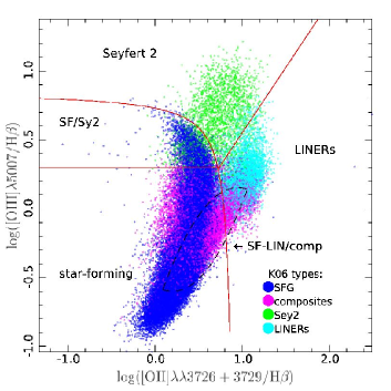
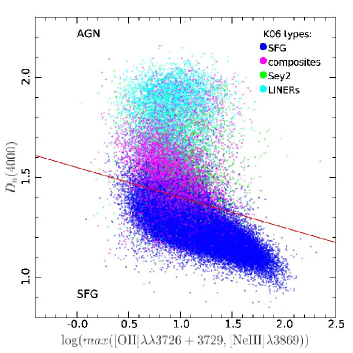
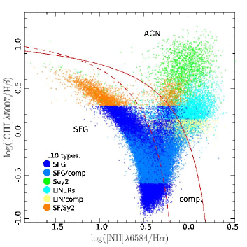
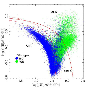
Figure 1: Summary of existing schemes for the classification of emission-line galaxies at high redshift. Top: results of the reference diagnostic (Kewley et al., 2006) are shown in the log$\left([\mathrm{O\textrm{{iii}}}]\lambda 5007/\mathrm{H}\beta\right)$ vs. the $\log\left([\mathrm{O}\textrm{{ii}}]\lambda\lambda 3726+3729/\mathrm{H}\beta\right)$ diagram (left) and in the $D_{n}(4000)$ vs. $\mathrm{max\left(EW[O\textsc{ii}],EW[Ne\textsc{iii}]\right)}$ diagram (right). The code is blue: SFG; green: Seyfert 2; cyan: LINERs; magenta: composites. Bottom: The results of the high-redshift classifications are shown in the standard log$\left([\mathrm{O\textrm{{iii}}}]\lambda 5007/\mathrm{H}\beta\right)$ vs. log$\left([\mathrm{N}\textsc{ii}]\lambda 6583/\mathrm{H}\alpha\right)$ diagram. Left: the L10 diagnostic (Lamareille, 2010). Right: the DEW diagnostic (Stasińska et al., 2006). Same color code as above except green: stands for all AGNs in the bottom-right panel; light blue: SFG/comp; yellow: LIN/comp; orange: SF/Sy2.In bottom-right panel, the long dashed line is the boundary between SFG and AGN used by Stasińska et al. (2006).

Figure 1 shows how the different types of galaxies (according to K06) appear in the high-redshift diagrams (top panels) and how the high redshift classifications appear back in one of the K06 diagnostic diagrams (bottom panels). In all panels, SFG are plotted in blue, Seyfert 2 in green (except in the bottom-right panel where green points stand for all types of AGNs), LINERs in cyan, and composites in magenta. The L10 diagnostic (left panels) implies several regions where different types of galaxies get mixed. Seyfert 2 region and LINERs region are now quite well defined, but we see composites falling in the SFGs and LINERs regions. Most of the composites fall in the region of the L10 diagnostic called SF-LIN/comp(marked by the dashed contour corresponding to Eqs. 7 and 8). SFGs and Seyfert 2 are now separated quite well, but still there is a small region of the L10 diagnostic, called SF/Sy2, where they get mixed. In the bottom-left panel, it seems that most of the SF/Sy2 galaxies belong to the K06 SFG region, and that a large number of SFG/comp galaxies belong to K06 SFG region. LIN/comp galaxies seem to appear half/half in the K06 composites and LINERs regions.

We now the compare K06 and DEW classifications (right panels). We see that all K06 LINERs are correctly classified as AGNs in the DEW diagnostic. Most of K06 Seyfert 2 galaxies lie in the DEW AGN region as well, so that is quite satisfying. However composites are shared in DEW SFG and AGN regions, which confirms that composites are sort of hybrids between AGNs and SFGs, also in terms of stellar populations. Thus they obviously cannot be isolated in the DEW diagnostic. We emphasize that the definition of SFG and AGN galaxies used in Stasińska et al. (2006) is slightly different from the K06 scheme: it is based on the long-dashed curve shown in the bottom-right panel of Fig. 1 (Eq. 11 of their paper). The DEW diagnostic is designed to exclude only pure SFGs without any AGN contribution, while according to Stasińska et al. (2006) galaxies classified as SFG by K06 (and by us) would allow up to 3% AGN contribution. Composites would allow up to 20% AGN contribution.

Indeed in the bottom-right panel, a non-negligible number of DEW AGNs actually belong to the K06 SFG or composite regions.However, we also note conversely that a non-negligible number of DEW SFGs contaminate the K06 composite and AGN regions. The DEW diagnostic actually fails to completely exclude all pure SFGs.

4 Limits of the L10 and DEW classifications

4.1 Success and contamination charts

Table 1: Success chart of the L10 diagnostic, where numbers are the probability that a given reference K06 type goes in a given L10 type.

^∗ union of SFG/Sy2, SFG, and SFG/comp regions.

^∗∗ union of the LINERs and LIN/comp regions.

Table 2: Contamination chart for the L10 diagnostic, where numbers are the probability that a given L10 type actually is any of the reference K06 types.

^∗ union of SFG/Sy2, SFG, and SFG/comp regions.

^∗∗ union of the LINERs and LIN/comp regions.

The success chart consists in classifying galaxies from our sample according to the reference, then associating a probability for each type of galaxy (AGN, composite, or SFG) to be classified correctly in the new diagnostic. The contamination chart is based on the same principle as the success chart, except this time we classify galaxies according to the new diagnostic, and then we calculate the probability that the galaxies classified as one type are actually of that same type according to the reference. Table 1 shows the success chart of the L10 diagnostic. It reveals a relatively satisfying spread of composite galaxies and AGNs inside the different types defined. Table 2 shows the associated contamination chart. We notice quite good efficiency, i.e. low contamination by other types, in the L10 SFG, Seyfert 2, and LINER regions.

If we take a look at AGNs, we notice that almost 60% of K06 Seyfert 2 galaxies are successfully classified as L10 Seyfert 2. Moreover 26% belong to the L10 SFG/Sy2 region, which would give us a total of more than 85% of K06 Seyfert 2 galaxies being classified as Seyfert2 with the L10 diagnostic. However, the contamination chart shows that the L10 SFG/Sy2 region is actually made up of only 21% K06 Seyfert 2, which means it cannot be used to reliably look for additional Seyfert 2 galaxies in high-redshift samples. The Seyfert 2 region itself shows a very low contamination (13%) by other types.

Most K06 LINERs (74%) are also successfully classified as L10 LINERs, and 17% belong to the L10 LIN/comp region. That gives a global success rate of 91% for LINERs. As already stated in Paper I, these results are much better than results produced by the former L04 diagnostic; however, the contamination by composites in the LIN/comp region is not negligible. Only 40% of the L10 LIN/comp objects actually are K06 LINERs, and 57% are K06 composites. That gives a global 37% contamination in the union of the L10 LINERs and LIN/comp regions.

Finally we confirm the conclusion of Paper I from these two tables, which is that the L10 diagnostic is very efficient for SFGs. If we consider the union of the L10 SFG, SFG/Sy2, and SFG/comp regions, the success rate is 99.7% and the contamination by other types only 16%. This low contamination by composite galaxies and AGNs, in particular in the SFG/Sy2 and SFG/comp regions, has been shown to not critically bias SFG studies such as metallicity. Lamareille et al. (2009), for instance, performed such tests using the L04 diagnostic, i.e. with an even more contamination by AGNs in the SFG region.

Table 3: Success chart for DEW diagnostic

Table 4: Contamination chart for DEW diagnostic

Tables 3 and 4 show the success and contamination charts of the DEW diagnostic. Again, the results are very good for SFGs with a 95% success rate, and only an 8% contamination, less than for L10. Still, this better contamination chart for SFGs does not drastically reflect a worse success rate for AGNs. The success rate is indeed 80% for Seyfert 2 and 98% for LINERs. The DEW has in fact greater ability to separate SFGs from AGNs than standard diagnostic diagrams as in K06 or L10 classifications. However, the main limitations of the DEW diagnostic clearly appear from the contamination chart regarding DEW AGNs. The DEW AGN region is actually made up of only 37% K06 AGNs. There is indeed a high contamination by 18% K06 SFGs, much higher than with the L10 diagnostic (less than 3% in the Seyfert 2 and LINERs regions). Moreover, the DEW AGN region is contaminated by 45% K06 composites, to be compared to 30% for the L10 LINERs, and only 1% for the L10 Seyfert 2. As one can see in Fig. 1, composites get completely confused with Seyfert 2 and LINERs in the DEW diagnostic, while they are rather confused with SFGs in the L10 diagnostic. We do note that this contamination is explained mainly by the fact that Stasińska et al. (2006) use a different definition of SFGs and AGN galaxies (as discussed in Sect. 3.4 above). Indeed, in DEW diagnostic’s philosophy, it should not be considered as a “contamination” but as a “contribution” of an AGN to star-forming galaxies. Finally, the DEW diagnostic does not allow any distinction between Seyfert 2 and LINERs.

Regarding the classification of SFGs, we conclude that one should use the L10 diagnostic for its very high success rate and DEW diagnostic for its lower contamination. About AGNs, both advantages of the L10 and DEW diagnostic diagrams may be put together to provide a better diagnostic, which is the goal of the present paper. We emphasize that we did not use the DEW diagnostic itself for our own classification. We only used the DEW diagram to derive a new diagnostic where it is needed (see Sect. 4.2 below).

4.2 AGN counts

In order to explore the limitations of L10 and DEW classifications of AGNs better, we now count the number of AGNs (Seyfert 2 and LINERs) as a function of the ionization state, roughly given by the $\log\left([\mathrm{O}\textsc{iii}]/\mathrm{H}\beta\right)$ emission-line ratio. To achieve this test, we divide the K06 or L10 diagnostic diagrams in equal horizontal slices, and then in each slice we count the number of AGNs. Figure 2 shows the absolute and difference counts (relative to K06) obtained with, from left to right, the following classifications: L04, DEW, L10, and the present paper’s diagnostic (see Sect. 5 below). In each panel, the results are compared to the actual count of AGNs according to the reference K06 diagnostic.

We confirm, as stated in Paper I, that the L04 diagnostic tends to underestimate the amount of AGNs, even when including L04 candidate AGNs, and that a very high number of AGNs (mainly LINERs) are lost in this diagnostic. However, we can put this effect into context thanks to Fig. 2, as we see that it only becomes significant for $\log\left([\mathrm{O}\textsc{iii}]/\mathrm{H}\beta\right)\lesssim 0.9$, or $\log\left([\mathrm{O}\textsc{iii}]/\mathrm{H}\beta\right)\lesssim 0.7$ if we include candidate AGNs. For AGNs with a high ionization state, the L04 diagnostic indeed gives perfect results.

Figure 2 also shows that DEW and L10 classifications are doing quite well by following the K06’s curve almost exactly for $\log\left([\mathrm{O}\textsc{iii}]/\mathrm{H}\beta\right)\gtrsim 0.25$. In both cases, we notice an underestimate of the number of AGNs for $0.25\lesssim\log\left([\mathrm{O}\textsc{iii}]/\mathrm{H}\beta\right)\lesssim 0.7$, where this effect is more significant for the L10 diagnostic than for the DEW diagnostic. Nevertheless, the DEW diagnostic clearly overestimates the number of AGNs in low ionization states, i.e. mainly LINERs ($\log\left([\mathrm{O}\textsc{iii}]/\mathrm{H}\beta\right)\lesssim 0.25$). In this region, the L10 diagnostic, in contrast, satisfyingly follows the K06’s curve, with a small underestimate.

Unfortunately, including the SFG/Sy2 and LIN/comp regions does not help. It makes a peak of galaxies at $\log\left([\mathrm{O}\textsc{iii}]/\mathrm{H}\beta\right)\simeq 0.4$ appear that does not fit the reference profile, while in a lower ionization state the number of AGNs is now clearly overestimated. Those two effects are from the high contamination of the L10 SFG/Sy2 region by K06 SFGs and of the L10 LIN/comp region by K06 composites.

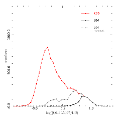
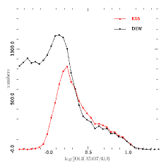
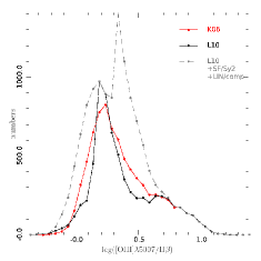
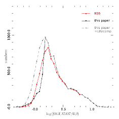
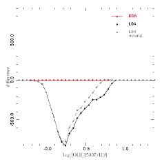
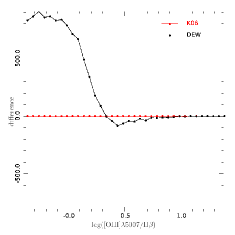
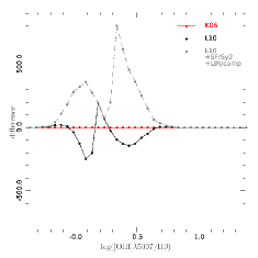
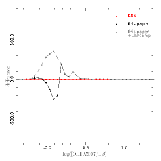
Figure 2: Comparison between the number of AGNs (Seyfert 2 and LINERs) counted with different calibrations at high redshift, as a function of log$\left([\mathrm{O\textrm{{iii}}}]\lambda 5007/\mathrm{H}\beta\right)$. From left to right, the calibrations used are L04, DEW, L10 (paper I), and the present paper. Top panels show absolute counts. Bottom panels show difference counts. In each panel, the reference counts established with the K06 diagnostic are shown in red, and the counts obtained with the high-redshift diagnostic are shown in black. The gray dashed lines show the results when including “candidate” regions, i.e. for L04, L10, and the present paper’s classifications: candidate AGNs region; SFG/Sy2 and LIN/comp regions; LIN/comp region.

5 The supplementary M11 diagnostic

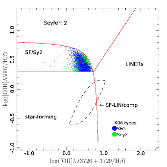
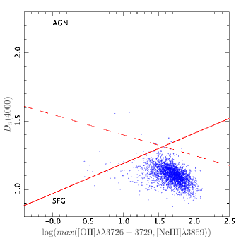
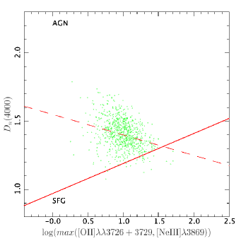
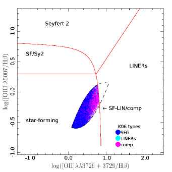
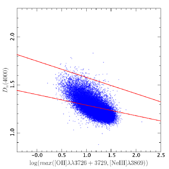
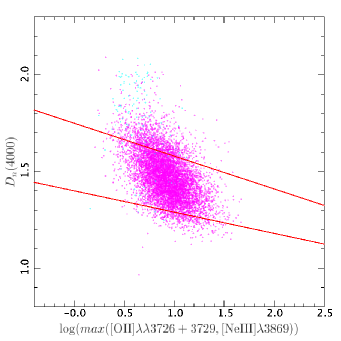
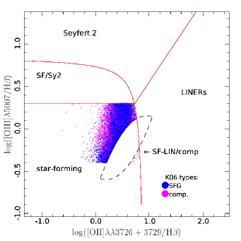
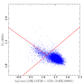
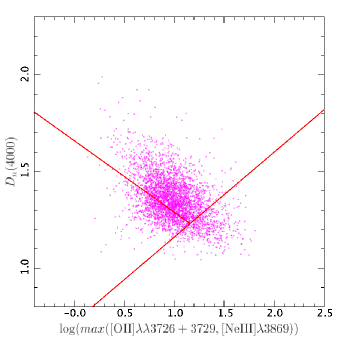
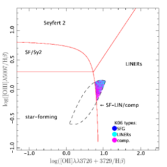
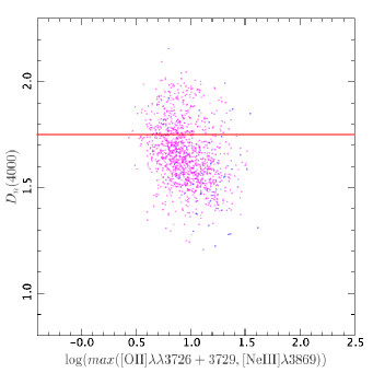
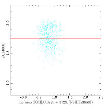
Figure 3: Left: In the $\log\left([\mathrm{O}\textsc{iii}]\lambda 5007/\mathrm{H}\beta\right)$ vs. $\log\left([\mathrm{O}\textrm{{ii}}]\lambda\lambda 3726+3729/\mathrm{H}\beta\right)$ diagram, the different regions where galaxies of different types are mixed (color-code according to the reference K06 diagnostic). The curves are the ones from the Lamareille (2010) diagnostic. Center and right: The same points as in the associated left panels, but now in the $D_{n}(4000)$ vs. $\mathrm{max\left(EW[O\textsc{ii}],EW[Ne\textsc{iii}]\right)}$ diagram. For clarity, we plot the different types in two panels.The solid lines show the adopted demarcation lines (see text for details). The dashed line in top-right panels is the separation adopted by Stasińska et al. (2006).

Figure 3 shows four regions where galaxies of different types (according to the reference K06diagnostic) are confused in the $\log\left([\mathrm{O}\textsc{iii}]\lambda 5007/\mathrm{H}\beta\right)$ vs. $\log\left([\mathrm{O}\textrm{{ii}}]\lambda\lambda 3726+3729/\mathrm{H}\beta\right)$ diagram. It shows also in its center and right panels how these galaxies behave in the $D_{n}(4000)$ vs. $\mathrm{max\left(EW[O\textsc{ii}],EW[Ne\textsc{iii}]\right)}$ diagram. From top to bottom, the four studied regions are SFG/Sy2, SFG/comp, another SFG/comp region not defined in the L10 diagnostic but where a non negligible number of the composites (25%) are still mixed with SFGs, and LIN/comp.

5.1 The SFG/Sy2 region

In the L10 SFG/Sy2 region (see Fig. 3 top), K06 Seyfert 2 and SFGs are confused. It is unfortunately obvious in the bottom-left panel that the DEW diagnostic does not separate the two classes of objects correctly in the L10 SFG/Sy2 region. We thus propose a new demarcation line to separate K06 Seyfert 2 from SFGs, valid only in the L10 SFG/Sy2 region, with the equation

$$D_{n}(4000)=0.22\times\mathrm{\log\left(max\left(EW[O\textsc{ii}],EW[Ne\textsc{iii}]\right)\right)}+0.97.$$ (10)

Seyfert 2 would fall above this line, SFG below.The slope and zero point of this line have been optimized by minimizing on a grid the following function:

$$\chi^{2}=(1-S^{A})^{2}+(1-S_{B})^{2}+(C^{A})^{2}+(C_{B})^{2},$$ (11)

where $S^{A}$, $S_{B}$, $C^{A}$, $C_{B}$ are the success rate for AGN above the defined line, the success rate for SFG below the line, the contamination by SFG above the line, and the contamination by AGN below the line (all values between 0 and 1), respectively. Indeed, we want to maximize the success rates and minimize the contamination at the same time above and below the defined line. The grid is done in $0.01$dex steps in both slope and zero point. To minimize computer time, limits on this grid are defined by eye.

Table 5: Success chart for the supplementary M11 diagnostic in the L10 SFG/Sy2 region.

	reference K06
M11	SFG	Seyfert 2
total	100	100
SFG	99.10	3.10
Seyfert 2	0.90	96.90

We have established the success of our new diagnostic in the L10 SFG/Sy2 region (see Table 5). This chart shows that our demarcation line works almost perfectly and can be used in that area. We have now correctly classified almost all actual Seyfert 2 in our sample: 97% of those in the L10 SFG/Sy2 region are classified as Seyfert 2. Given that 59% of the K06 Seyfert 2 in the whole sample were already correctly classified, and 26% of them classified as L10 SFG/Sy2, this increases the global success rate to 85%. This is the best success rate one can obtain by combining L10 and DEW diagrams. The contamination in the SFG/Sy2 region is made of 3.1% SFGs above the line defined by Eq. 10 and 0.9% Seyfert 2 below it.

5.2 The SFG/comp region

The L10 SF/comp (see Fig. 3 second line) contain composites, SFGs, and very few LINERs. Following the optimization procedure explained above, we find the following equation which separate as many SFGs as possible from composites:

$$D_{n}(4000)=-0.11\times\mathrm{\log\left(max\left(EW[O\textsc{ii}],EW[Ne\textsc{iii}]\right)\right)}+1.4,$$ (12)

where SFGs are below this line. Since SFGs dominate the sample, the region below this line is composed of 98% SFGs. Conversely, the region above this line is still a mix between SFGs (59%), composites (36%), and a few LINERs (4%). We again applied the optimization procedure but now only consider the latest region, in order to isolate pure composites as much as possible. We obtain:

$$D_{n}(4000)=-0.17\times\mathrm{\log\left(max\left(EW[O\textsc{ii}],EW[Ne\textsc{iii}]\right)\right)}+1.75,$$ (13)

where composites are above the line, SFG/comp below it (i.e. between the two lines).

Table 6: Success chart for the supplementary M11 diagnostic in the L10 SFG/comp region.

	reference K06
M11	SFG	LINERs	composites
total	100	100	100
SFG	63.69	3.47	5.31
composites	0.19	70.14	13.95
SFG/comp	36.12	26.39	80.74

Table 7: Contamination chart for the supplementary M11 diagnostic in the L10 SFG/comp region.

	reference K06
M11	total	SFG	LINERs	composites
SFG	100	98.30	0.02	1.67
composites	100	5.85	8.21	85.93
SFG/comp	100	68.81	0.19	31.00

Tables 6 and 7show the success chart and the contamination chart of the supplementary M11 diagnostic, in the L10 SFG/comp region. From all the K06 SFGs present in this region, 64% are now correctly classified as SFGs, another 36% being still ambiguously classified as SFG/comp.It is unfortunately impossible to increase this success rate without misclassifying too many K06 composites as SFGs. Only 14% of K06 composites could be isolated. Newly isolated SFGs are not significantly contaminated by K06 composites (2%), and neither are the newly isolated composites by K06 SFGs (6%). The majority of the K06 of composites (81%) are still ambiguously classified as SFG/comp. The best reason to use this diagram is clearly for isolating SFGs. The SFG/comp region is now made of 69% K06 SFGs and 31% K06 composites, which is more balanced than in Paper I (respectively 83% and 17%).

5.3 Additional region of composites mixed with SFGs

We define a last region where K06 composites are mixed with K06 SFGs in the L10 diagnostic. It is located below the SFG/Sy2 region, and above $\log\left([\mathrm{O}\textsc{iii}]\lambda 5007/\mathrm{H}\beta\right)>-0.4$, excluding the SFG/comp region (see Fig. 3 third line). Even though we can see that these K06 SFGs are mostly spread over the bottom right of the DEW diagnostic diagram and K06 composites are slightly above, there is still a small area where they get together.

Following the same optimization procedure as above, we first fit the optimized demarcation line between pure SFGs and SFGs mixed with composites:

$$D_{n}(4000)=0.44\times\mathrm{\log\left(max\left(EW[O\textsc{ii}],EW[Ne\textsc{iii}]\right)\right)}+0.72,$$ (14)

where SFGs are below this line. As in previous section, the region above this line contains a mix of SFGs (25%) and composites (75%). In this region, we fit another optimized demarcation line between pure composites and composites mixed with SFGs:

$$D_{n}(4000)=-0.37\times\mathrm{\log\left(max\left(EW[O\textsc{ii}],EW[Ne\textsc{iii}]\right)\right)}+1.66,$$ (15)

where composites are above this line, and SFG/comp below it (i.e. between the two lines). We finally add the remaining mixed galaxies to the SFG/comp type.

Table 8: Success chart for the supplementary M11 diagnostic in the additional region of the L10 diagnostic where SFG are mixed with composites.

	reference K06
M11	SFG	composites
total	100	100
SFG	92.10	12.69
composites	2.90	61.97
SFG/comp	5.00	25.34

Table 9: Contamination chart for the supplementary M11 diagnostic in the additional region of the L10 diagnostic where SFG are mixed with composites.

	reference K06
M11	total	SFG	composites
SFG	100	96.39	3.61
composites	100	14.50	85.30
SFG/comp	100	42.08	57.92

Tables 6 and 9 show the success and contamination charts of the supplementary M11 diagnostic in this last region. Of all K06 SFGs present in this region, 92% are now correctly classified, and another 5% are ambiguously classified as SFG/comp. We also managed to isolate 62% of the K06 composites falling in this region, which is an improvement compared to the L10 diagnostic. Conversely, 12% of the K06 composites are now unfortunately misclassified as SFGs. This is still an improvement : we recall that 100% of the K06 composites in this region used to be classified as SFGs with the L10 diagnostic. Most of them (62%) are now classified as composite galaxies, and another 25% are still ambiguously classified as SFG/comp. The composites defined in this region are contaminated by 15% K06 SFGs, which may not be neglected. The SFG/comp galaxies defined in this region are made of approximately half K06 SFGs (42%) and half K06 composites (58%).

5.4 The LIN/comp region

Figure 3 (bottom) shows the LIN/comp region of the L10 diagnostic in the DEW diagnostic diagram. It is clear that this diagram cannot be used to isolate LINERs cleanly from composites. Indeed, one may argue that LINERs are more concentrated on the top and composites on the bottom of the diagram, so we propose a straight line at $D_{n}(4000)\approx 1.75$ as a separation. Using this line we find, however, 61% LINERs and 39% composites above, 28% and 72% below respectively, which is unsatisfactory. Thus, we do not update the LIN/comp region as in Paper I.

5.5 Discussion

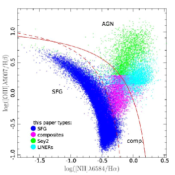
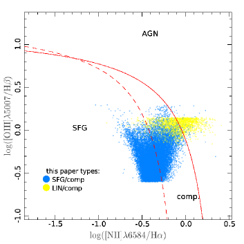
Figure 4: Results of the new diagnostic derived in the present paper in the standard log$\left([\mathrm{O\textrm{{iii}}}]\lambda 5007/\mathrm{H}\beta\right)$ vs. log$\left([\mathrm{N}\textsc{ii}]\lambda 6583/\mathrm{H}\alpha\right)$ diagram. For clarity, only SFGs, AGNs and composites are shown in the left panel, while SFG/comp and LIN/comp are shown in the right panel. Same color code as in Fig. 1.

Figure 4 shows our supplementary M11 diagnostic combined with L10 diagnostic, in one of the standard K06 diagnostic diagrams. The left panel looks pretty good: SFGs Seyfert 2, LINERs, and some composites lie almost perfectly in the correct corresponding regions of this diagram. In contrast, the right hand panel shows the limitations: objects that are still ambiguously classified or as SFG/comp or as LIN/comp. Anyway, comparing Fig. 4 to the bottom left hand panel of Fig. 1, we see a clear improvement.

Table 10: Overall success chart for the L10 and M11 diagnostics.

	reference K06
L10/M11	SFG	Composites	Seyfert 2	LINERs
total	100	100	100	100
SFG	77.97	8.92	0.92	0.10
SFG/comp	20.99	50.97	0.47	0.98
composites	0.66	23.44	5.46	4.30
Seyfert 2	0.12	0.93	84.71	3.93
LINERs	0.17	6.94	8.00	73.51
LIN/comp	0.11	8.81	0.44	17.18
total SFG1	98.96	59.88	1.39	1.08
total LINERs2	0.27	15.74	8.44	90.70
total comp.3	21.75	83.22	6.38	22.46

¹ SFG+SFG/com

² LINERs+LIN/comp

³ composites+SFG/comp+LIN/comp.

Table 11: Overall contamination chart for the L10 and M11 diagnostics.

	reference K06
L10/M11	total	SFG	Composites	Seyfert 2	LINERs
SFG	100	97.68	2.26	0.05	0.01
SFG/comp	100	66.81	32.89	0.07	0.23
composites	100	11.02	79.77	3.99	5.23
Seyfert 2	100	2.73	4.42	86.20	6.66
LINERs	100	2.28	19.40	4.80	73.51
LIN/comp	100	3.37	56.57	0.61	39.46
total SFG1	100	75.83	15.37	3.30	5.50
total LINERs2	100	2.61	30.68	3.53	63.18
total comp.3	100	53.67	41.63	0.68	4.02

¹ SFG+SFG/com

² LINERs+LIN/comp

³ composites+SFG/comp+LIN/comp.

Tables 10 and 11 establish new contamination and success charts in order to get a more precise measurement of this improvement. Success chart shows that 1% of K06 SFG are classified in a region where they are not supposed to be. K06 composites are predominantly found in the SFG/comp region (51%) than in the composite region (23%). This is an improvement over Paper I, but it shows that neither the L10 nor the DEW diagrams are really good at identifying composites at high redshift. K06 Seyfert 2 galaxies and LINERs have a high success rate (respectively 85% and 74%), which is for Seyfert 2 galaxies a really good improvement compared to Paper I. For K06 LINERs, the success rate increases to 91% including the LIN/comp, but one has to be aware that this region is actually made of only 39% K06 LINERs and is dominated by 57% K06 composites.

Nevertheless, one can conclude from the contamination chart that SFGs, Seyfert 2, and LINERs are not significantly contaminating each other. The main contamination comes in all cases from composites: 33% in the SFG/comp region, 19% in the LINERs region, and 57% in the LIN/comp region. It is conversely very low in the SFG and Seyfert 2 regions.

One could worry about aperture effects. Indeed, SDSS spectra are based on 3” fibers. This may end in overestimated $D_{n}(4000)$ values for close objects where only the central bulge is covered by the fiber. However, one can see in Fig. 3 that only objects with $D_{n}(4000)<1.5$ could change their classification with a significant aperture effect. Looking at Fig. 16 in Kauffmann et al. (2003b), we see that those objects do not actually suffer from a strong aperture effect. We conclude that our diagnostic is not biased by this effect.

Finally, we invite the reader to take a look at the right hand panels of Fig. 2. It shows the AGN counts obtained with our new supplementary M11 diagnostic combined with L10 diagnostic. We clearly see that the diagnostic derived in the present paper is the one that follows the reference K06 curve more accurately. There are still problems for $\log\left([\mathrm{O}\textsc{iii}]/\mathrm{H}\beta\right)\lesssim 0.25$, which is normal since we did not manage to change the classification of LINERs by adding the DEW diagnostic diagram.

6 Conclusion

By adding the M11 diagnostic to the L10 diagnostic derived in Paper I, we now have a very good classification of emission-line galaxies that can be used on high-redshifts samples. The main improvements compared to Paper I are

• The unambiguous classification of objects in the former SFG/Sy2 region as SFGs or Seyfert 2.

• The unambiguous classification of some of the objects in the SFG/comp region as SFGs or composites (where no composites at all were found in Paper I).

• A better definition of the SFG/comp region, which leaves fewer possible composites not flagged as such. We emphasize again that this region is in any case dominated by SFGs.

No improvements could have been done in the LIN/comp region, which is left unchanged compared to Paper I.

In order to use the diagnostic derived in this paper, one should follow these steps.

1. Classify objects in the $\log\left([\mathrm{O}\textsc{iii}]\lambda 5007/\mathrm{H}\beta\right)$ vs. $\log\left([\mathrm{O}\textrm{{ii}}]\lambda\lambda 3726+3729/\mathrm{H}\beta\right)$ with the L10 diagnostic derived in Paper I (see also equations in Sect. 3.2).

2. Classify objects falling in the SFG/Sy2 region as SFGs or Seyfert 2 using Eq. 10.

3. Isolate objects falling the the SFG/comp region as

   1. SFGs using Eq. 12, and

   2. composites using Eq. 13.

4. Define a new SFG/comp region inside the SFG region using $\log\left([\mathrm{O}\textsc{iii}]\lambda 5007/\mathrm{H}\beta\right)>-0.4$, so inside this new region, isolate

   1. SFGs using Eq. 14, and

   2. composites using Eq. 15.

In both points (3) and (4) above, objects not classified as SFGs or composites remain of the ambiguous SFG/comp type. We invite the reader to look at the “JClassif” software (available at: http://www.ast.obs-mip.fr/galaxie/), which performs these steps automatically on any sample, as well as other classification schemes.

Table 11 may be used as a probability chart showing whether each type in our diagnostic is one of the K06 reference types. However, we warn the reader that the relative proportions of SFGs, composites and AGNs in each regions of our diagnostic diagrams may evolve with redshift compared to the SDSS sample. Finally, we note that it is possible to upgrade this classification to higher redshifts where $[\mathrm{O}\textsc{iii}]\lambda 5007$ and $\mathrm{H}\beta$ emission lines get red-shifted out of the spectra ($1.0\apprle z\apprle 1.5$ on optical spectra). To that goal one may use the equations provided by Pérez-Montero et al. (2007), which convert $[\mathrm{Ne}\textsc{iii}]\lambda 3869$ and $\mathrm{H}\delta$ to $[\mathrm{O}\textsc{iii}]\lambda 5007$ and $\mathrm{H}\beta$.