Implicitization of surfaces via geometric tropicalization

Abstract.

In this paper we further develop the theory of geometric tropicalization due to Hacking, Keel and Tevelev and we describe tropical methods for implicitization of surfaces. More precisely, we enrich this theory with a combinatorial formula for tropical multiplicities of regular points in arbitrary dimension and we prove a conjecture of Sturmfels and Tevelev regarding sufficient combinatorial conditions to compute tropical varieties via geometric tropicalization. Using these two results, we extend previous work of Sturmfels, Tevelev and Yu for tropical implicitization of generic surfaces, and we provide methods for approaching the non-generic cases.

1. Introduction

In its ten years of existence, the field of tropical geometry has provided new tools to approach questions in algebraic geometry. Among them, we can include classical elimination and implicitization problems [9, 18, 19, 20]. In the classical setting, we wish to recover the defining ideal of either the projection of a subvariety of an algebraic torus or of a parametric variety. In the tropical setting, we replace the defining ideal by a polyhedral object, namely, its tropicalization. Such methods are known as tropical elimination and tropical implicitization and have been used recently for computations going beyond the power of classical elimination tools, including multidimensional resultants and Gröbner bases. Successful applications of tropical implicitization techniques were presented in [6, 7].

Tropical geometry is a polyhedral version of classical algebraic geometry: we replace algebraic varieties over the torus $\mathbb{T}^{r}=(\mathbb{C}^{*})^{r}$ by weighted, balanced polyhedral fans. These objects preserve just enough data about the original varieties to remain meaningful (e.g. dimension, degree, etc.), while discarding much of their complexity. They are also known in the literature as Bieri-Groves sets [3]. We can compute them based on Gröbner theory or valuations, depending on how the classical varieties are presented. Gröbner techniques are better suited for algebraic descriptions, while valuations provide the right framework in the presence of geometric information, e.g. a polynomial parameterization. The newly develop theory of geometric tropicalization, introduced by Hacking, Keel and Tevelev [14, $\S 2$], fits into the latter.

The crux of geometric tropicalization is to read off the tropicalization of a smooth closed subvariety of a torus directly from the combinatorics of its boundary in suitable compactification. To do so, its boundary is required to have simple normal crossings (snc), that is, to behave locally like an arrangement of coordinate hyperplanes. More precisely, let $X\subset\mathbb{T}^{r}$ be the subvariety and pick a normal and $\mathbb{Q}$-factorial compactification $\overline{X}$ where $X$ is an open subvariety of $\overline{X}$ and its divisorial boundary $\partial\overline{X}=\overline{X}\smallsetminus X$ is a snc boundary. The combinatorial information of the tropical variety $\mathcal{T}X$ is encoded in an abstract simplicial complex, called the boundary complex $\Delta(\partial\overline{X})$, which resembles the one in [16]. After assigning coordinates to the vertices of this complex by means of divisorial valuations, and extending linearly on cells, we get a complex in the real span of the cocharacter lattice of $\mathbb{T}^{n}$. Geometric tropicalization says precisely that the support of the tropical fan is the cone over this complex and, in particular, the result does not depend on our choice of $\overline{X}$ (Theorem 2.4).

The circle of ideas behind geometric tropicalization has deep, yet not explicit, connections to recent articles on tropical algebraic geometry. As an example, we can mention the work of M. Baker relating linear systems on curves and linear systems on the dual graphs of their associated semistable regular models [2]. These dual graphs encode the same combinatorial information as the boundary complexes used in [14, $\S 2$]. One possible explanation for this phenomenon is that, up to now, geometric tropicalization was only able to recover the support of the tropical fan. Tropical multiplicities were missing from this description and they are essential for recovering information about the original algebraic varieties from their tropical counterparts. By decoration the boundary complex $\Delta(\partial\overline{X})$ with weight on its maximal cells, we obtain an explicit combinatorial formula for computing tropical multiplicities (Theorem 2.5), complementing the set-theoretic results of [14, $\S 2$].

As one main expect, the major difficulty in applying these methods to compute tropical fans in concrete examples lies in the restrictive assumptions on the compactification $\overline{X}$. One way of constructing such an object is provided by a strong resolution of $X$ in the sense of Hironaka [15, Theorem 3.27]. These resolutions are by no means explicit, explaining the lack of examples in this theory. The algorithmic difficulties of performing such a task are numerous and it would be desirable to attenuated the necessary conditions on $\overline{X}$ to obtain $\mathcal{T}X$ from the weighted complex $\Delta(\partial\overline{X})$. After studying in detail the surface case, Sturmfels and Tevelev conjectured that the right condition to impose was not geometric but combinatorial, requiring the boundary components to intersect in the expected codimension [18]. They called it the combinatorial normal crossing (cnc) boundary condition. This property ensures that $\Delta(\partial\overline{X})$ is simplicial and has the right dimension, namely, one less than the dimension of $X$. In this paper, we prove this conjecture in arbitrary dimension, addressing the question of tropical multiplicities as well. Here is the precise statement, which we discuss in Section 2 (Theorem 2.8).

Theorem.

Let $X\subset\mathbb{T}^{n}$ be a smooth subvariety and let $\overline{X}$ be a normal and $\mathbb{Q}$-factorial compactification with combinatorial normal crossing boundary $\partial\overline{X}$. Then, the weighted set $\mathcal{T}X$ can be computed from $\overline{X}$ using the weighted boundary complex $\Delta(\partial\overline{X})$ and the divisorial valuations induced by $\partial\overline{X}$.

Tropical implicitization was pioneered by the work of Sturmfels, Tevelev and Yu [19]. Their methods are well suited for generic varieties, and are built on the theory of geometric tropicalization and the construction of tropical compactifications in the sense of Tevelev [21]. However, real life is seldom generic, so it is crucial to attack the non-generic versions of these problems. One of the contributions of this paper is to identify the genericity conditions, describe certificates for them, and introduce tropical implicitization methods for non-generic surfaces.

In Section 4 we focus our attention on the generic setting: surfaces parameterized by Laurent polynomial maps with fixed support and where we allow the coefficients to vary generically. Following [19], we translate our tropical implicitization question to the one of compactifying an arrangement of plane curves in the torus $\mathbb{T}^{2}$. These curves are precisely the vanishing locus of each coordinate of the given polynomial parameterization. The genericity conditions in [19] are chosen so that we have a natural choice for our cnc compactification: a smooth projective toric surface build from the supports of our parameterization. Our approach allows to weaken these conditions and still be able to compute our tropical surface from the input map. As a byproduct, in Theorem 4.1 we show that the smoothness condition on the ambient space is unnecessary to obtain the tropical surface encoded as a weighted graph. We illustrate our approach with several numerical examples in $\mathbb{C}^{3}$. These examples are then revisited to highlight the differences between the techniques applied to generic and non-generic surfaces.

In Section 5 we discuss tropical implicitization of non-generic surfaces. We start by clarifying what we mean by special surfaces. Then, we describe a procedure to obtain the graphs associated to their tropicalization. Singularities coming from excessive intersections are the main obstruction to apply the methods of Section 4 in this context. To fix this bad behavior, we first compactify the arrangement of plane curves inside $\mathbb{P}^{2}$. Secondly, since the cnc condition on the boundary fails to hold, we must resolve the excessive boundary points, for example, by ordinary blow-ups. This construction yields the desired cnc compactification. Thus, the corresponding tropical surface can be obtained using Theorem 2.8.

We end this paper with some remarks and open questions. As our running examples illustrate, rational surfaces in $\mathbb{C}^{3}$ serve as a nice test case to explore tropical implicitization techniques. In this setting, these methods require to analyze the combinatorics of a curve arrangement in $\mathbb{T}^{2}$, and the local behavior at points belonging to three or more of these curves. Topological methods from singularity theory can then be applied to predict the resulting tropical surfaces. Even though the theory of tropical implicitization is at an early stage and it is still evolving, we expect Theorems 2.5 and 2.8 to become a valuable tool for future applications.

2. Geometric tropicalization

In this section, we discuss the theory of geometric tropicalization. We present its original formulation in set-theoretic terms as in [14], and we extend it with two results. The first main result is a formula for tropical multiplicities. The second one proves a conjecture of Sturmfels and Tevelev [18] on necessary conditions to compute tropical varieties from their boundary complexes and their associated divisorial valuations. More precisely, rather than requiring a simple normal crossing (snc) boundary, it is enough to require a combinatorial normal crossing (cnc) boundary. The main advantage of this weaker hypothesis will become evident in Sections 4 and 5.

Notation 2.1.

Throughout this paper, we fix the following notation. Let $\mathbb{T}^{r}$ be the $r$-dimensional algebraic torus over a field $k$ of characteristic zero. Let $\Lambda_{r}=\operatorname{Hom}(k^{*},\mathbb{T}^{r})$ be the cocharacter lattice and $\Lambda_{r}^{\vee}=\operatorname{Hom}(\mathbb{T}^{r},k^{*})$ the character lattice. We let $K|k$ be the field of Puiseux series with parameter $\varepsilon$ and with valuation

$$\mathbf{\operatorname{ord}}\colon K\to\mathbb{R}\cup\{\infty\},\qquad\alpha\,\varepsilon^{u}+(\text{higher order terms})\mapsto u.$$

Given a fan $\mathcal{F}$ in $\mathbb{R}\otimes\Lambda_{r}$ we let $X_{\mathcal{F}}$ be the associated toric variety, with intrinsic torus $\mathbb{T}^{r}$. As it is standard in toric geometry, given a cone $\Sigma$ of $\mathcal{F}$, we let $V(\Sigma)\subset X_{\mathcal{F}}$ be the closure of the torus orbit $\mathcal{O}_{\Sigma}$, with intrinsic torus $\mathbb{T}_{\Sigma}$.

We start by recalling the basics on tropical geometry [4]. Our exposition will be coordinate free, but the reader can safely pick a basis of characters for each $r$-dimensional algebraic tori and view all tropical varieties in $\mathbb{R}^{r}$ rather than in the $\mathbb{R}$-span of the cocharacter lattice.

The tropicalization of a closed subvariety $X$ of the algebraic torus $\mathbb{T}^{r}$ is a fan in $\mathbb{R}\otimes\Lambda_{r}$ with intrinsic lattice $\Lambda_{r}$. It is defined as:

(1) $$\mathcal{T}X=\{w\in\Lambda_{r}\mid 1\notin\operatorname{in}_{w}(I_{X})\}.$$

Here, $I_{X}$ is the defining ideal of $X$ in the Laurent polynomial ring $k[\Lambda^{\vee}_{r}]$, and $\operatorname{in}_{w}(I_{X})$ is the ideal of all initial forms $\operatorname{in}_{w}(f)$ for $f\in I_{X}$. The set $\mathcal{T}X$ is a rational polyhedral fan of dimension $\dim X$ [3]. A point $w\in\mathcal{T}X$ is called regular if there exists a vector subspace $\mathbb{L}_{w}\subset\mathbb{R}\otimes\Lambda_{r}$ such that $\mathcal{T}X$ and $\mathbb{L}_{w}$ agree locally near $w$. The tropical variety $\mathcal{T}X$ can be endowed with a locally constant function called multiplicity, defined on regular points, and that satisfies a balancing condition [18, Definition 3.3]. There are many ways of defining these numbers. For example, $m_{w}$ can be computed as the sum of the multiplicities of all minimal associated primes of the initial ideal $\operatorname{in}_{w}(I_{X})$ [9, $\S 2$]. Similarly, if $\Sigma$ is a cone in $\mathcal{T}X$ that contains $w$ we can define $m_{w}$ as the length of the 0-dimensional scheme $V({\Sigma})\cap Z$, where $Z$ is the closure of $X$ in the toric variety associated to the fan $\mathcal{T}X$ [18, Lemma 3.2]. Theorem 2.5 gives an alternative combinatorial approach for obtaining these invariants.

The theory of geometric tropicalization aims to compute tropical varieties from geometric information on the underlying classical varieties. Our main players are the notions of cnc and snc pairs, and their associated boundary complex. Roughly speaking, starting from a smooth closed subvariety $X\subset\mathbb{T}^{r}$ we find a cnc pair $(\overline{X},\partial\overline{X})$ and we construct a quotient of the boundary complex $\Delta(\partial\overline{X})$ from [16]. This simplicial complex collects the combinatorial structure of the tropical fan $\mathcal{T}X$. Here are the precise definitions:

Definition 2.2.

Let $X$ be a smooth subvariety of a torus $\mathbb{T}^{r}$, and let $\overline{X}$ be a normal and $\mathbb{Q}$-factorial compactification containing $X$ as a dense open subvariety. Let $\partial\overline{X}=\overline{X}\smallsetminus X$ be the boundary divisor of $\overline{X}$. We say that this boundary is a combinatorial normal crossings divisor if for every integer $l$, and any choice of $l$ boundary components, their intersection has codimension $l$. Similarly, the boundary is a simple normal crossings divisor if, in addition, this intersection is transverse (i.e. the intersection behaves locally like a hyperplane arrangement). We say that $(\overline{X},\partial\overline{X})$ is a combinatorial normal crossing pair or cnc pair for short, if the boundary is a combinatorial normal crossing divisor. Simple normal crossing pairs (snc pairs for short) are defined analogously.

Note that the normality condition on $\overline{X}$ is imposed so that we can define the order of vanishing of a rational function along an irreducible divisor. The $\mathbb{Q}$-factorial property says that Weil divisors are $\mathbb{Q}$-Cartier and it enables us to view Cartier divisors as a subgroup all Weil divisors, thus, allowing us to speak of divisors without further distinction. In addition, in this setting, intersection numbers among boundary components are well defined [13, Chapter 2]. These numbers will be crucial when discussing tropical multiplicities. If $\overline{X}$ is smooth, then the normality and $\mathbb{Q}$-factorial conditions are automatically achieved. In the language of [21], cnc pairs will yield tropical compactifications of subvarieties of tori.

Definition 2.3.

Let $(\overline{X},\partial\overline{X})$ be a cnc pair. The boundary complex $\Delta(\partial\overline{X})$ is a simplicial complex whose vertices $\{v_{1},\ldots,v_{m}\}$ are in one-to-one correspondence with the $m$ components of the boundary divisor $\partial\overline{X}=\bigcup_{i=1}^{m}D_{i}$. Given a nonempty subset $I\subset\{1,\ldots,m\}$, the boundary complex contains a cell $\sigma_{I}$ spanned by $\{v_{i}:i\in I\}$ if an only if the intersection $D_{I}:=\bigcap_{i\in I}D_{i}$ is nonempty.

We should remark that our definition of boundary complex differs from that of [16] in two ways. First, Payne endows this complex with a topological structure, and secondly, he picks one simplex per component of the intersection $D_{I}$. Instead, we prefer to identify these simplices with the unique cell $\sigma_{I}$ and forget about the topological nature of this complex since our motivation is mainly combinatorial.Thus, our construction can be naturally viewed as a quotient of that in [16].

Our next step is to realize the boundary complex $\Delta(\partial\overline{X})$ in the cocharacter lattice of the algebraic torus $\mathbb{T}^{r}$, as in [14]. This is done by associating a point in the lattice $\Lambda_{r}$ to every vertex $v_{i}$ of the complex and extending linearly on higher-dimensional cells, following the valuative definition of tropical varieties. Given a component $D$ of $\partial\overline{X}$ we let $\operatorname{val}_{D}({\underline{\ \ }})$ be the order of zeros-poles along $D$ of elements in $K[X]$. By construction, $\operatorname{val}_{D}$ is a valuation on $K[X]$ that restricts to $\mathbf{\operatorname{ord}}$ on $K$ [18, Section 2]. This valuation specifies an element $[\operatorname{val}_{D}]$ of $\mathbb{R}\otimes\Lambda_{r}$ by the formula

$$[\operatorname{val}_{D}](m):=\operatorname{val}_{D}(m_{|_{X}})\qquad\text{ for any }m\in\Lambda_{r}^{\vee},$$

and extending linearly. If we fix a basis of characters $\{\chi_{1},\ldots,\chi_{r}\}$ of $\mathbb{T}^{r}$, then $[\operatorname{val}_{D}]$ is identified with a point in $\mathbb{Z}^{r}$, namely $[D]:=(\operatorname{val}_{D}(\chi_{1}),\ldots,\operatorname{val}_{D}(\chi_{r}))$ and $\operatorname{val}_{D}(\chi_{i})$ is the order of vanishing of $\chi_{i}$ along $D$.

For any $\sigma_{I}\in\Delta(\partial\overline{X})$, let $[\sigma_{I}]$ be the semigroup spanned by $\{[\operatorname{val}_{D_{i}}]:i\in I\}\subset\Lambda_{r}$. The realization of $\Delta(\partial\overline{X})$ is the collection $\{[\sigma_{I}]:I\}$. We choose the word “realization” rather than embedding because this map need not be injective. As Theorem 2.4 shows, the cone over this complex in $\mathbb{R}\otimes\Lambda_{r}$ does not depend on the choice of the cnc pair $(\overline{X},\partial\overline{X})$.

The following result of Hacking, Keel and Tevelev says that the tropical fan $\mathcal{T}X$ is precisely the cone over the realization of the boundary complex in the cocharacter lattice for a given a snc pair:

Theorem 2.4 (Geometric tropicalization [14, §2]).

Let $X$ be a closed smooth subvariety of $\mathbb{T}^{r}$. Let $(\overline{X},\partial\overline{X})$ be a snc pair and $\Delta(\partial\overline{X})$ its boundary complex. Then, the tropical set $\mathcal{T}X$ is the cone over the realization of $\Delta(\partial\overline{X})$ in the cocharacter lattice of $\mathbb{T}^{r}$, i.e.

(2) $$\mathcal{T}X=\bigcup_{\sigma\in\Delta(\partial\overline{X})}\mathbb{R}_{\geq 0}[\sigma]\;\;\subset\mathbb{R}\otimes\Lambda_{r}.$$

As it is pointed out in [18, Remark 2.7], the proof in [14] shows that the right-hand side of (2) contains $\mathcal{T}X$ if $\overline{X}$ is normal, without any smoothness or snc pair condition. But this containment can be strict if $(\overline{X},\partial\overline{X})$ is not a cnc pair, since it could include cones of dimension greater than $\dim X$, violating the Bieri-Groves’ Theorem  [3]. We will come back to this point in Theorem 2.8.

We now turn into the question of tropical multiplicities. Consider a monomial map $\alpha\colon\mathbb{T}^{r}\to\mathbb{T}^{n}$ associated to an $n\times r$ integer matrix $A$. We think of this map as a linear map between the associated cocharacter lattices $A\colon\Lambda_{r}\to\Lambda_{n}$. By [18, Theorem 3.12] we know that tropicalization is functorial with respect to monomial maps and subvarieties of tori, which in particular says that $\mathcal{T}(\overline{\alpha(X)})=A(\mathcal{T}X)\subset\mathbb{R}\otimes\Lambda_{n}$.

Assume that $\alpha_{|_{X}}$ has generic fibers of finite size $\delta$. Under this condition, [18, Theorem 3.12] gives a way of computing multiplicities on $\mathcal{T}(\overline{\alpha(X)})$ from the multiplicities on $\mathcal{T}X$, the degree $\delta$ and the fibers of $A$, known as the push-forward formula for multiplicities of Sturmfels-Tevelev. Namely,

(3) $$m_{w}=\frac{1}{\delta}\,\sum_{v}m_{v}\;\operatorname{index}\,(\mathbb{L}_{w}\cap\Lambda_{n},A(\mathbb{L}_{v}\cap\Lambda_{r})),$$

where we sum over all points $v\in\mathcal{T}X$ with $Av=w$, which are assumed to be finite and regular. Here, $\mathbb{L}_{v}$ and $\mathbb{L}_{w}$ are the linear spans of neighborhoods of regular points $v\in\mathcal{T}X$ and $w\in A(\mathcal{T}X)$, respectively.

We now state the first main result in this section: a combinatorial formula for computing tropical multiplicities, complementing Theorem 2.4. In the complete intersection case, our theorem is equivalent to [18, Theorem 4.6]. The index factor accounts for the change in the lattice structure from the sublattice $\mathbb{Z}[\sigma]$ to its saturation $\mathbb{R}[\sigma]\cap\Lambda_{r}$ in $\Lambda_{r}$.

Theorem 2.5.

Let $X\subset\mathbb{T}^{r}$ be a smooth $s$-dimensional closed subvariety and let $(\overline{X},\partial\overline{X})$ be a snc pair. Then, the multiplicity of a regular point $w$ in the tropical variety $\mathcal{T}X$ equals

(4) $$m_{w}=\sum_{\sigma}(D_{k_{1}}\cdot\ldots\cdot D_{k_{s}})\;\operatorname{index}\big{(}\mathbb{R}[\sigma]\cap\Lambda_{r},\mathbb{Z}[\sigma]\big{)},$$

where $D_{k_{1}}\cdot\ldots\cdot D_{k_{s}}$ denotes the intersection number of these $s$ divisors and we sum over all $(s-1)$-dimensional cells $\sigma=\{v_{k_{1}},\ldots,v_{k_{s}}\}$ in $\Delta(\partial\overline{X})$ whose associated cone $\mathbb{R}_{\geq 0}[\sigma]$ has dimension $s$ and contains $w$.

Proof.

Since our question is local, it suffices to show that the result holds for a choice of a snc pair $(\overline{X},\partial\overline{X})$ whose underlying boundary complex gives a rational polyhedral fan in $\mathbb{R}\otimes\Lambda_{r}$, rather than just a collection of cones that supports $\mathcal{T}X$. For example, we could pick $\overline{X}$ to be the toric variety associated to a smooth structure on $\mathcal{T}X$ (a refinement of Tevelev’s tropical compactification [21]). In this setting, each regular point of $\mathcal{T}X$ comes from a single top-dimensional cell $\sigma$ of $\Delta(\partial\overline{X})$. The general formula (4) is then a direct consequence of the additivity of tropical multiplicities [1, Construction 2.13].

Our strategy goes a follows. We start by fixing a smooth fan structure on $\mathcal{T}X$ that is compatible with $\Delta(\partial\overline{X})$. Then, for each maximal cone $\Sigma$ in this fan, we consider the codimension $s$ torus $\mathbb{T}_{\Sigma}$ and we relate the tropical variety $\mathcal{T}X$ to $\mathcal{T}(X\cap\mathbb{T}_{\Sigma})$ via the inclusion of tori $\mathbb{T}_{\Sigma}\hookrightarrow\mathbb{T}^{r}$. Since the multiplicity of every regular point in $\Sigma$ is be the intersection number of the $s$ boundary divisors associated to $\Sigma$, formula (4) follows from the push-forward formula (3).

Let us further explain the previous outline. By standard arguments in geometric combinatorics, we can extend the tropical fan in $\mathbb{R}\otimes\Lambda_{r}$ to a complete fan $\mathcal{F}$. We pick a regular point $w$ of $\mathcal{T}X$ and we let $\Sigma$ be the unique maximal cone of $\mathcal{T}X$ containing $w$. By our assumption on the pair $(\overline{X},\partial\overline{X})$, this cone can be written as $\mathbb{R}_{\geq 0}[\sigma]$ for a unique maximal cone $\sigma\in\Delta(\partial\overline{X})$. If $Z$ is the closure of $X$ in the toric variety $X_{\Sigma}$ we know that $Z\cap V(\Sigma)$ is a zero-dimensional scheme of length $m_{w}$. This number equals the intersection product of the cycles $Z$ and $V(\Sigma)$ in $X_{\mathcal{F}}$ [18, Lemma 3.2].

By [21, Lemma 2.2] we know that $Z$ does not intersect codimension $s+1$ toric strata of $X_{\mathcal{F}}$. In particular, $Z\cap\mathbb{T}_{\Sigma}=Z\cap V(\Sigma)$ is nonempty: it is a complete intersection defined by the $s$ divisors $\{D_{1},\ldots,D_{s}\}$ in $\mathbb{T}_{\Sigma}$ associated to $\sigma=\{v_{1},\ldots,v_{s}\}$. The length of this scheme equals the intersection number of these $s$ divisors and it agrees with the multiplicity of $w$ as a point of $\mathcal{T}(X\cap\mathbb{T}_{\Sigma})\subset\mathbb{R}[\sigma]$. Using the push-forward formula (3) for the monomial map $\mathbb{T}_{\Sigma}\hookrightarrow\mathbb{T}^{r}$, the multiplicity of $w$ in $\mathcal{T}X$ equals the intersection number of the $s$ divisors $D_{1},\ldots,D_{s}$ times the index of the lattice $\mathbb{Z}[\sigma]$ in its saturation $\mathbb{R}[\sigma]\cap\Lambda_{r}$. This concludes our proof. ∎

The previous theorem allows us to endow the boundary complex $\Delta(\partial\overline{X})$ with weights on its maximal cells. More precisely, a maximal cell $\sigma_{I}=\{v_{i_{1}},\ldots,v_{i_{s}}\}$ gets weight $m_{\sigma_{I}}:=D_{i_{1}}\cdot\ldots\cdot D_{i_{s}}$. The realization of this complex inherits these weights in the expected way, namely

$$m_{[\sigma_{I}]}:=(D_{i_{1}}\cdot\ldots\cdot D_{i_{s}})\,\operatorname{index}(\mathbb{R}[\sigma_{I}]\cap\Lambda_{r},\mathbb{Z}[\sigma_{I}]).$$

Theorem 2.5 says that the multiplicity of a regular point $w$ in $\mathcal{T}X$ is obtained by summing up the weights of the cones over all maximal cells $[\sigma_{I}]$ that contain $w$.

Example 2.6.

Consider the plane $X$ of $\mathbb{T}_{\mathbb{C}}^{3}$ defined by the equation $x+y+z+1=0$. We compactify $X$ in $\mathbb{P}^{3}$. Then, $(\overline{X},\partial{\overline{X}})$ is a snc pair whose boundary complex is the 1-skeleton of the $3$-dimensional simplex (on the left of Figure 1), with constant weight one. Its vertices are $(1,0,0)$, $(0,1,0)$, $(0,0,1)$ and $(-1,-1,-1)$, so we recover the expected generic tropical plane in $\mathbb{R}^{3}$. $\diamond$

Example 2.7.

We now pick the special plane in $\mathbb{T}_{\mathbb{C}}^{3}$ with equation $x+y+z=0$. Its compactification in $\mathbb{P}^{3}$ has four components (three lines), but three of them intersect at the point $(0:0:0:1)$. The boundary complex is shown on the left of Figure 1. If we blow up this point, we obtain a new compactification of $X$ with five components. The boundary complex is a graph with five vertices and constant weight one, shown on the right of Figure 1. It is obtained from the boundary complex on the left by replacing the unique 2-cell by a subdividing tripod tree, whose inner vertex $E$ corresponds to the exceptional divisor with $[E]=(1,1,1)$.

Figure 1. Boundary complexes associated to the plane $x+y+z=0$ in $\mathbb{T}^{3}$.

$\diamond$

Note that all the results that we have stated so far are for snc pairs. But it would be desirable to weaken this strong condition on $\overline{X}$. By the Bieri-Groves theorem [3, Theorem 4.5], the dimension of $\mathcal{T}X$ equals $\dim X$. By construction, a cnc pair yields a collection of cones in $\mathbb{R}\otimes\Lambda_{r}$ of the expected dimension. This condition was violated in Example 2.7 for the naive compactification in $\mathbb{P}^{3}$. In [18], Sturmfels and Tevelev conjectured that this condition is also sufficient for computing supports of tropical varieties, confirming this result in the surface case [18, Proposition 5.4]. We prove this conjecture in any dimension, incorporating tropical multiplicities into the statement.

Theorem 2.8.

Let $(\overline{X},\partial\overline{X})$ be a cnc pair. Then, the cone over the weighted realized boundary complex $\Delta(\overline{X})$ supports the weighted fan $\mathcal{T}X$.

Proof.

If $(\overline{X},\partial\overline{X})$ is a snc pair, then the result follows by Theorems 2.4 and 2.5. If this condition is not satisfied, we must modify this cnc pair to obtain a new one $(\overline{X}^{\prime},\partial{\overline{X}^{\prime}})$ that is a snc pair. This modification is done by resolving the variety $\overline{X}$ until the snc condition is achieved, by means of Hironaka’s strong resolution of singularities [15, Theorem 3.27]. Our goal is to show that the cones over the weighted realized boundary complexes $\Delta(\partial\overline{X})$ and $\Delta(\partial\overline{X}^{\prime})$ agree. We divide the proof into two parts: the set-theoretic identity and the multiplicity statement. This is the content of Lemmas 2.9 and 2.10. ∎

Lemma 2.9.

The support of the cone over the realized boundary complex of a cnc pair is invariant under resolutions.

Proof.

Let $s$ be the dimension of $X$. The boundary $\partial\overline{X}$ may contain singularities. Let $Z_{1}$ be the set of singular points contained in at most $s-1$ boundary divisors and $Z_{2}$ the set of boundary points where $s$ boundary components do not meet transversally. Since $(\overline{X},\partial{X})$ is a cnc pair, we know that $Z_{2}$ is a finite set of points. We define $Z=Z_{1}\cup Z_{2}$ and we show that under a resolution of $\overline{X}$ along $Z$, the cones over the realizations of the new boundary complex coincides with the cones over $\Delta(\partial\overline{X})$. Roughly speaking, rays associated to $[\operatorname{val}_{E}]$ for an exceptional divisor $E$ will not change the support of the fan associated to the original. It suffices to deal with $Z=Z_{1}$ or $Z=Z_{2}$ separated. Furthermore, since the question is local, we may assume $Z$ is irreducible.

Suppose $Z=Z_{1}$, and denote by $\pi\colon\overline{X}^{\prime}\to\overline{X}$ the resolution of $\overline{X}$ along $Z$. By working over an open cover, we may assume that $Z$ corresponds to the intersection of $l$ divisors, namely $D_{1},\ldots,D_{k}$. Set $I=\{1,\ldots,l\}$. Note that $l\leq s-1$. For each $i\in I$, let $D^{\prime}_{i}$ be the strict transform of $D_{i}$ and $E_{1},\ldots,E_{u}$ be the exceptional divisors. By construction, $\pi^{*}(D_{i})=D_{i}^{\prime}+m_{i1}\,E_{1}+\ldots+m_{iu}\,E_{u}$ for all $i\in I$, with $m_{ij}>0$ for all $i,j$, and the boundary complex $\Delta(\partial\overline{X}^{\prime})$ is obtained from $\Delta(\partial\overline{X})$ by relabeling the vertices $v_{i}$ by $v_{i}^{\prime}$ ($i\in I$), adding the vertices $e_{1},\ldots,e_{u}$ associated to $E_{1},\ldots,E_{u}$ and replacing the cell $\sigma_{I}$ by a complex subdividing $\sigma_{I}$. This complex contains cells of dimension at most $l-1$ with vertices in $\{v_{i}^{\prime}:i\in I\}\cup\{e_{1},\ldots,e_{u}\}$. Notice that the divisorial valuations satisfy $\operatorname{val}_{D_{i}}=\operatorname{val}_{D_{i}^{\prime}}$ and $\operatorname{val}_{E_{j}}=\sum_{i\in I}m_{ij}\,\operatorname{val}_{D_{i}}$, $j=1,\ldots,u$. Thus, the support of the cone over the subdivided $[\sigma_{I}]$ is contained in $\mathbb{R}_{\geq 0}[\sigma_{I}]$. This cone has dimension at most $s-1$ so it does not contribute to $\mathcal{T}X$.

Next, assume $Z=Z_{2}$ is a point in $D_{I}=\bigcap_{i\in I}D_{i}$ for $|I|=s$. Since the question is local, we may assume that the boundary $\partial\overline{X}$ consists of these $s$ divisors whose intersection is supported at a single point $p$ (possible with multiplicity). In this situation, the boundary complex $\Delta(\partial\overline{X})$ is an $(s-1)$-dimensional simplex, with vertices $\{v_{i}:i\in I\}$. Keeping the notation from the case $Z=Z_{1}$, the resolution $\pi\colon\overline{X}^{\prime}\to\overline{X}$ at the point $p$ gives

$$\pi^{*}(D_{i})=D_{i}^{\prime}+\sum_{j=1}^{u}m_{ij}\,E_{j}\qquad i\in I,$$

where all $m_{ij}$ are positive integers and $E_{1},\ldots,E_{u}$ are the components of the exceptional locus. As before, we have $\operatorname{val}_{D_{i}^{\prime}}=\operatorname{val}_{D_{i}}$, $\operatorname{val}_{E_{j}}=\sum_{i\in I}m_{ij}\,\operatorname{val}_{D_{j}}$, for all $j=1,\ldots,u$. In particular, $[\operatorname{val}{E_{j}}]\in\mathbb{R}[\sigma_{I}]$. If the valuations $\{[\operatorname{val}_{D_{i}}]:i\in I\}$ are linearly dependent, the cones over the realizations of $\Delta(\partial\overline{X})$ and $\Delta(\partial\overline{X}^{\prime})$ have dimension at most $s-1$, and there is nothing to prove. Thus, we may assume the valuations $\{[\operatorname{val}_{D_{i}}]:i\in I\}$ are linearly independent.

The boundary complex $\Delta(\partial\overline{X}^{\prime})$ has $s+u$ vertices $\{v_{i}:i\in I\}\cup\{e_{1},\ldots,e_{u}\}$. To simplify notation, we replace this complex by the $s$-dimensional weighted flag complex $\Gamma$ on these $s+N$ vertices, with weights on maximal cells given by the intersection number of the associated divisors. If these divisors do not meet, the given weight is zero, and we know that this cell does not belong to $\Delta(\partial\overline{X}^{\prime})$. By Theorem 2.4, we know that $[D_{i}^{\prime}]\in\mathcal{T}X$ for all $i\in I$. The support of $\mathcal{T}X$ contains the cone spanned by these $s$ rays if and only if regular point in $\Gamma$ has positive weight. Lemma 2.10 shows that this weight equals the intersection number of the divisors $\{D_{i}:i\in I\}$, which is positive by hypothesis. This concludes our proof. ∎

Lemma 2.10.

The weights of the realized boundary complex of a cnc pair are invariant under resolutions.

Proof.

We keep the notation of Lemma 2.9. The cones coming from a resolution of $Z=Z_{1}$ are not maximal, so they do not contribute any weights. Thus, we only need to analyze the case $Z=Z_{2}$.

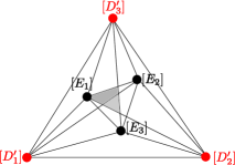
Figure 2. Divisorial valuations and flag complex $\Gamma$ arising from the resolution of the boundary $\bigcup_{i\in I}D_{i}$ at $p$ when $|I|=3$.

After picking a basis of the saturation in $\Lambda_{r}$ of the rank $s$ sublattice generated by $[\sigma_{I}]$, we may assume that $[D_{i}]=[D_{i}^{\prime}]=d_{i}e_{i}$ for all $i\in I$. Since the right-hand side of formula (4) is multiplicative with respect to each $d_{i}$, we may assume that $d_{i}=1$ for all $i\in I$. In this new coordinate system, we have $[E_{j}]=(m_{1j},\ldots,m_{sj})$ in $\mathbb{Z}^{s}$ for all $j=1,\ldots,u$, as in Figure 2.

Following Lemma 2.9, we wish to show that all regular points in the cone over the flag complex $\Gamma$ have weight $D_{1}\cdot\ldots\cdot D_{s}$. Consider a coarse fan structure $\mathcal{F}$ on the $s$-dimensional cone over the realization of $\Gamma$. For example, in Figure 2, this corresponds to having 12 vertices on the spherical complex induced by $\Gamma$: the six big dots, together with the six crossings of edges induced by the realization of $\Gamma$. Notice that the hyperplanes supporting facets in $\mathcal{F}$ are spanned by subsets of $\{[D_{i}^{\prime}]:i\in I\}\cup\{[E_{1}],\ldots,[E_{u}]\}$.

By construction, there are two types of cones to consider: the ones with a supporting hyperplane facet spanned by $s-1$ vertices in $\{D_{i}^{\prime}:i\in I\}$, and the ones that do not have this property. We prove our claim by a wall-crossing type formula in two steps. First, we show that the first type of cones have the expected weight. Second, we show that if a cone has the expected weight, the same is true for all its neighbors. Since the fan $\mathcal{F}$ is connected in codimension one by construction and the facets of $\sigma_{I}$ are generated by $s-1$ vertices in $\{v_{i}:i\in I\}$, this will prove our statement.

For simplicity, assume $I=\{1,\ldots,s\}$ and pick a cone spanned by $\{[D_{1}^{\prime}],\ldots,[D_{{s-1}}^{\prime}],[E_{j}]\}$ for some $j$. By formula (4), we know that the weight of this cone is the sum of the weight of all cells in $\Gamma$ whose cones contain the former. In particular,

(5) $$D_{1}^{\prime}\cdot\ldots\cdot D_{s}^{\prime}+\sum_{k=1}^{u}m_{sk}\,D_{1}^{\prime}\cdot\ldots\cdot D_{s-1}^{\prime}\cdot E_{k}=D_{1}^{\prime}\cdot\ldots\cdot D_{s-1}^{\prime}\cdot(D_{s}^{\prime}+\sum_{k=1}^{u}m_{sk}\,E_{k})=D_{1}^{\prime}\cdot\ldots\cdot D_{s-1}^{\prime}\cdot\pi^{*}(D_{s}),$$

since $m_{sk}$ is the index of the lattice spanned by $\{[D_{1}^{\prime}],\ldots,[D_{s-1}^{\prime}],[E_{j}]\}$ in its saturation. Since the resolution $\pi$ is a proper morphism, using the projection formula we have $\pi^{*}(D_{1})\cdot\ldots\cdot\pi^{*}(D_{s})=D_{1}\cdot\ldots\cdot D_{s}$ and $\pi^{*}(D_{i})\cdot W=0$ for all divisor $W$ contained in the exceptional locus. Thus, expression (5) equals $D_{1}\cdot\ldots\cdot D_{s}$ and so the first type of cones has the expected weight.

Now, pick two neighboring cones $\mathscr{C}_{1}$ and $\mathscr{C}_{2}$ with multiplicities $m_{\mathscr{C}_{1}}$ and $m_{\mathscr{C}_{2}}$ that intersect at a common facet $F$. For example, the shaded cells in Figure 2. Our goal is to show that $m_{\mathscr{C}_{1}}=m_{\mathscr{C}_{2}}$. For each $I_{0}\subset\{1,\ldots,s\}$ and $J_{0}\subset\{1,\ldots,u\}$ we call $D_{I_{0}}=\{D^{\prime}_{i}:i\in I_{0}\}$, $E_{J_{0}}=\{E_{j}:j\in J_{0}\}$ and $[D_{I_{0}}],[E_{J_{0}}]$ the associated semigroups in $\mathbb{Z}^{s}$. We consider all pairs $(I_{0},J_{0})$ such that the facet $F$ lies in the $(s-1)$-dimensional cone spanned by $[D_{I_{0}}]\cup[E_{J_{0}}]$, where $|I_{0}|+|J_{0}|=s-1$. By construction, every cone over a cell of $\Gamma$ containing $\mathscr{C}_{1}$ either also contains $\mathscr{C}_{2}$ or it intersects $\mathscr{C}_{2}$ only at the face $F$. Thus, we divide all maximal cones of $\mathbb{R}_{\geq 0}\Gamma$ into four types: the ones containing $\mathscr{C}_{1}\cup\mathscr{C}_{2}$, the ones containing $\mathscr{C}_{1}$ and not $\mathscr{C}_{2}$, the ones containing $\mathscr{C}_{2}$ but not $\mathscr{C}_{1}$, and the ones containing neither $\mathscr{C}_{1}$ nor $\mathscr{C}_{2}$ (see Figure 2). Cones of types two and three are spanned the $s-1$ rays in $[D_{I_{0}}]\cup[E_{J_{0}}]$, together with an extra ray. Formula (4) yields

(6) $$m_{\mathscr{C}_{1}}-m_{\mathscr{C}_{2}}=\sum_{I_{0},J_{0}}\big{(}\sum_{\begin{subarray}{c}\mathscr{C}\text{ of type 2}\\ \mathbb{R}_{\geq 0}\langle[D_{I_{0}}],[E_{J_{0}}]\rangle\prec\mathscr{C}\end{subarray}}m_{\mathscr{C}}\quad-\sum_{\begin{subarray}{c}\mathscr{C}\text{ of type 3}\\ \mathbb{R}_{\geq 0}\langle[D_{I_{0}}],[E_{J_{0}}]\rangle\prec\mathscr{C}\end{subarray}}m_{\mathscr{C}}\big{)},$$

where $\mathscr{C}$ is the cone over a maximal cell in $\Gamma$ and $\prec$ denotes the order in the face lattice of $\mathcal{F}$. Notice that the cone spanned by $[D_{I_{0}}]\cup[E_{J_{0}}]$ is a facet of $\mathscr{C}$. We prove that $m_{\mathscr{C}_{1}}-m_{\mathscr{C}_{2}}$ is zero by showing that for each pair $(I_{0},{J_{0}})$ the expression between parenthesis in (6) equals zero. Note that only cones of types two and three are involved.

First, we compute the weights of the cones $\mathscr{C}$. By definition, we have

$$m_{\mathscr{C}}=\begin{cases}D^{\prime}_{I_{0}}\cdot E_{J_{0}}\cdot D^{\prime}_{k}\,|\det([D_{I_{0}}]|[E_{J_{0}}]|[D^{\prime}_{k}])|&\text{ if }\mathscr{C}=\mathbb{R}_{\geq 0}\langle[D_{I_{0}}],[E_{J_{0}}],[D^{\prime}_{k}]\rangle,k\in I,\\ D^{\prime}_{I_{0}}\cdot E_{J_{0}}\cdot E_{l}\,|\det([D_{I_{0}}]|[E_{J_{0}}]|[E_{l}])|&\text{ if }\mathscr{C}=\mathbb{R}_{\geq 0}\langle[D_{I_{0}}],[E_{J_{0}}],[E_{l}]\rangle,l=1,\ldots u.\end{cases}$$

Here $D^{\prime}_{I_{0}}\cdot E_{J_{0}}\cdot D^{\prime}_{k}$ (resp. $D^{\prime}_{I_{0}}\cdot E_{J_{0}}\cdot E_{l}$) denotes the intersection number of the divisors in $D_{I_{0}}\cup E_{J_{0}}\cup\{D^{\prime}_{k}\}$ (resp. $D_{I_{0}}\cup E_{J_{0}}\cup\{E_{l}\}$).

Fix a pair $(I_{0},{J_{0}})$ such that the facet $F=\mathscr{C}_{1}\cap\mathscr{C}_{2}$ lies in the span of $[D_{I_{0}}]\cup[E_{J_{0}}]$. To simplify notation, assume $I_{0}$ consists of the last $|I_{0}|$ indices of $\{1,\ldots,s\}$. We fix the standard orientation of $\mathbb{R}^{s}$ and we label the set ${J_{0}}$ so that the ordered set $D_{I_{0}}\cup E_{J_{0}}$ satisfies that $\mathscr{C}_{1}$ lies in the positive half-space $F^{+}$ determined by the linear span of $F$, whereas $\mathscr{C}_{2}$ lies in the negative half-space $F^{-}$. This ensures that the determinant in the expression of the multiplicity $m_{\mathscr{C}}$ of a cone $\mathscr{C}$ of type two is positive, whereas for a cone of type three, this determinant is negative.

For any finite pair of ordered sets $A,B$, we let $\mathbb{S}(A,B)$ be set of injective functions from $A$ to $B$. Each element of $\mathbb{S}({A,B})$ has a sign induced by the corresponding element of the symmetric group on $|A|$ elements. Fix a cone $\mathscr{C}$ of type two spanned by $[D_{I_{0}}]\cup[E_{J_{0}}]\cup\{[D_{k}^{\prime}]\}$. Then, by expanding the determinant along the column associated to $[D_{k}^{\prime}]$, the multiplicity of $\mathscr{C}$ equals

$$m_{\mathscr{C}} =D_{I_{0}}\cdot E_{J_{0}}\cdot D^{\prime}_{k}\,(-1)^{s-|I_{0}|+1}\sum_{\alpha\in\mathbb{S}(J_{0},I\smallsetminus(I_{0}\cup\{k\}))}(-1)^{k+s-|I_{0}|}(-1)^{\operatorname{sign}(\alpha)}(\prod_{j\in{J_{0}}}m_{\alpha(j)j})$$

$$=(-1)^{1+k}\sum_{\alpha\in\mathbb{S}(J_{0},I\smallsetminus(I_{0}\cup\{k\}))}(-1)^{\operatorname{sign}(\alpha)}D_{I_{0}}\cdot\prod_{j\in{J_{0}}}(m_{\alpha(j)j}E_{j})\cdot D_{k}^{\prime}.$$

Likewise, by expanding determinants along the column $[E_{l}]$, a cone $\mathscr{C}$ of type two spanned by $[D_{I_{0}}]\cup[E_{J_{0}}]\cup\{[E_{l}]\}$ has multiplicity:

$$m_{\mathscr{C}}=\sum_{k\notin I_{0}}(-1)^{k+1}\sum_{\alpha\in\mathbb{S}(J_{0},I\smallsetminus I_{0})}(-1)^{\operatorname{sign}(\alpha)}D_{I_{0}}\cdot\prod_{j\in{J_{0}}}(m_{\alpha(j)j}E_{j})\cdot(m_{kl}E_{l}).$$

The formulas for the multiplicities of cones of type three will deferred from the previous ones in a sign, due to the orientation convention.

Notice that the previous formulas give the value zero when applied to cones that lie in the span of $[D_{I_{0}}]\cup[E_{J_{0}}]$. Therefore, if we fix $(I_{0},J_{0})$ and we add the contributions to (6) of the cones spanned by $[D_{I_{0}}]\cup[E_{J_{0}}]\cup\{[D_{k}^{\prime}]\}$ and the cones spanned by $[D_{I_{0}}]\cup[E_{J_{0}}]\cup\{[E_{l}]\}$ for all $k\notin I_{0}$ and $l=1,\ldots u$, we obtain

$$\sum_{k\in I\smallsetminus I_{0}}\;\sum_{\alpha\in\mathbb{S}(J_{0},I\smallsetminus(I_{0}\cup\{k\}))}(-1)^{1+k+\operatorname{sign}(\alpha)}\,D_{I_{0}}\cdot\underbrace{(D_{k}^{\prime}+\sum_{l=1}^{u}m_{kl}{E_{l}})}_{=\pi^{*}(D_{k})}\cdot\prod_{j\in{J_{0}}}(m_{\alpha(j)j}E_{j}).$$

By the projection formula, the previous expression equals 0. This concludes our proof. ∎

3. Tropical elimination and tropical implicitization

In this section we discuss tropical elimination and implicitization theory from the perspective of geometric tropicalization. Our exposition is based on [18, Section 5] and [19]. The overall spirit of tropical elimination lies in computing the tropicalization of the projection of a variety in $\mathbb{T}^{r}$ to a coordinate subspace $\mathbb{T}^{n}$. Tropical implicitization is a special instance of tropical elimination, where our (closed) input variety $X^{\prime}$ is the graph of a parameterization given by $n$ Laurent polynomials $\mathbf{f}=(f_{1},\ldots,f_{n})\colon X\subset\mathbb{T}^{d}\to\mathbb{T}^{n}$, i.e.

$$X^{\prime}:={\{(x,\mathbf{f}(x)):x\in X\}}\subset\mathbb{T}^{d+n},$$

and the monomial map $\alpha$ is the projection to the last $n$ coordinates of $\mathbb{T}^{d+n}$:

(7)

We aim to compute the tropical variety $\mathcal{T}\,\overline{\mathbf{f}(X)}$ from the geometry of $X$ and the polynomial map $\mathbf{f}$. For simplicity, we assume $\mathbf{f}$ is a generically finite map on $X$ of degree $\delta$. In what follows, we explain how to compute $\mathcal{T}\,\overline{\mathbf{f}(X)}$ from $\mathcal{T}X$ and the projection $\alpha$.

From now on, we fix $Y=\overline{\mathbf{f}(X)}\subset\mathbb{T}^{n}$. The variety $X^{\prime}\subset\mathbb{T}^{d+n}$ is a complete intersection. If we fix a basis of characters of $\mathbb{T}^{d+n}$, this variety is defined by the ideal $(y_{1}-f_{1}(x),\ldots,y_{n}-f_{n}(x))$ in $\mathbb{C}[x_{1}^{\pm 1},\ldots,x_{d}^{\pm 1},y_{1}^{\pm 1},\ldots,y_{n}^{\pm 1}]$. It is isomorphic to $X\subset\mathbb{T}^{n}$ via a monomial map and it projects to $Y$ through the dominant monomial map $\alpha$. Thus, tropical implicitization reduces to the task of computing $\mathcal{T}X^{\prime}$, which we do by means of geometric tropicalization.

Since $X\subset\mathbb{T}^{d}$ and $X^{\prime}\subset\mathbb{T}^{n+d}$ are isomorphic, we can choose to find a cnc pair for $X$ or $X^{\prime}$ and build the corresponding boundary complexes $\Delta(\partial\overline{X})$ or $\Delta(\partial\overline{X^{\prime}})$. The realization of the boundary complex in either $\Lambda_{d}$ or $\Lambda_{n+d}$ will reflect our choice. However, since $X$ is not a closed subvariety of $\mathbb{T}^{d}$ we would need to justify the correctness of this step. We do so in the proof of Theorem 3.1, whose set theoretic statement appeared already in [18, Corollary 2.9].

As in the previous section, we build a cnc pair $(\overline{X},\partial\overline{X})$ and its associated weighted boundary complex, of dimension $d-1$. The novelty with respect to the previous section will be our choice for a realization of this weighted complex in the cocharacter lattice $\Lambda_{n}$. A vertex $v_{i}$ of $\Delta(\partial\overline{X})$ gets assign the cocharacter $[\tilde{D_{i}}]:=\mathbf{f}^{\#}([D_{i}])=\operatorname{val}_{D_{i}}({\underline{\ \ }}\circ\mathbf{f})$, mapping a character $\chi$ to the lattice point $\operatorname{val}_{D_{i}}(\chi\circ\mathbf{f})$. If we fix a basis $\{\chi_{1},\ldots,\chi_{n}\}$ of characters in $\mathbb{T}^{n}$, the resulting cocharacter is represented by the lattice point $(\operatorname{val}_{D_{i}}(f_{1}),\ldots,\operatorname{val}_{D_{i}}(f_{n}))$. The realization of a maximal cell $\sigma_{I}\in\Delta(\partial\overline{X})$ in $\Lambda_{n}$ is the semigroup $[\tilde{\sigma_{I}}]$ spanned by $\{[\tilde{D_{i}}]:i\in I\}$. Note that the rank of $[\tilde{\sigma_{I}}]$ may drop. If this is not the case, we endow the semigroup $[\tilde{\sigma_{I}}]$ indexed by $I=\{i_{1},\ldots,i_{d}\}$ with the integer weight

(8) $$m_{[\tilde{\sigma_{I}}]}=\frac{1}{\delta}\,(D_{i_{1}}\cdot\ldots\cdot D_{i_{d}})\,\operatorname{index}(\mathbb{R}[\tilde{\sigma_{I}}]\cap\Lambda_{n},\mathbb{Z}[\tilde{\sigma_{I}}]),$$

where $\delta$ is the degree of the map $\mathbf{f}$. If the rank drops, we assign weight zero to the semigroup $[\tilde{\sigma_{I}}]$. The realization of $\Delta(\partial\overline{X})$ in $\Lambda_{n}$ is the collection of the weighted semigroups $\{[\tilde{\sigma_{I}}]:|I|=d\}$.

Theorem 3.1.

Let $\mathbf{f}\colon\mathbb{T}^{d}\dashrightarrow\mathbb{T}^{n}$ be a rational generically finite Laurent polynomial map and let $Y$ be the Zariski closure of the image of $\mathbf{f}$. Denote by $X\subset\mathbb{T}^{d}$ the domain of $\mathbf{f}$ and let $(\overline{X},\partial\overline{X})$ be a cnc pair with associated boundary complex $\Delta(\partial\overline{X})$. Then, the tropical variety $\mathcal{T}Y$ is the weighted cone over the realization of this complex in $\mathbb{R}\otimes\Lambda_{n}$.

Proof.

We now justify why we can compute $\mathcal{T}X^{\prime}\subset\mathbb{T}^{d+n}$ via finding a cnc pair for the open subset $X$ of $\mathbb{T}^{d}$. We build $\overline{X}$ in two steps. First, we add the boundary divisors $F_{1},\ldots,F_{n}$ of $\mathbb{T}^{d}$ given by the equations $f_{1},\ldots,f_{n}$. Then, we embed $\mathbb{T}^{d}$ inside a projective toric variety associated to the fan $\mathcal{T}X$ and we compactify $X$ inside this toric variety. By [21, Theorem 1.2], the outcome is a cnc pair $(\overline{X},\partial\overline{X})$. The components of the boundary $\partial\overline{X}$ come in two flavors: the divisors $\overline{F_{j}}$ obtained as the closure of $F_{j}$ in $\overline{X}$ and the divisors $D_{1},\ldots,D_{m}$ in $\overline{X}\smallsetminus\mathbb{T}^{d}$. Since $X^{\prime}$ is isomorphic to $X$, the cnc pair $(\overline{X},\partial\overline{X})$ is also associated to $X^{\prime}$. Notice that any choice of a cnc pair as this property. We choose a tropical compactification since the realization of the boundary complex is very explicit.

Next, we discuss out to realize the boundary complex $\Delta(\partial\overline{X})$ in $\Lambda_{d+n}$. For simplicity, we fix a basis $\{\chi_{1},\ldots\chi_{d},\zeta_{1},\ldots,\zeta_{n}\}$ of characters of the torus $\mathbb{T}^{d+n}$ by combining bases of characters of $\mathbb{T}^{d}$ and $\mathbb{T}^{n}$. Since $\chi_{i}$ is a unit in $\mathbb{T}^{d}$ and $\overline{F_{i}}\cap\mathbb{T}^{d}\subset\mathbb{T}^{d}$ is locally defined by $f_{i}(\mathbf{x})$, we have $\operatorname{val}_{\overline{F_{j}}}(\chi_{i})=0$, whereas $\operatorname{val}_{\overline{F_{j}}}(\zeta_{i})=\operatorname{val}_{\overline{F_{j}}}(f_{i})=\delta_{ij}$. Similarly, $\operatorname{val}_{D_{j}}(\zeta_{i})=\operatorname{val}_{D_{j}}(f_{i})$ for all $j$. Applying the projection $\alpha\colon\mathbb{R}^{d+n}\to\mathbb{R}^{n}$ to the last $n$ coordinates from (7), we see that each maximal cell $\sigma$ in $\Delta(\partial\overline{X})$ satisfies $\alpha([\sigma])=[\tilde{\sigma}]$. The transition from $\mathcal{T}X^{\prime}$ to $\mathcal{T}Y$ is obtained by applying the linear map $(0|\operatorname{Id}_{n})$ and noticing that

$$\operatorname{index}(\alpha([\sigma])^{\operatorname{sat}},\alpha([\sigma]))=\operatorname{index}(\alpha([\sigma])^{\operatorname{sat}},\alpha([\sigma]^{\operatorname{sat}}))\,\operatorname{index}([\sigma]^{\operatorname{sat}},[\sigma]),$$

unless the dimension of the vector space spanned by $\alpha([\sigma])$ is less than $d$. Such cones do not contribute to the multiplicity of regular points in $\mathcal{T}Y$.

We end by discussing the multiplicities on $\mathcal{T}Y$. By construction, $\delta$ equals the degree of the monomial map $\alpha$ restricted to the variety $X^{\prime}$. The push-forward formula of multiplicities implies the transition from (4) to (8) and in particular, the addition of the factor $1/\delta$ and the replacement of the lattice index factor in $\Lambda_{n+d}$ by the corresponding lattice index factor in $\Lambda_{n}$. ∎

It is in this sense that the boundary complex $\Delta(\partial\overline{X})$ is “pushed-forward” via the map $\mathbf{f}\colon X\to Y$ to give the boundary complex of a cnc pair associated to $Y$. The key fact in the proof of this result is that $\mathbf{f}$ induces a map on function fields $\mathbf{f}^{\#}\colon\mathbb{C}(Y)\hookrightarrow\mathbb{C}(X)$. Since the field $\mathbb{C}(X)$ is a finite extension of $\mathbb{C}(Y)$ of degree $\delta$, we can always extend any discrete valuation on $\mathbb{C}(Y)$ to a discrete valuation on $\mathbb{C}(X)$ via the map $\mathbf{f}^{\#}$. Likewise, valuations on $\mathbb{C}(X)$ can be restricted to $\mathbb{C}(Y)$. The realization of each vertex $v_{i}$ in $\Delta(\partial\overline{X})$ by the lattice point $[\tilde{D_{k}}]$ corresponds to the image of the realization of $D_{k}$ in $\Lambda_{n+d}$ under the linear map associated to the projection $\alpha$ from (7). This highlights the deep connections between tropical implicitization and homomorphisms of tori.

4. Tropical implicitization for generic surfaces

In this section, we specialize the constructions of Section 3 to the case of generic rational surfaces parameterized by polynomials with fixed support. Our methods are based on [19]. Unlike the case of [19, Theorem 4.1], our construction is independent on the smoothness on the ambient toric variety associated to a fan structure on the tropical variety. In addition, we give precise certificates for the genericity of these surfaces.

We keep the notation from Section 3. Our surface $Y\subset\mathbb{T}^{n}$ ($n\geq 3$) is parameterized by the generically finite Laurent polynomial map $\mathbf{f}=(f_{1},\ldots,f_{n})\colon\mathbb{T}^{2}\dashrightarrow\mathbb{T}^{n}$. Our goal is to compute the tropical surface $\mathcal{T}Y$. To simplify the exposition, we fix a basis of the character lattice $\Lambda_{n}^{\vee}$, which allows us to identify $\Lambda_{n}$ with $\mathbb{Z}^{n}$. Following [19], we assume each coordinate of $\mathbf{f}$ is generic relative to its support. That is, we fix the $n$ Newton polytopes $\mathcal{P}_{1},\ldots,\mathcal{P}_{n}$ of our polynomials $f_{1},\ldots,f_{n}$ and we let their coefficients vary generically. These $n$ polynomials determine $n$ curves in $\mathbb{T}^{2}$ with equations $(f_{i}=0)$. Our two main players in this section are the complement of this curve arrangement, which we call $X$, and the fan $\mathscr{N}$ obtained as the common refinement of the $n$ inner normal fans of the polytopes $\mathcal{P}_{1},\ldots,\mathcal{P}_{n}$. After compactifying $X$ inside the toric variety $X_{\mathscr{N}}$, the genericity condition guarantees that $(\overline{X},\partial\overline{X})$ is a cnc pair. The combinatorial nature of $X_{\mathscr{N}}$ makes it suitable for studying generic surfaces in the moduli space associated to the map $\mathbf{f}$.

We now state the main result in this section. The remainder will be devoted to its proof and to give several numerical examples. For simplicity, we assume that our choices of coefficients give distinct, irreducible polynomials. We denote the rays of $\mathscr{N}$ by $\rho_{1},\ldots,\rho_{m}$, oriented counterclockwise, with primitive generators $n_{\rho_{1}},\ldots,n_{\rho_{m}}$ in $\mathbb{Z}^{2}$. For each such ray $\rho\in\mathscr{N}^{[1]}$, we let $[D_{\rho}]=(\min_{\alpha\in\mathcal{P}_{1}}\{\alpha\cdot n_{\rho}\},\ldots,\min_{\alpha\in\mathcal{P}_{n}}\{\alpha\cdot n_{\rho}\})$. This is precisely the evaluation of the piecewise linear tropical map $\operatorname{trop}(\mathbf{f})$ at the point $\rho$.

Theorem 4.1.

The tropical variety $\mathcal{T}(Y)$ is the cone over a weighted graph, with vertices

$$\{e_{i}:\dim\mathcal{P}_{i}\neq 0,1\leq i\leq n\}\cup\{[D_{\rho}]:\rho\in\mathscr{N}^{[1]},[D_{\rho}]\neq 0\},$$

and positively weighted edges

1. $m_{([D_{\rho_{j}}],[D_{\rho_{k}}])}=\delta^{-1}{|\gcd\big{(}2\times 2-\operatorname{minors}\,([D_{\rho_{j}}]\mid[D_{\rho_{k}}])|}/{|\det(n_{\rho_{k}}\mid n_{\rho_{j}})|}$, if $|j-k|=1$ mod $m$ or $0$ otherwise.

2. $m_{(e_{i},[D_{\rho}])}=\delta^{-1}(|\operatorname{face}_{n_{\rho}}(\mathcal{P}_{i})\cap\mathbb{Z}^{2}|-1)\,\gcd\big{(}[D_{\rho}]_{j}:j\neq i\big{)}$, if $n_{\rho}\in\mathcal{T}(f_{i})$, or $0$ otherwise.

3. $m_{(e_{i},e_{j})}=\delta^{-1}\operatorname{length}((f_{i}=f_{j}=0)\cap\mathbb{T}^{2})$ if $\dim(\mathcal{P}_{i}+\mathcal{P}_{j})=2$, and $0$ otherwise. Under further genericity, this number equals $1/\delta$ times the mixed volume of $\mathcal{P}_{i}$ and $\mathcal{P}_{j}$.

It is important to point out that the previous algorithm was already presented in [19] and further studied in [18]. We contribute to the subject by elucidating the right genericity condition to impose. The proof of [19, Theorem 2.1] requires the genericity of both the coefficients and the Newton polytopes, to ensure that the Minkowski sum of the $n$ polytopes $\mathcal{P}_{1},\ldots,\mathcal{P}_{n}$ is a smooth polytope. Our proof discards this extra assumption on the polytopes, unraveling the key aspects in their argumentation, and extends the result to polynomial maps with arbitrary finite degree, as in [18, Theorem 5.1].

Proof.

We follow the strategy of [19, Theorems 2.1 and 4.1] and make the appropriate adjustments along the way. Our main tool will be Theorem 3.1. We fix the arrangement complement $X=\mathbb{T}^{2}\smallsetminus\bigcup_{i=1}^{n}(f_{i}=0)$ and embed it in the normal toric surface $X_{\mathscr{N}}$. The compactification of $X$ induces the pair $(X_{\mathscr{N}},\partial X_{\mathscr{N}})$, where

$$\partial X_{\mathscr{N}}=\{\overline{F_{1}},\ldots,\overline{F_{n}}\}\;\bigcup\;\{D_{1},\ldots,D_{m}\}.$$

Here, $D_{i}$ denotes the toric divisor $D_{\rho_{i}}$ and $\overline{F_{i}}$ is the divisor associated to the curve $F_{j}:=(f_{j}=0)$ in $\mathbb{T}^{2}$ as in the proof of Theorem 3.1.

The boundary $\partial X_{\mathscr{N}}$ consists of two types of irreducible components. The first class compounds the toric divisors indexed by the rays of $\mathscr{N}$. They correspond to facets of the Minkowski sum $\sum_{i=1}^{n}\mathcal{P}_{i}$. Since the fan $\mathscr{N}$ is simplicial, the toric boundary is a combinatorial normal crossings divisor. The remaining components are the $n$ divisors $\overline{F_{1}},\ldots,\overline{F_{n}}$, obtained from the curves $(f_{i}=0)$. The irreducibility and genericity of the polynomials $f_{i}$, together with Bertini’s theorem, show that these divisors are smooth and that $(X_{\mathscr{N}},\partial X_{\mathscr{N}})$ is a cnc pair. Notice that if $f_{j}$ consists of a single monomial, then $\overline{F_{j}}$ is the empty set. Such indices do not induce a vertex in the boundary complex $\Delta(\partial{X_{\mathscr{N}}})$, so from now on we may assume $\dim\mathcal{P}_{i}>0$ for all $i=1,\ldots,n$.

We now analyze the combinatorial information coming from the cnc pair. The boundary complex $\Delta(\partial X_{\mathscr{N}})$ is a graph with $m+n$ vertices. Its edges consist of pairs of vertices in $I\cup J$, where $I\subset\{1,\ldots,m\}$, $J\subset\{1,\ldots,n\}$. The first type of edges are of the form $(D_{\rho},D_{\rho^{\prime}})$ for $\rho$ and $\rho^{\prime}$ rays in the fan $\mathscr{N}$. By standard intersection theory on toric varieties, we know that the intersection numbers among the torus-invariant divisors are given by the following formula

(9) $$D_{\rho}\cdot D_{\rho^{\prime}}=\begin{cases}1&\;\operatorname{if}\,\rho\,\operatorname{and}\,\rho^{\prime}\,\operatorname{\text{generate a two-dimensional cone in }}\mathscr{N},\\ 0&\;\operatorname{else}.\end{cases}$$

This says that we only have edges among consecutive rays of $\mathscr{N}$, and their weight is 1.

When $|J|=1$, we seek to identify edges of the form $(\overline{F_{j}},D_{\rho})$, for $\rho\in\mathscr{N}$ and $j=1,\ldots,n$. Again, this is done by toric methods. Since $\overline{F_{j}}$ represents a Cartier divisor with local equation $f_{j}$, the weight of this edge is the intersection number of the initial form $\operatorname{in}_{{\rho}}(f_{j})$ and $D_{\rho}$. This quantity agrees with the number of nonzero solutions of the univariate polynomial $\operatorname{in}_{{\rho}}(f_{j})$, namely, the lattice length of the face of $\mathcal{P}_{j}$ associated to the ray $\rho$. If this face is a vertex, the initial form is a monomial, and so the intersection number is zero. Thus, we see that $\overline{F_{j}}$ is adjacent to a node $D_{\rho}$ if and only if ${\rho}$ is a ray in the normal fan of $\mathcal{P}_{j}$, and if so,

(10) $$\overline{F_{j}}\cdot D_{\rho}=\operatorname{\text{ lattice length of }}\operatorname{face}_{{\rho}}(\mathcal{P}_{j})=|\operatorname{face}_{{\rho}}(\mathcal{P}_{j})\cap\mathbb{Z}^{2}|-1.$$

Finally, if $|J|=2$, we want to certify which edges $(\overline{F_{i}},\overline{F_{j}})$ belong to the boundary complex $\Delta(\partial X_{\mathscr{N}})$. We claim it suffices to check if the equations $f_{i}$ and $f_{j}$ have a common root in $\mathbb{T}^{2}$ since any remaining intersection points would lie in the toric boundary, thus contradicting the cnc property of the chosen pair. Therefore, the weight of this edge is the length of the zero-dimensional scheme $(f_{i}=f_{j}=0)\cap\mathbb{T}^{2}$. If the coefficients of these polynomials are generic enough, Bernstein’s theorem implies that this number is the mixed volume of the polytopes $\mathcal{P}_{i}$ and $\mathcal{P}_{j}$. The mixed volume is nonzero if and only if the Minkowski sum of the corresponding polytopes is two-dimensional. This explains the extra assumption $\dim(\mathcal{P}_{i}+\mathcal{P}_{j})=2$ in the statement. Notice that since we are interested in the weighted boundary complex, we can safely assume that the dimension restriction characterizes the edges $(\overline{F_{i}},\overline{F_{j}})$. Artificial edges added to the boundary complex have weight zero.

It remains to discuss the realization of the boundary complex in $\mathbb{R}^{n}$. By Theorem 3.1, we know that $\operatorname{val}_{\overline{F_{j}}}(f_{i})=\delta_{i,j}$. We compute the divisorial valuation of all $D_{\rho}$’s with the tools of toric geometry [12, Section 5.2]. Without loss of generality, we may assume $n_{\rho}=e_{1}$. By definition, $\operatorname{val}_{D_{\rho}}(f_{j})$ is the order of vanishing of the polynomial $f_{j}$ at $D_{\rho}$, that is, by the maximal exponent of $x_{1}$ dividing $f_{j}$ in the polynomial ring $\mathbb{C}[x_{2}^{\pm 1}][x_{1}]$. Notice that this number can be negative. The maximum exponent is precisely $\operatorname{trop}(f_{j})(e_{1}):=\min_{\alpha\in\mathcal{P}_{j}}\{e_{1}\cdot\alpha\}$. We infer,

$$[D_{i}]:=(\operatorname{val}_{D_{i}}(f_{j}))_{j=1}^{n}=(\operatorname{trop}(f_{1})(n_{\rho_{i}}),\ldots,\operatorname{trop}(f_{n})(n_{\rho_{i}}))=\operatorname{trop}(\mathbf{f})(n_{\rho_{i}})\quad\forall\,i=1,\ldots,m.$$

Theorem 3.1, expressions (9) and (10) yield the desired multiplicities. ∎

Example 4.2.

Our first example is a modification of [19, Example 3.4], where we remove a monomial factor from each polynomial. This change has no effect on the combinatorics of the graph, but distorts its realization and the corresponding implicit equation. Our general surface $Y\subset\mathbb{T}^{3}$ is parameterized by

$$f_{1}(s,t)=a_{1}+a_{2}\,s^{2}t+a_{3}\,st^{2},\qquad f_{2}(s,t)=b_{1}\,st+b_{2}\,s+b_{3}\,t,\qquad f_{3}(s,t)=c_{1}\,t+c_{2}\,s^{2}+c_{3}\,st^{2},$$

where $a_{1},a_{2},a_{3},b_{1},b_{2},b_{3},c_{1},c_{2},c_{3}\in\mathbb{C}$ are generic nonzero coefficients. The map has degree $\delta=1$. The non-smooth fan $\mathscr{N}$ has nine rays but they yield only eight vertices in the realization of $\Delta(\partial\overline{X})$: $[D_{1}]=[D_{4}]=(-2,-1,-2),[D_{2}]=(-5,-3,-4),[D_{3}]=(-3,-2,-3),[D_{5}]=(-1,-1,-1),[D_{6}]=(0,-1,-1),[D_{7}]=(0,1,1),[D_{8}]=(0,1,2),[D_{9}]=(0,-1,-2)$. Likewise, the realization of the edges $(D_{6},D_{7})$ and $(D_{8},D_{9})$ in $\Delta(\partial X_{\mathscr{N}})$ give one-dimensional cones in $\mathcal{T}Y$. We indicate this by drawing a dashed edge in the abstract graph. The weights of all 19 edges are computed using mixed volumes, and are indicated in the left of Figure 3.

The resulting weighted graph in $\mathbb{R}^{3}$ has four bivalent vertices (in gray) and it is depicted on the right of Figure 3. After removing these gray vertices, we obtain a graph with $f$-vector $(7,13)$. The complement of the graph has eight connected components. Notice that the vertices $e_{2},[D_{1}]=[D_{4}],[D_{3}]$ and $[D_{5}]$ are aligned in the picture since they generate a two-dimensional cone in $\mathbb{R}^{3}$. In addition to the four bivalent vertices, this also explains the difference between the number of edges in the boundary complex and its realization. The predicted edge $([D_{4}],[D_{5}])$ can be seen as the arc containing the vertices $[D_{3}],[D_{4}]$ and $[D_{5}]$.

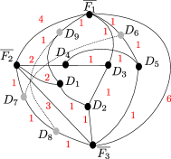
$\rightsquigarrow$

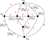
Figure 3. From left to right: weighted graphs representing $\mathcal{T}Y$. The left one corresponds to the abstract graph and the right one is the planar graph obtained by realizing the abstract graph and combining weights of overlapping edges. The dashed edges on the left graph have weight zero and they disappear in the planar graph.

For generic choices of coefficients $a_{1},\ldots,c_{3}$, the implicit polynomial has degree 14 [8]. Its Newton polytope has $f$-vector $(8,13,7)$, which matches the combinatorics of our graph. $\diamond$

Example 4.3.

We consider the morphism $f=(f_{1},f_{2},f_{3})\colon\mathbb{C}^{2}\dashrightarrow Y\subset\mathbb{C}^{3}$ given by

$$f_{1}(s,t)=a_{1}\,s^{2}+a_{2}\,s^{3}+a_{3}\,t^{2},\;f_{2}(s,t)=b_{1}\,t^{2}+b_{2}\,t^{3}+b_{3}\,s^{2},\;f_{3}(s,t)=c_{1}\,st+c_{2}\,s^{3}+c_{3}\,t^{3}+c_{4}\,st^{2}+c_{5}\,s^{2}t,$$

with generic coefficients $a_{1},\ldots,c_{5}\in\mathbb{C}^{*}$. The map has degree one and the normal fan $\mathscr{N}$ has eight rays, three of which have non-trivial weights 2, 2 and 3.

The vertices of the graph have coordinates $e_{1},e_{2},e_{3}$, $[D_{1}]=(0,0,0)$, $[D_{2}]=(-9,-6,-9)$, $[D_{3}]=(-3,-3,-3)$, $[D_{4}]=(-6,-9,-9)$, $[D_{5}]=(0,0,0)$, $[D_{6}]=(2,2,3)$, $[D_{6}]=(2,2,3)$, $[D_{7}]=(2,2,2)$ and $[D_{8}]=(2,2,3)$. After going through dimension testings, we obtain a list of fourteen edges as seen in the right of Figure 4, whose weights we can compute via mixed volumes. The transition from the weighted abstract graph to its realization is seen in Figure 4. $\diamond$

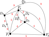
$\rightsquigarrow$

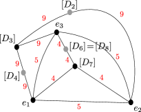
Figure 4. Weighted graphs representing $\mathcal{T}Y$.

Example 4.4.

As our third example we consider the surface in $\mathbb{C}^{3}$ parameterized by the degree one morphism $f=(f_{1},f_{2},f_{3})\colon\mathbb{C}^{2}\dashrightarrow Y$, where

(11) $$f_{1}(s,t)=a_{1}+a_{2}\,s+a_{3}\,t,\qquad f_{2}(s,t)=b_{1}+b_{2}\,t+b_{3}\,s^{2},\qquad f_{3}(s,t)=c_{1}+c_{2}\,st.$$

Using the methods described in this section we obtain a weighted graph with seven vertices $e_{1},e_{2},e_{3}$, $[D_{2}]=(-1,-2,0)$, $[D_{3}]=(-1,-2,-2)$, $[D_{4}]=(-2,-2,-3)$ and $[D_{5}]=(-1,-1,0)$. After removing the bivalent vertices $[D_{2}]$ and $[D_{5}]$, we get a graph with $f$-vector $(5,8)$, whose complement has five connected components. The eight edges are $(e_{1},e_{2})$, $(e_{1},e_{3})$ (both with weight 2), $(e_{2},e_{3})$ (with weight 3), $(e_{1},[D_{3}])$ (with weight 2), and $(e_{2},[D_{4}])$, $(e_{3},[D_{3}])$, $(e_{3},[D_{4}])$ and $([D_{3}],[D_{4}])$ (all with weight 1). Its support can be obtained from the rightmost picture in Figure 6 by removing the vertex $[E_{3}]$ and its three adjacent edges.

On the other hand, by standard elimination techniques, we see that the implicit equations is a dense polynomial of degree 3 in $x,y,z$ with five extreme monomials $1,x^{3},x^{2}y,y^{2}$ and $z^{2}$. Its coefficients are polynomials in the indeterminates $a_{1}$ through $c_{2}$. In Section 5 we revisit this example and explain how certain specializations of the coefficients $a_{1}$ through $c_{2}$ removes the extremal monomial $1$ and hence gives a new facet to the polytope. This choice of coefficients destroys the genericity conditions on the polynomial map $\mathbf{f}$. $\diamond$

5. Tropical implicitization for non-generic surfaces

In this section, we discuss methods for computing the tropicalization of non-generic parametric surfaces. As in Section 4, we start from a generically finite Laurent polynomial map $\mathbf{f}=(f_{1},\ldots,f_{n})\colon\mathbb{T}^{2}\dashrightarrow\mathbb{T}^{n}$. We assume that the polynomials have fixed support and we allow special choices of coefficients that preserve their Newton polytopes by such that $(X_{\mathscr{N}},\partial X_{\mathscr{N}})$ is not a cnc pair. We explain how to solve this issue and present numerical examples that illustrate the algebro-geometry complexity of the problem.

As we discussed in the generic case, we aim to find a cnc pair $(\overline{X},\partial\overline{X})$ associated to the arrangement of plane curves $X=\mathbb{T}^{2}\smallsetminus\bigcup_{i=1}^{n}(f_{i}=0)$. The following lemma implies that we can assume all $f_{i}$’s are irreducible. A similar result allows us to assume all polynomials are distinct.

Lemma 5.1.

Assume $\mathbf{f}$ is a finite map and that $f_{1}$ factors as $f_{1}=gh$ with $\deg g,\deg h<\deg f_{1}$. Then, the map $\mathbf{f^{\prime}}=(g,h,f_{2},\ldots,f_{n})\colon X\to\mathbb{T}^{n+1}$ is generically finite and $\mathbf{f}=\beta\circ\mathbf{f^{\prime}}$, where $\beta\colon\mathbb{T}^{n+1}\to\mathbb{T}^{n}$ sends $(t_{0},t_{1},\ldots,t_{n})$ to $(t_{0}t_{1},t_{2},\ldots,t_{n})$. In addition, $\beta$ restricted to the image of $\mathbf{f^{\prime}}$ is generically finite.

As a first attempt to answer our question, we apply generic methods from Section 4 and compactify $X$ via its embedding in the projective toric variety $X_{\mathscr{N}}$. The non-genericity of the coefficients of $\mathbf{f}$ says precisely that $(X_{\mathscr{N}},\partial X_{\mathscr{N}})$ is not a cnc pair. Since the excessive intersection points need not be torus invariant (and will not be in general), toric blow-ups cannot be used to achieve the desired condition. Instead, we can resolve toric singularities on the ambient space $X_{\mathscr{N}}$ by toric blow-ups, refining $\mathscr{N}$ to a smooth fan $\mathscr{N}^{\prime}$ in $\mathbb{R}^{2}$, perform classical point blow-ups on the smooth surface $X_{\mathscr{N}^{\prime}}$ and finally pull back the boundary divisors along this resolution. This procedure is tedious to do in practice. Our alternative strategy does not take advantage of the combinatorial input data, yet it is simpler to carry out in explicit calculations.

Given $\mathbf{f}$ and $X$ as above, we consider its compactification $\overline{X}$ in $\mathbb{P}^{2}$. This set has $n+1$ boundary divisors: $F_{i}=(f_{i}=0)$ and $F_{\infty}=(x_{3}=0)$. Let $\pi\colon\tilde{X}\to\overline{X}$ be any resolution of $\overline{X}$ obtained by blowing up all intersection points of three or more boundary components (if they exist), so that $(\tilde{X},\partial\tilde{X})$ is a cnc pair. Let $E_{1},\ldots,E_{s}$ be the corresponding exceptional divisors and $F_{\infty}^{\prime},F_{i}^{\prime}$ be the strict transforms of the divisors $F_{\infty},F_{i}$, $i=1,\ldots,n$. We write

$$\pi^{*}(F_{\infty})=F_{\infty}^{\prime}+\sum_{j=1}^{s}b_{j}E_{j},\qquad\pi^{*}(F_{i})=F_{i}^{\prime}+\sum_{j=1}^{s}b_{ij}\cdot E_{j},\quad i=1,\ldots,n,$$

for suitable $b_{ij},b_{j}\in\mathbb{Z}$. We let $\Gamma$ be the realized weighted boundary complex $\Delta(\partial\tilde{X})$ in $\mathbb{R}^{n}$. The vertices of $\Gamma$ are

$$[F_{\infty}^{\prime}]=(-\deg f_{1},\ldots,-\deg{f_{n}}),\qquad[F_{i}^{\prime}]=e_{i},\quad i=1,\ldots,n,$$

$$[E_{j}]=(b_{1j}-b_{j}\deg f_{1},\ldots,b_{nj}-b_{j}\deg f_{n}),\quad j=1,\ldots,s.$$

The weight of an edge $(v,w)$ equals

$$m_{(v,w)}=\frac{1}{\delta}\,i(v,w)\,\gcd(2\times 2-\operatorname{minors}(v\mid w)),$$

where $i(v,w)$ is the intersection number of the associated boundary divisors. An edge $(v,w)$ belongs to $\Gamma$ if it has positive weight. We conclude:

Theorem 5.2.

The tropical surface associated to the image of the map $\mathbf{f}\colon\mathbb{T}^{2}\dashrightarrow\mathbb{T}^{n}$ is the cone over the weighted graph $\Gamma$.

Before discussing the proof, it is instructive to analyze the transition from $\Delta(\partial\overline{X})$ to $\Delta(\partial\tilde{X})$. As we know, $\Delta(\partial\overline{X})$ contains a maximal cell $\sigma_{I}$ of dimension at least two. The index set $I$ corresponds to an intersection of $|I|$ boundary divisors. Any blow-up in this intersection produces a subdivision of $\delta_{I}$ (possibly removing boundaries), ultimately leading to a graph. At each step of the resolution, the excessive intersection point gives rise to an exceptional divisor and the remaining bad crossing points have lower multiplicity. The boundary complex $\Delta(\partial\tilde{X})$ is obtained by gluing all these resolution diagrams along common labeled vertices and also adding edges corresponding to pairwise intersections. The realization of this graph in $\mathbb{R}^{n}$ is read off from the proper transforms of the components of $\partial\overline{X}$.

Proof.

As explained earlier, our starting point is the naive compactification of $X$ in $\mathbb{P}^{2}$. We extend the map $\mathbf{f}$ by a homogeneous degree zero rational function $\mathbf{\tilde{f}}\colon\overline{X}\to Y$. Namely, $\tilde{f}_{i}=f_{i}^{h}/x_{0}^{\deg f_{i}}$ where $f_{i}^{h}$ is the homogenization of $f_{i}$ with respect to the new variables $x_{0}$.

The boundary $\partial\overline{X}$ has $n+1$ irreducible components: the $n$ divisors $F_{i}=(f_{i}^{h}=0)\subset\mathbb{P}^{2}$, $i=1,\ldots,n$ and the divisor at infinity $F_{\infty}=(x_{0}=0)$. By construction, the pull-back along $\mathbf{\tilde{f}}$ of the basis of characters $\{\chi_{1},\ldots,\chi_{n}\}$ is

$$\mathbf{\tilde{f}}^{*}(\chi_{j})=F_{j}+(-\deg f_{i})\cdot F_{\infty}\qquad j=1,\ldots,n.$$

Finally, we take a resolution $\pi\colon\tilde{X}\to\overline{X}$ by blowing up the excessive boundary intersection points. The set $\tilde{X}$ together with the map $g=\mathbf{\tilde{f}}\circ\pi$ gives us the desired cnc pair $(\tilde{X},\partial\tilde{X})$ and its realized boundary complex $\Delta(\partial\tilde{X})$. The result now follows from Theorem 3.1. ∎

The following two numerical examples illustrate Theorem 5.2. They correspond to special choices of coefficients in Examples 4.3 and 4.4. We show how the original boundary complexes and the induced tropical surfaces need to be modified in order to obtain the associated non-generic objects. To simplify notation, we let $s,t$ be our domain parameters and $u$ be the homogenizing variable.

Example 5.3.

We consider a particular choice of coefficients in Example 4.3. In this case, our degree one map is given by the following three bivariate polynomials:

$$f_{1}(s,t)=s^{2}-s^{3}-t^{2},\quad f_{2}(s,t)=t^{2}-t^{3}-s^{2},\quad f_{3}(s,t)=4st-s^{3}-t^{3}-3st^{2}-3s^{2}t.$$

Since our polynomials $f_{1},f_{2},f_{3}$ have nonnegative exponents, we consider $X=\mathbb{C}^{2}\smallsetminus\bigcup_{i=1}^{3}(f_{i}=0)$ and its compactification in $\mathbb{P}^{2}$. In this case, all three divisors intersect at the origin. After four blow-ups, we obtain the cnc pair $(\tilde{X},\partial\tilde{X})$.

Let $g=f\circ\pi\colon\tilde{X}\to Y$ be as in the proof of Theorem 5.2. Then, $g^{*}(\chi_{1})=F_{1}+2E_{1}+3E_{2}+3E_{3}+4E_{4}-3F_{\infty}$, $g^{*}(\chi_{2})=F_{2}+2E_{1}+3E_{2}+3E_{3}+4E_{4}-3F_{\infty}$, $g^{*}(\chi_{3})=F_{3}+2E_{1}+2E_{2}+2E_{3}+2E_{4}-3F_{\infty}$. Thus, $[F_{i}]=e_{i}$, $[F_{\infty}]=(-3,-3,-3)$, $[E_{1}]=(2,2,2)$, $[E_{2}]=[E_{3}]=(3,3,2)$, and $[E_{4}]=(4,4,2)$. The graph of $\mathcal{T}Y$ has six vertices and twelve edges and it is illustrated in Figure 5. Notice that the boundary complex $\Delta(\partial\tilde{X})$ has one bivalent vertex and two vertices $E_{2}$ and $E_{3}$ that map to the same integer vector. If we contract the divisor $E_{1}$ of $\tilde{X}$ that has negative self-intersection, we obtain a cnc pair with singularities whose boundary complex is build from $\Delta(\partial\tilde{X})$ by removing the bivalent vertex and merging the two edges $(F_{3},E_{1})$ and $(E_{1},E_{2})$ into a unique edge $(F_{3},E_{2})$. This shows that smoothness of the cnc pair is not required for geometric tropicalization.

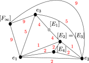
Figure 5. Weighted simplicial complex representing $\mathcal{T}Y$.

$\diamond$

Example 5.4.

We choose special parameter values for the map (11) in Example 4.4. The given non-generic surface $Y$ in $\mathbb{T}^{2}$ is parameterized by a degree one map:

(12) $$f_{1}(s,t)=-1-s+t,\qquad f_{2}(s,t)=-1+t-s^{2},\qquad f_{3}(s,t)=2-st.$$

This choice of coefficients eliminates the constant term from the implicit equation of $Y$ provided in Example 4.4 while preserving the supports of the three polynomials $f_{1},f_{2},f_{3}$. Hence, the graph has one extra vertex, associated to the extra facet that appears in the Newton polytope (see Figure 6). The compactification of $X=\mathbb{C}^{2}\smallsetminus\bigcup_{i=1}^{3}(f_{i}=0)$ in $\mathbb{P}^{2}$ has two triple intersection points: $(1:2:1)$ and $(0:1:0)$. Figure 6 shows the corresponding resolution diagrams. The realization of the boundary complex $\Delta(\partial\tilde{X})$ in $\mathbb{R}^{3}$ follows from the pullback of the basis of characters in $\mathbb{T}^{3}$:

$$\left\{\begin{aligned} (\mathbf{\tilde{f}}\circ\pi)^{*}(\chi_{1})&=F_{1}-F_{\infty}-E_{1}-2E_{2}+E_{3},\\ (\mathbf{\tilde{f}}\circ\pi)^{*}(\chi_{2})&=F_{2}-2F_{\infty}-E_{1}-2E_{2}+E_{3},\\ (\mathbf{\tilde{f}}\circ\pi)^{*}(\chi_{3})&=F_{3}-2F_{\infty}-E_{1}-3E_{2}+E_{3}.\end{aligned}\right.$$

Therefore, $[F_{i}]=e_{i}$ ($i=1,2,3$), $[F_{\infty}]=(-1,-2,-2)$, $[E_{1}]=(-1,-1,-1)$, $[E_{2}]=(-2,-2,-3)$ and $[E_{3}]=(1,1,1)$. In addition, the nonzero intersection multiplicities are $F_{1}\cdot F_{2}=F_{1}\cdot F_{3}=E_{1}\cdot F_{3}=E_{2}\cdot F_{2}=E_{2}\cdot F_{\infty}=E_{2}\cdot E_{3}=E_{3}\cdot F_{i}=1$ ($i=1,2,3$) and $F_{2}\cdot F_{3}=2$. By construction, we know that all edges have weight one, except for the edges $(e_{2},e_{3})$ and $(e_{1},[F_{\infty}])$, whose weight equals two. The resulting graph and the Newton polytope of the defining equation are shown in Figure 6.

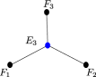
Figure 6. From left to right: Resolution diagrams at $(1:2:1)$ and $(0:1:0)$, Newton polytope and dual graph of the non-generic surface in $\mathbb{C}^{3}$ as in (12).

$\diamond$

As Theorem 5.2 show, the transition form the special to the generic case of tropical implicitization of surfaces can be done at the cost of resolving excessive intersections of plane curves. In addition to knowing the resolution diagrams, we need to carry the intersection numbers and divisorial valuations along the way. The examples presented show how hard it is to predict the combinatorics of the resolution by looking at the initial curve arrangement. The final divisorial valuations of the exceptional divisors heavily depend on the topology of the original plane curves.

The standard approach to obtain such valuations was introduced in work of Enriques and Chisini [10] and further developed with the notions of Enriques and dual diagrams [22]. Such methods are based on the topological type of the branches of the resolved curves. Furthermore, to compute pairwise intersection numbers of boundary divisors, we need to effectively compute this resolution, which is difficult to carry out in concrete examples. The main obstruction to predict these numbers without performing the resolution lies in the construction of clusters of infinitely near points of each singularity [5]. These clusters are precisely the point configurations emanating from successive blow-ups.

In the last years, a new object combining both Enriques and dual graphs was introduced by Popescu-Pampu under the name of kite [17]. In his language, clusters of infinitely near points are called constellations. This kite has a natural interpretation in the valuative tree of Favre and Jonsson [11] and it seems to provide the best framework to study arrangements of plane curves. We hope these tools will shed some light on tropical implicitization of non-generic surfaces.

References

- [1] L. Allermann and J. Rau. First steps in tropical intersection theory. Math. Z., 264(3):633–670, 2010.
- [2] M. Baker. Specialization of linear systems from curves to graphs. Algebra Number Theory, 2(6):613–653, 2008.
- [3] R. Bieri and J. R. J. Groves. The geometry of the set of characters induced by valuations. J. Reine Angew. Math., 347:168–195, 1984.
- [4] T. Bogart, A. N. Jensen, D. Speyer, B. Sturmfels, and R. R. Thomas. Computing tropical varieties. J. Symbolic Comput., 42(1-2):54–73, 2007.
- [5] A. Campillo, G. Gonzalez-Sprinberg, and M. Lejeune-Jalabert. Clusters of infinitely near points. Math. Ann., 306(1):169–194, 1996.
- [6] M. A. Cueto and S. Lin. Tropical secant graphs of monomial curves. In press, Beitr. Algebra Geom., 2012.
- [7] M. A. Cueto, E. A. Tobis, and J. Yu. An implicitization challenge for binary factor analysis. J. Symbolic Comput., 45(12):1296–1315, 2010.
- [8] W. Decker, G.-M. Greuel, G. Pfister, and H. Schönemann. Singular 3-1-1 – A computer algebra system for polynomial computations, 2010.
- [9] A. Dickenstein, E. M. Feichtner, and B. Sturmfels. Tropical discriminants. J. Amer. Math. Soc., 20(4):1111–1133 (electronic), 2007.
- [10] F. Enriques and O. Chisini. Lezioni sulla teoria geometrica delle equazioni e delle funzioni algebriche. 2. Vol. III, IV, volume 5 of Collana di Matematica [Mathematics Collection]. Nicola Zanichelli Editore S.p.A., Bologna, 1985. Reprint of the 1924 and 1934 editions.
- [11] C. Favre and M. Jonsson. The valuative tree, volume 1853 of Lecture Notes in Mathematics. Springer-Verlag, Berlin, 2004.
- [12] W. Fulton. Introduction to toric varieties, volume 131 of Annals of Mathematics Studies. Princeton University Press, Princeton, NJ, 1993. The William H. Roever Lectures in Geometry.
- [13] W. Fulton. Intersection theory, volume 2 of Ergebnisse der Mathematik und ihrer Grenzgebiete. 3. Folge. A Series of Modern Surveys in Mathematics [Results in Mathematics and Related Areas. 3rd Series. A Series of Modern Surveys in Mathematics]. Springer-Verlag, Berlin, second edition, 1998.
- [14] P. Hacking, S. Keel, and J. Tevelev. Stable pair, tropical, and log canonical compactifications of moduli spaces of del Pezzo surfaces. Invent. Math., 178(1):173–227, 2009.
- [15] J. Kollár. Lectures on resolution of singularities, volume 166 of Annals of Mathematics Studies. Princeton University Press, Princeton, NJ, 2007.
- [16] S. Payne. Boundary complexes and weight filtrations. arXiv:1109.4286, 2011.
- [17] P. Popescu-Pampu. Le cerf-volant d’une constellation. Ens. Math., 57:303–347, 2011.
- [18] B. Sturmfels and J. Tevelev. Elimination theory for tropical varieties. Math. Res. Lett., 15(3):543–562, 2008.
- [19] B. Sturmfels, J. Tevelev, and J. Yu. The Newton polytope of the implicit equation. Mosc. Math. J., 7(2):327–346, 351, 2007.
- [20] B. Sturmfels and J. Yu. Tropical implicitization and mixed fiber polytopes. In M. E. Stillman, N. Takayama, and J. Verschelde, editors, Software for Algebraic Geometry, volume 148 of I.M.A. Volumes in Mathematics and its Applications, pages 111–132, New York, 2008. Springer.
- [21] J. Tevelev. Compactifications of subvarieties of tori. Amer. J. Math., 129(4):1087–1104, 2007.
- [22] C. T. C. Wall. Singular points of plane curves, volume 63 of London Mathematical Society Student Texts. Cambridge University Press, Cambridge, 2004.