Universality of the Small-Scale Dynamo Mechanism

Abstract

We quantify possible differences between turbulent dynamo action in the Sun and the dynamo action studied in idealized simulations. For this purpose we compare Fourier-space shell-to-shell energy transfer rates of three incrementally more complex dynamo simulations: an incompressible, periodic simulation driven by random flow, a simulation of Boussinesq convection, and a simulation of fully compressible convection that includes physics relevant to the near-surface layers of the Sun. For each of the simulations studied, we find that the dynamo mechanism is universal in the kinematic regime because energy is transferred from the turbulent flow to the magnetic field from wavenumbers in the inertial range of the energy spectrum. The addition of physical effects relevant to the solar near-surface layers, including stratification, compressibility, partial ionization, and radiative energy transport, does not appear to affect the nature of the dynamo mechanism. The role of inertial-range shear stresses in magnetic field amplification is independent from outer-scale circumstances, including forcing and stratification. Although the shell-to-shell energy transfer functions have similar properties to those seen in mean-flow driven dynamos in each simulation studied, the saturated states of these simulations are not universal because the flow at the driving wavenumbers is a significant source of energy for the magnetic field.

1 INTRODUCTION

A turbulent 3-D flow in an electrically conducting fluid is capable of generating a magnetic field by self-excited dynamo action if the magnetic Reynolds number is sufficiently large. In the absence of rotation or large-scale shear flow, the energy of the generated magnetic field resides predominantly at spatial scales significantly smaller than the driving (integral) scale of the turbulence (Schekochihin et al., 2004). Such dynamos are therefore usually referred to as small-scale dynamos (SSDs). Turbulent plasmas are found in nearly all astrophysical systems. Since the big spatial scales of these systems imply large Reynolds numbers, SSDs are expected to operate in most of them. This leads to a widespread magnetization of astrophysical plasmas, the consequences of which can be profound (e.g., Schekochihin & Cowley, 2006; Wang & Abel, 2009; Schleicher et al., 2010; King & Pringle, 2010; Ryu et al., 2008).

Owing to their small-scale nature, observational evidence for magnetic fields generated by SSDs is difficult to obtain. Methods have been suggested to obtain information about the turbulent magnetic field in the interstellar and intracluster media (e.g., Waelkens et al., 2009). Evidence for such a field with mixed polarity on subresolution scales in the solar photosphere is obtained using the Hanle effect (Trujillo Bueno et al., 2004; Kleint et al., 2010) and, possibly, by considering the statistical properties of the resolved fields measured through the Zeeman effect (Pietarila Graham et al., 2009a, b).

Apart from these observational attempts, most research into SSDs has followed theoretical (e.g., Kazantsev, 1968) or numerical simulation approaches. Simulations of SSD action were carried out for a variety of physical settings, such as forced homogeneous incompressible turbulence (Meneguzzi et al., 1981), Boussinesq convection (Cattaneo, 1999), anelastic convection (Brun et al., 2004), up to fully compressible convection including relevant physics in the solar near-surface layers, such as radiative transport and partial ionization (Vögler & Schüssler, 2007; Pietarila Graham et al., 2010). Given such a range of physical conditions, the question arises of whether the mechanism of SSD action is universal or is qualitatively different in the presence of additional physics, e.g., as present in the near-surface layers of the Sun. In this paper, we therefore analyze three incrementally more complex simulations of SSDs, namely, (1) a simulation of forced homogeneous incompressible MHD turbulence, (2) a simulation of Boussinesq (incompressible) convection, and (3) a simulation of compressible and stratified solar near-surface convection. To compare the simulations, we consider energy spectra and shell-to-shell energy transfer rates in the kinematic growth phase and in the saturated state of the dynamo. Shell-to-shell energy transfer analyses measure the exchanges of kinetic and magnetic energies between different wavenumbers. In the case of incompressible MHD, the method has been well studied for dynamos as well as for decaying MHD flows (Dar et al., 2001; Debliquy et al., 2005; Mininni et al., 2005; Carati et al., 2006; Cho, 2010).

Schekochihin et al. (2007) have raised the question whether there is an essential physical difference between incompressible mean-flow-driven dynamos (Alexakis et al., 2005; Mininni et al., 2005) and those driven by random flows with correlation times shorter than their own turnover times. They suggested that, by measuring the shell-to-shell transfer of a dynamo resulting from using the latter forcing, one should be able to settle this question in the following way: if inertial-range motions dominate the amplification of the magnetic field, the dynamo is purely a property of the inertial range and independent of any system-dependent outer-scale circumstances. We call this condition universal in the Kolmogorov sense.

Schekochihin et al. (2007) were concerned about the large role of driving-scale motions in the dynamos studied by Alexakis et al. (2005); Mininni et al. (2005) and postulated these features were peculiar to the mean-flow driven case. However, Carati et al. (2006) studied a non-mean-flow-driven dynamo for the saturated state and found a strong nonlocal contribution from the forcing-scale motions to all scales of the magnetic field (as seen for mean-flow driving).

The paper is organized as follows. In Sect. 2, we describe the three simulation runs and give a brief account of the shell-to-shell analysis. This method requires a special treatment in the case of the solar convection simulation, which is described in Appendix A. The results of our analysis are reported in Sect. 3. We discuss them in Sect. 4 and give our conclusions in Sect. 5.

2 METHODS

2.1 Homogeneous Turbulence (HoT)

We use a pseudo-spectral FFT code (Gómez et al., 2005a, b; Mininni et al., 2010) to solve the incompressible MHD equations in a periodic box with $L=2\pi$,

$$\frac{\partial\boldsymbol{v}}{\partial t}+\boldsymbol{\omega}\times\boldsymbol{v}=-\boldsymbol{\nabla}p+\boldsymbol{j}\times\boldsymbol{b}+\nu\nabla^{2}\boldsymbol{v}+\boldsymbol{f},$$

$$\frac{\partial\boldsymbol{a}}{\partial t}=\boldsymbol{v}\times\boldsymbol{b}+\eta\nabla^{2}\boldsymbol{a},$$

$$\boldsymbol{\nabla}\cdot\boldsymbol{v}=\boldsymbol{\nabla}\cdot\boldsymbol{a}=0.$$ (1)

Here $\boldsymbol{\omega}=\boldsymbol{\nabla}\times\boldsymbol{v}$ is the vorticity. The magnetic field is given in Alfvénic units, $\boldsymbol{b}=\boldsymbol{\nabla}\times\boldsymbol{a}=\boldsymbol{B}/\sqrt{\rho\mu}$, with the vector potential $\boldsymbol{a}$ calculated in the Coulomb gauge. The forcing $\boldsymbol{f}$ is an Ornstein–Uhlenbeck process: the amplitudes of the complex harmonic modes with $2\leq\left|{\boldsymbol{k}}\right|\leq 3$ are evolved in time according to

$$C_{k_{x},k_{y},k_{z},t+\delta t}=C_{k_{x},k_{y},k_{z},t}\left(1-\frac{\delta t}{\tau_{\text{corr}}}\right)+\sqrt{\frac{2A}{\tau_{\text{corr}}}}\cdot\xi$$ (2)

where $\tau_{\text{corr}}$ is the correlation time (taken as unity), $A$ is chosen such that $v_{\text{rms}}\approx 1.1$, and $\xi$ is normally distributed noise with variance $\delta t$. The noise is randomized every time step, $\delta t=8\cdot 10^{-4}$. The values of the diffusivities are $\nu=\eta=8.8\cdot 10^{-4}$ in accordance with the resolution of the simulation which has $512^{3}$ modes (without de-aliasing). The integral scale of the motion is $L_{0}=1.9$, giving an integral-scale turnover time of $\tau_{L}=L_{0}/v_{\text{rms}}\approx 1.7$, and (kinetic and magnetic) Reynolds numbers $\mathit{Re}=\mathit{Re}_{\mathrm{m}}=v_{\text{rms}}L_{0}/\nu\approx 2400$. A non-magnetic simulation is run until a turbulent statistical steady state is reached after $\mathord{\approx}8\tau_{L}$; then, a seed field of harmonic modes in the range $20\leq\left|\boldsymbol{k}\right|\leq 30$ is introduced. After the kinematic phase of the magnetic field growth, the run is continued (initially with lower resolution and Reynolds numbers in order to save computing time) until a statistically stationary, saturated state is reached.

2.2 Boussinesq Convection (BC)

In the Boussinesq approximation the fluid is treated as incompressible except for the inclusion of buoyancy effects related to gravity. The nondimensionalized equations are

$$\frac{\partial\boldsymbol{\omega}}{\partial t}-\boldsymbol{\nabla}\times(\boldsymbol{v}\times\boldsymbol{\omega}+\boldsymbol{j}\times\boldsymbol{b})=\nu\nabla^{2}\boldsymbol{\omega}-\boldsymbol{\nabla}\theta\times\hat{\boldsymbol{g}},$$

$$\frac{\partial\boldsymbol{b}}{\partial t}-\boldsymbol{\nabla}\times(\boldsymbol{v}\times\boldsymbol{b})=\eta\nabla^{2}\boldsymbol{b},$$

$$\frac{\partial\theta}{\partial t}+(\boldsymbol{v}\cdot\boldsymbol{\nabla})\theta=\kappa\nabla^{2}\theta-(\boldsymbol{v}\cdot\boldsymbol{\nabla})T_{0},$$

$$\boldsymbol{\nabla}\cdot\boldsymbol{v}=\boldsymbol{\nabla}\cdot\boldsymbol{b}=0,\quad\boldsymbol{\nabla}\times\boldsymbol{b}=\boldsymbol{j}.$$ (3)

The temperature $\theta$ represents fluctuations about an equilibrium state with a mean vertical temperature gradient $\boldsymbol{\nabla}T_{0}$. The magnetic field is represented in Alfvénic units with an Alfvén number of one.

The BC simulation is a pseudospectral calculation performed at a resolution of $512^{3}$ in a fully periodic box. The amplitude of all modes with $k_{z}=0$ is set to zero to prevent the exponential growth of these modes (elevator instability, see Calzavarini et al., 2006) in the vertically periodic box. This non-restrictive “pseudo-Rayleigh–Bénard” boundary condition inhibits the formation of boundary layers that appear with Rayleigh–Bénard boundary conditions in a vertically closed box.

The BC simulation was carried out for a Prandtl number $\mathit{Pr}=\nu/\kappa=1$ and magnetic Prandtl number $\mathit{Pr}_{\mathrm{m}}=\nu/\eta=2$. The magnetic Reynolds number, defined in terms of the integral scale $L_{0}$ and $v_{\text{rms}}$ is $Re_{m}=v_{\text{rms}}L_{0}/\eta\approx 4000.$ The Rayleigh number is determined using the characteristic length-scale of the vertical temperature gradient and calculated to be $\mathit{Ra}=1/\nu\kappa=5.0\cdot 10^{5}$. Defined in this way, the Rayleigh number is not simply comparable to the Rayleigh number of a system with defined boundaries, but nevertheless gives an indication of the balance between buoyancy and dissipative forces in the simulation.

The initial state of the BC simulation consists of fully-developed hydrodynamic convection. Random fluctuations of magnetic field, small compared to the kinetic energy of the system, are seeded into the lowest 16 spectral modes in order to observe the onset of the linear phase where magnetic-field energy grows due to turbulent dynamo action. After nonlinear saturation the system enters an energetically quasi-stationary state.

2.3 Compressible Solar Convection

We use results from a dynamo simulation of near-surface solar convection carried out with the MURaM code (Vögler et al., 2005). The simulation differs from the more idealized simulations of MHD turbulence described above by including physical processes that are relevant for solar convection: compressibility, stratification, radiative energy transport, and partial ionization. The equations treated with the MURaM code, written in conservation form, are

$$\frac{\partial\varrho}{\partial t}+\boldsymbol{\nabla}\cdot(\varrho\boldsymbol{v})=0$$

$$\begin{split}\frac{\partial\varrho\boldsymbol{v}}{\partial t}+\boldsymbol{\nabla}\cdot\left[\varrho\boldsymbol{v}\boldsymbol{v}+\left(p+\frac{\left|\boldsymbol{B}\right|^{2}}{2\mu}\right)\mathds{1}-\frac{\boldsymbol{B}\boldsymbol{B}}{\mu}\right]\\ =\varrho\boldsymbol{g}+\boldsymbol{\nabla}\cdot\underline{\underline{\tau}},\end{split}$$

$$\frac{\partial\boldsymbol{B}}{\partial t}+\boldsymbol{\nabla}\cdot\left(\boldsymbol{v}\boldsymbol{B}-\boldsymbol{B}\boldsymbol{v}\right)=-\boldsymbol{\nabla}\times(\eta\boldsymbol{\nabla}\times\boldsymbol{B}),$$

$$\begin{split}\frac{\partial e}{\partial t}+\boldsymbol{\nabla}\cdot\left[\boldsymbol{v}\left(e+p+\frac{|\boldsymbol{B}|^{2}}{2\mu}\right)-\frac{1}{\mu}\boldsymbol{B}(\boldsymbol{v}\cdot\boldsymbol{B})\right]\\ =\frac{1}{\mu}\boldsymbol{\nabla}\cdot(\boldsymbol{B}\times\eta\boldsymbol{\nabla}\times\boldsymbol{B})+\boldsymbol{\nabla}\cdot(\boldsymbol{v}\cdot\underline{\underline{\tau}})\\ +\boldsymbol{\nabla}\cdot(K\boldsymbol{\nabla}T)+\varrho(\boldsymbol{g}\cdot\boldsymbol{v})+Q_{\text{rad}}.\end{split}$$ (4)

where $\varrho$ is the density, $p$ is the gas pressure, and $\boldsymbol{g}$ is the gravitational acceleration. $\boldsymbol{v}\boldsymbol{v}$, $\boldsymbol{B}\boldsymbol{B}$, $\boldsymbol{v}\boldsymbol{B}$ and $\boldsymbol{B}\boldsymbol{v}$ are dyadic products, and $\mathds{1}$ is the $3\times 3$ unit matrix. The viscous stress tensor, $\underline{\underline{\tau}}$, is written for a compressible medium with a viscosity coefficient containing a shock-resolving and a hyperdiffusive part (for details, see Vögler et al., 2005). The total energy density per volume, $e$, is the sum of internal, kinetic and magnetic energy densities. $T$ is the temperature and $K$ the thermal conductivity. The source term $Q_{\text{rad}}$, which accounts for radiative heating or cooling, is determined by integrating the equation of radiative transfer over a number of directions for each grid cell as described in Vögler et al. (2005). The system of equations is completed by the equation of state, which describes the relations between the thermodynamical quantities of a partially ionized fluid.

The numerical procedure uses centered, fourth-order explicit finite differences for the spatial derivatives on a uniform Cartesian grid and a fourth-order Runge–Kutta scheme for the time stepping. The boundary conditions are periodic in the horizontal directions with a closed, free-slip top boundary and an open lower boundary that permits the free in- and outflow of fluid (for details, see Vögler, 2003; Vögler et al., 2005).

Here we consider the results of the simulation that has previously been presented as Run C in Vögler & Schüssler (2007) and Run 2 in Pietarila Graham et al. (2010). The computational box represents a rectangular domain with an extent of $4.86\,\mathrm{Mm}$ in the horizontal directions and $1.4\,\mathrm{Mm}$ in the vertical direction, covering the range from $800\,\mathrm{km}$ below to $600\,\mathrm{km}$ above the optical solar surface. The finite-difference scheme uses $648\times 648\times 140$ grid cells, corresponding to a grid spacing of $7.5\times 7.5\times 10$ kilometers.

The magnetic Reynolds number for this simulation is $\mathit{Re}_{\mathrm{m}}=v_{\text{rms}}L_{0}/\eta\approx 2000$. Because the viscous stress tensor $\underline{\underline{\tau}}$ is based on shock-resolving and hyperdiffusivity, it is not simple to give explicit values of the Reynolds or magnetic Prandtl numbers. An estimate of the magnetic Prandtl number of between 1 and 2 was derived in Pietarila Graham et al. (2010) by considering the Taylor scales of the flow and magnetic field. The Reynolds number $\mathit{Re}$ is then in the range of 1000 to 2000.

2.4 Shell-to-Shell Transfer Analysis

This method was first derived for incompressible Navier-Stokes by Batchelor (1953) and for incompressible MHD by Dar et al. (2001). We follow here the exposition by Alexakis et al. (2005) who previously applied the analysis to kinematic and saturated dynamo states of homogeneous turbulence driven by a mean flow. We extend their study to random forcing as well as to more physically realistic simulations by deriving the compressible MHD shell-to-shell transfer functions.

The analysis starts with a decomposition of the velocity field and the magnetic field according to $\boldsymbol{a}(\boldsymbol{x})=\sum_{K}\boldsymbol{a}_{K}(\boldsymbol{x})$, where $\boldsymbol{a}_{K}$ is the part of $\boldsymbol{a}$ whose three-dimensional wave vector $\boldsymbol{k}$ in Fourier space lies in the range $K<\left|\boldsymbol{k}\right|\leq K+1$. The interval $(K,K+1]$ is referred to as “shell $K$”. Logarithmic binning $(\gamma^{n}K_{0},\gamma^{n+1}K_{0}]$ for $\gamma>1$ and integer $n$ is required to determine scale-to-scale energy transfers (Eyink & Aluie, 2009). However, we are not seeking to answer questions of scale locality of dynamo mechanisms (see, instead, Carati et al. 2006). Instead, we seek to determine whether the mechanism seen in incompressible homogeneous dynamos is also at work in our simulations.

For this purpose we use linear binning as opposed to the coarser analysis resulting from logarithmic binning; logarithmic binning can be recovered by summing over linear bins. The spectral rates of change of the kinetic and magnetic energies can then be written as

$$\frac{\partial}{\partial t}E_{\mathrm{v}}(K) =\sum_{Q}\bigl{[}\mathcal{T}_{\mathrm{vv}}+\mathcal{T}_{\mathrm{BvT}}+\mathcal{T}_{\mathrm{Iv}}\bigr{]}+\mathcal{F},$$ (5)

$$\frac{\partial}{\partial t}E_{\mathrm{B}}(K) =\sum_{Q}\bigl{[}\mathcal{T}_{\mathrm{BB}}+\mathcal{T}_{\mathrm{vBT}}+\mathcal{T}_{\mathrm{IB}}\bigr{]},$$ (6)

where $\mathcal{T}=\mathcal{T}(Q,K)$ are transfer functions:

$$\mathcal{T}_{\mathrm{vv}}(Q,K) =-\int\boldsymbol{v}_{K}(\boldsymbol{v}\cdot\boldsymbol{\nabla})\boldsymbol{v}_{Q}\,\mathrm{d}^{3}x,$$ (7)

$$\mathcal{T}_{\mathrm{BB}}(Q,K) =-\int\boldsymbol{B}_{K}(\boldsymbol{v}\cdot\boldsymbol{\nabla})\boldsymbol{B}_{Q}\,\mathrm{d}^{3}x,$$ (8)

$$\mathcal{T}_{\mathrm{BvT}}(Q,K) =\phantom{+}\int\boldsymbol{v}_{K}(\boldsymbol{B}\cdot\boldsymbol{\nabla})\boldsymbol{B}_{Q}\,\mathrm{d}^{3}x,$$ (9)

$$\mathcal{T}_{\mathrm{vBT}}(Q,K) =\phantom{+}\int\boldsymbol{B}_{K}(\boldsymbol{B}\cdot\boldsymbol{\nabla})\boldsymbol{v}_{Q}\,\mathrm{d}^{3}x.$$ (10)

$\mathcal{T}_{\mathrm{Iv}}$ and $\mathcal{T}_{\mathrm{IB}}$ represent the effects of dissipative heating, where the index “I” stands for internal energy. $\mathcal{F}=\mathcal{F}(K)$ corresponds to the contribution of external forces (e.g., gravity). The first two indices of the $\mathcal{T}$’s denote the energy reservoirs involved in the transfer; $\mathcal{T}_{\mathrm{rs}}(Q,K)$ is the rate of energy transferred from field $r$ in shell $Q$ to field $s$ in shell $K$. If $\mathcal{T}_{\mathrm{rs}}$ is positive, energy is received by $s$ from $r$ (transfer $Q\rightarrow K$). If it is negative, energy is lost by $s$ to $r$ (transfer $Q\leftarrow K$). The third index in $\mathcal{T}_{\mathrm{BvT}}$ and $\mathcal{T}_{\mathrm{vBT}}$ denotes the mediating force, in this case magnetic tension. Since Eqs. (7)–(10) express energy transfers from field $r$ in shell $Q$ to field $s$ in shell $K$, they satisfy the antisymmetry/conservation relations

$$\mathcal{T}_{\mathrm{rs}}(Q,K)=-\mathcal{T}_{\mathrm{sr}}(K,Q).$$ (11)

We now introduce the shell-to-shell transfer functions for compressible MHD. In the compressible case, there is work done by magnetic pressure, indicated by the index “P”. The work done by (or against) magnetic pressure cannot be separated from energy transferred between different wavenumbers inside the magnetic energy reservoir. Thus, the above system of shell-to-shell transfer functions cannot be used in the compressible case. As is consistent for antisymmetric pairings, we write instead:

$$\frac{\partial}{\partial t}E_{\mathrm{K}}(K) =\sum_{Q}\bigl{[}\mathcal{T}_{\mathrm{vv}}+\mathcal{T}_{\mathrm{BvP}}+\mathcal{T}_{\mathrm{BvT}}+\mathcal{T}_{\mathrm{Iv}}\bigr{]}+\mathcal{F},$$ (12)

$$\frac{\partial}{\partial t}E_{\mathrm{B}}(K) =\sum_{Q}\bigl{[}\mathcal{T}_{\mathrm{vBP}}+\mathcal{T}_{\mathrm{vBT}}+\mathcal{T}_{\mathrm{IB}}\bigr{]}.$$ (13)

In addition to viscous dissipation, $\mathcal{T}_{\mathrm{Iv}}$ now includes the internal energy transferred to the kinetic energy reservoir by compression. Pietarila Graham et al. (2010) show that this new transfer, $\mathcal{T}_{\mathrm{vBP}}$, accounts for 5% of the magnetic energy generated in the MURaM dynamo.

The transfer of magnetic energy in shell $Q$ to kinetic energy in shell $K$ through the magnetic tension force is

$$\mathcal{T}_{\mathrm{BvT}}(Q,K)=\frac{1}{2\mu}\int\bigg{[}\boldsymbol{v}_{K}\cdot(\boldsymbol{B}\cdot\boldsymbol{\nabla})\boldsymbol{B}_{Q}\\ +(\rho\boldsymbol{v})_{K}\cdot\left(\frac{\boldsymbol{B}}{\rho}\cdot\boldsymbol{\nabla}\right)\boldsymbol{B}_{Q}\bigg{]}\,\mathrm{d}^{3}x,$$ (14)

where the integral is taken over the analysis domain. The transfer of kinetic energy in shell $Q$ to magnetic energy in shell $K$ through the magnetic tension force is

$$\mathcal{T}_{\mathrm{vBT}}(Q,K)=\frac{1}{2\mu}\int\boldsymbol{B}_{K}\cdot\bigg{[}(\boldsymbol{B}\cdot\boldsymbol{\nabla})\boldsymbol{v}_{Q}\\ +(\boldsymbol{B}\cdot\boldsymbol{\nabla})\frac{(\rho\boldsymbol{v})_{Q}}{\rho}\bigg{]}\,\mathrm{d}^{3}x.$$ (15)

The transfers associated with magnetic pressure are

$$\begin{split}\mathcal{T}_{\mathrm{BvP}}(Q,K)=-\frac{1}{2\mu}\int\boldsymbol{B}\cdot\bigg{[}(\boldsymbol{v}_{K}\cdot\boldsymbol{\nabla})\boldsymbol{B}_{Q}\\ +\left(\frac{(\rho\boldsymbol{v})_{K}}{\rho}\cdot\boldsymbol{\nabla}\right)\boldsymbol{B}_{Q}\bigg{]}\,\mathrm{d}^{3}x,\end{split}$$ (16)

$$\begin{split}\mathcal{T}_{\mathrm{vBP}}(Q,K)=-\frac{1}{2\mu}\int\boldsymbol{B}_{K}\cdot\bigg{[}(\boldsymbol{v}_{Q}\cdot\boldsymbol{\nabla})\boldsymbol{B}\\ +\left(\frac{(\rho\boldsymbol{v})_{Q}}{\rho}\cdot\boldsymbol{\nabla}\right)\boldsymbol{B}+\boldsymbol{B}(\boldsymbol{\nabla}\cdot\boldsymbol{v}_{Q})\\ +\boldsymbol{B}\left(\boldsymbol{\nabla}\cdot\frac{(\rho\boldsymbol{v})_{Q}}{\rho}\right)\bigg{]}\,\mathrm{d}^{3}x.\end{split}$$ (17)

The transfers due to different force groupings, here magnetic tension (index T) and pressure (index P), separately satisfy the conservative antisymmetry relation, Eq. (11). The application to non-periodic boundaries (MURaM) necessitates a windowing of the data, described in detail in the Appendix.

3 RESULTS

3.1 Field Morphology and Energy Spectra

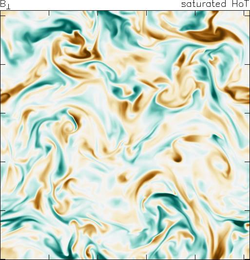
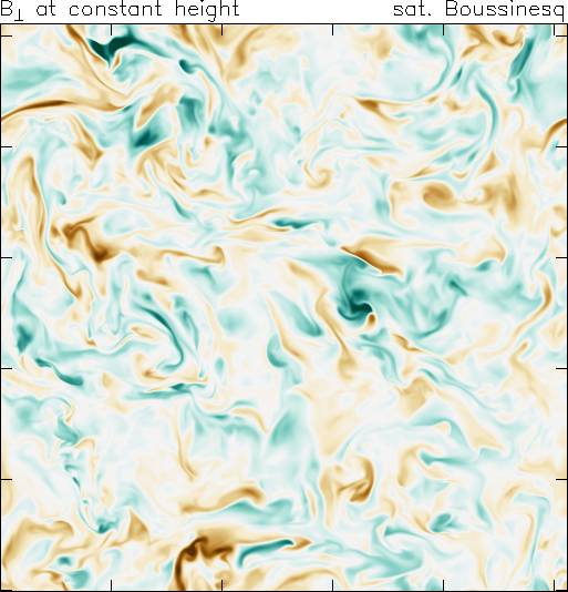
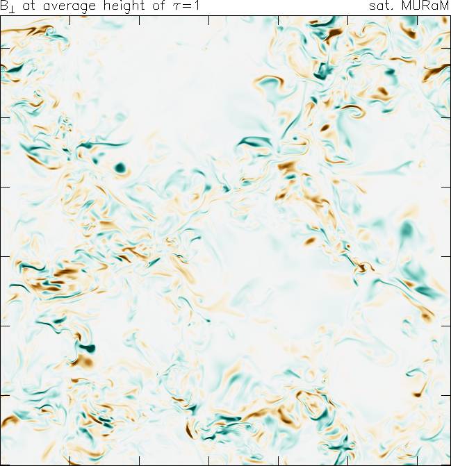
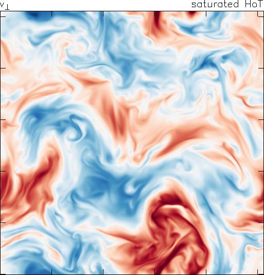
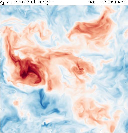
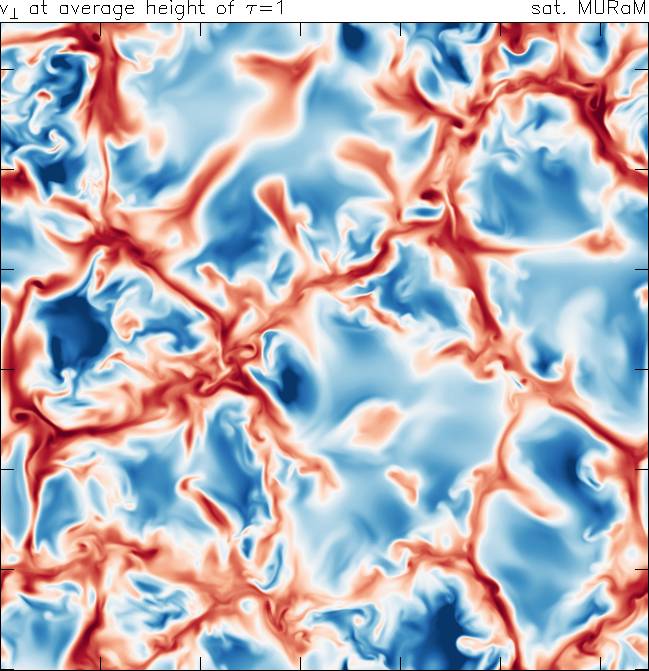
Figure 1: Maps of the vertical components of magnetic field (upper row) and fluid velocity (lower row) on horizontal cuts through each simulation box, taken from snapshots in the saturated dynamo state. The two magnetic polarities are shaded in turquoise and brown; white corresponds to zero vertical field. In the velocity maps, downflows are shaded red and upflows blue. Note that the arbitrary ratio of driving scale to box size is a factor of 3 smaller for MURaM.

In the saturated state, the ratio of total magnetic to total kinetic energy is 0.41 for HoT, 0.36 for BC, and 0.026 for MURaM. The small-scale dynamo is more efficient in the homogeneous cases HoT and BC. In the stratified solar case simulated with MURaM, the restriction of dynamo action to the downflow lanes and the losses due to downflows leaving the computational box limit the level of magnetic energy to a few percent of the kinetic energy. Figure 1 illustrates the structure of the velocity field and the dynamo-generated magnetic field in the saturated states of the three simulations. Shown are maps of the vertical magnetic field and velocity components on horizontal cuts. In all three cases, the magnetic field exhibits the typical folded structures arising from small-scale dynamo action, with elongated unipolar features and rapid polarity reversals in the transversal direction, often on a resistive spatial scale. While the field structures are fairly homogeneously distributed in the HoT and BC cases, the MURaM simulation shows an intermittent structure with extended patches almost devoid of field. This structure results from the up-down asymmetry of convection in a stratified medium: the convective upflows expand heavily in the horizontal directions and thus expel the magnetic flux. Thus in the MURaM simulation, magnetic field generation takes place mainly in the vicinity of the narrow turbulent downflows. The narrowness of these downflows and the size of the convection cells relative to the arbitrarily chosen size of the simulation box contribute to a smaller appearance of the magnetic field structures for MURaM presented in Figure 1.

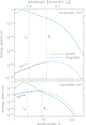
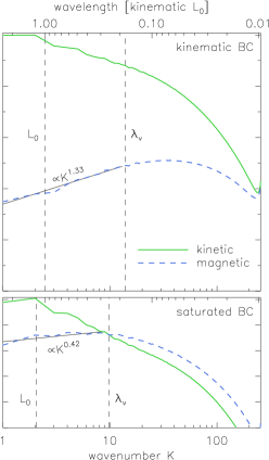
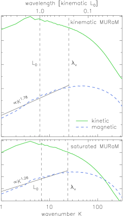
Figure 2: Kinetic and magnetic energy spectra in the kinematic (upper) and saturated (lower) states of the homogeneous turbulence (HoT) simulation (left), the Boussinesq convection (BC) simulation (center), and the solar convection (MURaM) simulation (right).

The greater separation between the driving scale and the box size can be quantified in the kinetic and magnetic energy spectra for the simulations shown in Fig. 2. Vertical lines indicate the integral scale for the turbulent motions,

$$L_{0}=\left.\int_{0}^{\infty}k^{-1}E_{\mathrm{v}}(k)\,\mathrm{d}k\middle/\int_{0}^{\infty}E_{\mathrm{v}}(k)\,\mathrm{d}k,\right.$$ (18)

and the Taylor microscale $\lambda_{\mathrm{v}}$,

$$\lambda_{\mathrm{v}}^{2}=\frac{\langle v^{2}\rangle}{\langle\omega^{2}\rangle}=\left.\int_{0}^{\infty}E_{\mathrm{v}}(k)\,\mathrm{d}k\middle/\int_{0}^{\infty}k^{2}E_{\mathrm{v}}(k)\,\mathrm{d}k.\right.$$ (19)

These scales signify the approximate beginning and end of the inertial range for a hydrodynamic or kinematic state. Both scales occur at higher wavenumbers for MURaM.

$(L_{0}/\lambda_{\mathrm{v}})^{2}$, which is proportional to the effective Reynolds number, is $31.5$ in the kinematic and $22.5$ in the saturated state of the Boussinesq simulation and $16.5$ ($10.1$) in the HoT simulation. The corresponding values for MURaM are $15.7$ and $12.7$, respectively. The spectra of all three dynamos are similar. In Fig. 2, the magnetic energy spectra exhibit power laws with positive exponents at small wavenumbers, peaking beyond $\lambda_{\mathrm{v}}$ in the kinematic state. The omni-directional spectra for MURaM are calculated employing a Tukey window (Harris, 1978) in the vertical direction. The window corresponds to a high-resolution/low-dynamic range apodization. This apodization increases spectral leakage from much stronger disparate frequencies such as the peak of kinetic energy at spatial frequency $L_{0}^{-1}$. Using a high-dynamic-range/low-resolution window such as the Nuttall window leads to similar spectral indices. In the stratified MURaM simulation, the anisotropic flow complicates any interpretation of the power law exponents. In the saturated state, magnetic energy dominates over kinetic energy for the largest wavenumbers and the peak of the spectrum moves to lower wavenumbers.

3.2 Shell-to-Shell Transfer

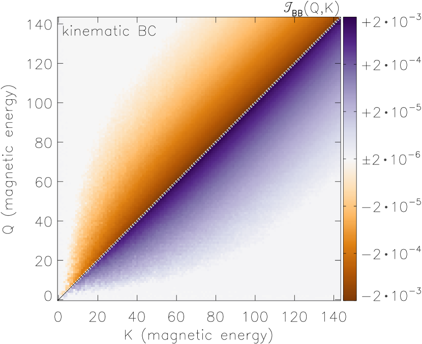
Figure 3: Shell-to-shell transfer from wavenumber $Q$ to wavenumber $K$ in the kinematic state of the BC simulation. Top: kinetic to kinetic energy. Bottom: magnetic to magnetic energy.

In order to compare the dynamo mechanism in our simulations, we need to look beyond visual and spectral similarities and measure in detail the generation of magnetic energy. To do this, we employ the shell-to-shell analysis described in Section 2.4.

As an example of how to interpret the transfer functions $\mathcal{T}(Q,K)$, Fig. 3 shows the cascade of kinetic and magnetic energy towards larger wavenumbers in the kinematic phase of the BC dynamo. In all of the plots, the transfer functions have been normalized by the maximum value of $\mathcal{T}_{\mathrm{vBT}}$ in the saturated state for each type of simulation. The normalization allows straightforward comparison of the relative changes in $\mathcal{T}_{\mathrm{vBT}}$, which is important for understanding the saturation mechanism of the dynamo. The normalization of all transfer functions for each type of simulation is consistent; however the absolute values of $\mathcal{T}_{\mathrm{vBT}}$ depend on the total amount of energy. Since the total energies vary between the simulations, the difference in the absolute magnitudes between simulations should not be compared. Instead we focus on qualitative comparisons and relative changes, both of which are not affected by the normalization. As the values of the different transfer functions vary strongly, the 2D plots have been constructed to extend over three orders of magnitude of positive and negative values. The absolute upper limit of the color map corresponds to the absolute maximum value of the represented $\mathcal{T}$.

In the top panel of Fig. 3, the transfer of kinetic energy from one shell to another, $\mathcal{T}_{\mathrm{vv}}(Q,K)$, is positive (indicated by purple color) for $Q\lesssim K$, i.e., shell $K$ receives energy from slightly smaller wavenumbers $Q$. $\mathcal{T}_{\mathrm{vv}}(Q,K)$ is negative (orange) for $Q\gtrsim K$, i.e., shell $K$ loses energy to slightly larger wavenumbers $Q$. Kinetic energy is transferred to larger wavenumbers as part of the local direct cascade of energy. This is seen also in the transfer of magnetic energy from one shell to another $\mathcal{T}_{\mathrm{BB}}(Q,K)$ (bottom panel). This picture is the same for both homogeneous (not shown) and Boussinesq convection and for both the kinematic and saturated (not shown) states (also compare with Fig. 3 of Mininni et al., 2005).

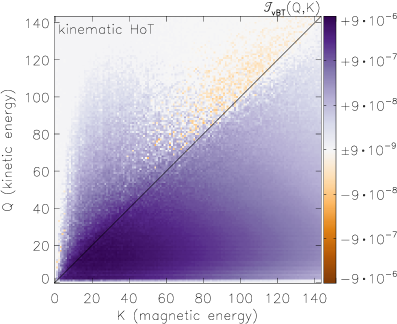
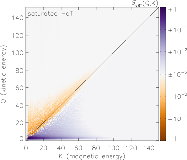
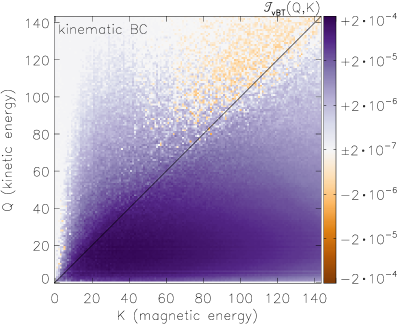
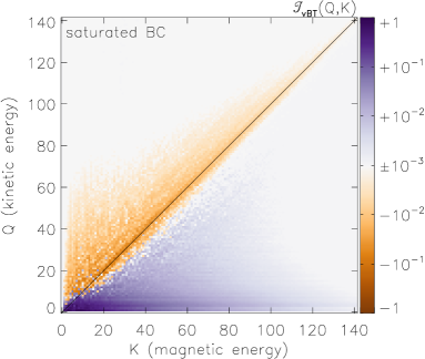
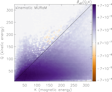
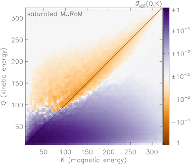
Figure 4: Shell-to-shell transfers for homogeneous turbulence (HoT, top panels), Boussinesq convection (BC, middle panels) and solar convection (MURaM, bottom panels). Shown are the transfers of kinetic energy at wavenumber shell $Q$ to magnetic energy at shell $K$, $\mathcal{T}_{\mathrm{vBT}}(Q,K)$, in the kinematic (left panels) and saturated states (right panels). Within each of the three types of simulations, a given set of arbitrary units is employed.

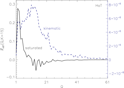
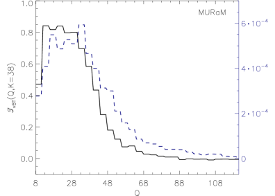
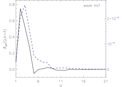
Figure 5: Cuts at constant $K\approx 1.3/\lambda_{\mathrm{v}}$ through the 2D maps in Figure 4 for the homogeneous turbulence (HoT) simulation (top left, $K=16$), the Boussinesq convection (BC) simulation (top right, $K=16$), the solar convection (MURaM) simulation (bottom left, $K=38$) and the weak homogeneous turbulence simulation ($E_{\text{mag}}=10\%E_{\text{kin}}$, $\mathit{Re}\approx 270$, bottom right, $K=5$). Solid lines correspond to the saturated state (left vertical axis) and dashed lines to the kinematic state (right vertical axis).

The kinematic dynamo mechanism is analyzed by measuring $\mathcal{T}_{\mathrm{vBT}}$, shown in panels on the left-hand side of Fig. 4. This transfer is positive for all $Q<K$, not just for nearby shells as in the cascade process in Fig. 3. All wavenumbers $Q<K$ of the fluid motion drive magnetic energy in a given shell $K$. This is the same as seen for dynamos driven by a mean flow (Mininni et al., 2005). Here, we see the same kinematic dynamo mechanism in all 3 simulations. At very large $Q>K$ corresponding to dissipative wavenumbers, there is less negative transfer in the MURaM case than in the other two cases, where it is already very weak. We conjecture that this difference is due to the differing treatment of viscosity in the codes.

The saturation of the dynamo results from the suppression of the velocity fluctuations at larger wavenumber by the back-reaction of the magnetic field on the flow through the Lorentz force. In the panels on the right-hand side of Figure 4 the transfer $Q\gtrsim K$ is negative (indicated by an orange color). This generalizes the result of Mininni et al. (2005) not only to random forcing in homogeneous turbulence, but also to incompressible convection and to realistic solar-like stratified convection. The wavenumber range where $\mathcal{T}_{\mathrm{vBT}}<0$ coincides with the range at which the magnetic energy spectrum dominates the kinetic energy spectrum (cf. Fig. 2). In MURaM, which has a lower saturated ratio $E_{\text{mag}}/E_{\text{kin}}\approx 2.6\%$ and a larger scale separation from the box size, this point occurs at significantly larger wavenumbers than for the other two simulations.

In the saturated state, there is a transfer of kinetic energy to higher wavenumber ($K>Q$) magnetic energy similar to that seen in the kinematic state. However, the transfer is more localized towards the small wavenumber $Q$ end of the kinetic energy spectrum (Alexakis et al., 2005; Mininni et al., 2005; Carati et al., 2006). For example, in the HoT simulation, the driving wavenumber for the fluid motions, $Q\approx 3$, is the dominant source for transfers to all $K$ in the saturated state.

Figure 5 presents vertical cuts at constant $K$ through the 2D maps of $\mathcal{T}_{\mathrm{vBT}}(Q,K)$ shown in Figure 4. These slices allow us to quantify the changes between the kinematic and the saturation regimes. For the MURaM dynamo, both the shift towards smaller $Q$ and the amount of negative transfer for $Q\gtrsim K$ is less dramatic than for the homogeneous and Boussinesq dynamos. This is reasonable because the MURaM dynamo is only slightly super-critical and thus the dynamo action is an order of magnitude weaker than in the other two simulations. If we were able to conduct the analysis for much larger $\mathit{Re}_{\mathrm{m}}$, the effect would become more pronounced. An additional HoT simulation performed in a regime similar to the MURaM dynamo confirms this interpretation. This additional weak HoT simulation was conducted at $\mathit{Re}=\mathit{Re}_{\mathrm{m}}\approx 270$ and $E_{\text{mag}}=10\%~{}E_{\text{kin}}$ in the saturated state. The MURaM dynamo transfers are shown next to similarly shaped transfers from the weak HoT in the lower panels of Fig. 5.

Figure 6: Cuts at constant $K$ through the 2D map in Figure 4 for the kinematic state of the homogeneous turbulence (HoT) simulation for $K=3$ (solid), $K=10$ (dashed), $K=20$ (dot-dashed), and $K=30$ (dotted).

In Fig. 5 a dominant peak at the driving wavenumber is absent in the kinematic state. Such a peak would be expected for a mean-flow driven incompressible dynamo (as seen in Fig. 6 of Mininni et al., 2005). For our randomly-forced HoT simulation (Fig. 6), we find that the total transfer to a given wavenumber $K$ increases with $K$, the transfer from kinetic energy at $Q\approx 3$ is no longer dominant for $K>3$, and the total transfer to $K\approx 3$ is dwarfed by the transfers to larger $K$. All three of these results present a view of randomly-forced dynamos that differs strongly from mean-flow driven dynamos. In particular, these results suggest that among small-scale turbulent dynamos randomly-forced dynamos are more local than mean-flow driven dynamos. Turbulent fluctuations play a greater role, for the kinematic phase, relative to integral-scale motions in the randomly-forced case than in either mean-flow-driven case of Mininni et al. (2005).

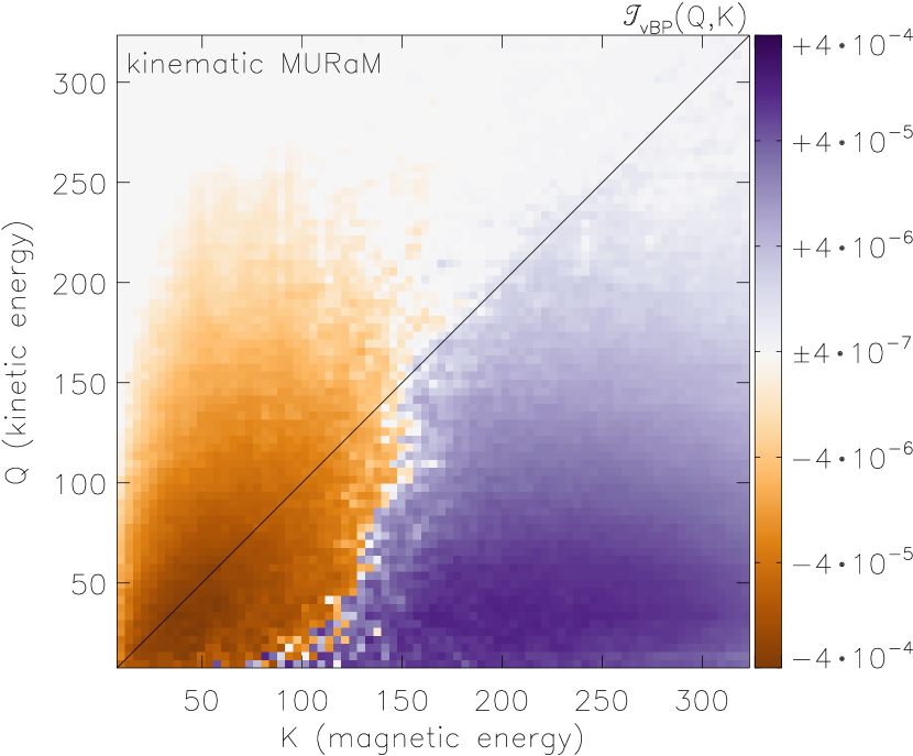
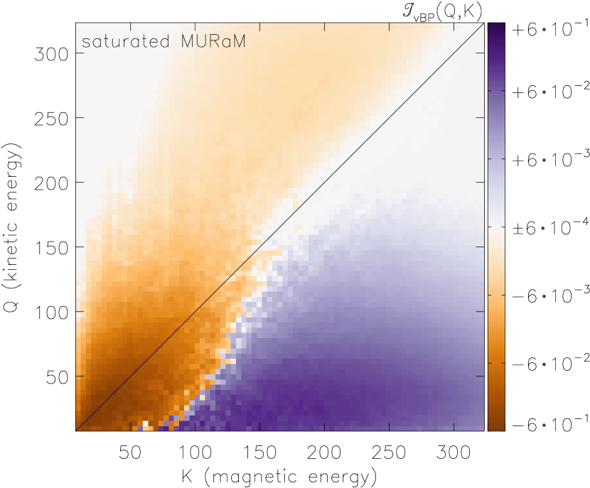
Figure 7: Shell-to-shell transfer of kinetic energy to magnetic energy in the solar (MURaM) simulation through the magnetic pressure gradient, $\mathcal{T}_{\mathrm{vBP}}$, in the kinematic phase (upper panel) and in the saturated state (lower panel).

Work against magnetic pressure becomes involved in the transport of magnetic energy from smaller to larger wavenumbers, a phenomenon often referred to as the magnetic energy cascade. For MURaM this cascade creates an imbalance resulting in an injection of 5% of the magnetic energy generated by the usual dynamo mechanism due to the magnetic tension force (Pietarila Graham et al., 2010). The shell-to-shell analysis of the transfer $\mathcal{T}_{\mathrm{vBP}}$ is shown in Fig. 7. Net energy is lost from small wavenumbers and deposited at larger wavenumbers. The transfer is not strongly dependent on the wavenumber $Q$ of the fluid motions up to a break-over point, $K\approx 100$. Magnetic energy at larger scales is expelled by the convection and compressed into the downflows. Quantitatively, $\mathcal{T}_{\mathrm{vBP}}$ is stronger for smaller $Q$, indicating the importance of motions at the convective scales for the flux expulsion process. At larger wavenumbers, magnetic energy is generated by fluid motions at smaller wavenumber, e.g., through work against the magnetic pressure, and lost to motions at larger wavenumbers, such as viscously damped magnetosonic waves.

4 DISCUSSION

In the three simulations presented here, turbulent flows are driven by different mechanisms: random forcing (HoT), Boussinesq convection (BC) and radiative cooling-driven convection (MURaM). The HoT and BC cases are very similar in all aspects. This includes the structure of the flow and magnetic field (Fig. 1), the energy spectra (Fig. 2) and the energy transfer spectra (Fig. 4). The similarity is not surprising considering that the only essential difference between the simulations is the phase information contained in the large-scale driving function.

The outer-scale appearance of the MURaM simulation is different from the other two cases (Fig. 1). There is a strong asymmetry between the upflowing and the downflowing plasma, with relatively smooth upflows and narrow, highly turbulent downflows. Also, the arbitrary ratio between the box size and the driving scale is a factor 3 larger. In spectral space, this corresponds to a shift towards higher wavenumbers. The shift affects the peaks of the kinetic energy (Fig. 2) and the kinematic transfer functions (Fig. 5). Since the $e$-folding time of the magnetic energy in the kinematic regime is significantly shorter than the turnover time of the granular convection, most of the magnetic field appears in the downflow lanes.

The shell-to-shell energy transfer functions (Fig. 4) are similar in the kinematic state, in particular transfer from the inertial range wavenumbers is dominant. This suggests that the dynamo mechanism, namely the turbulent shear stress of the motions in the inertial range, is essentially the same in each of the cases studied. Neither the short correlation time of random forcing nor the additional physics, as present in the Sun, alter the dynamo mechanism previously discovered in incompressible turbulence with a mean flow. As a property of the inertial range, independent of system-dependent outer-scale circumstances, the dynamo mechanism is universal in the Kolmogorov sense.

In the saturated state, the transfers involve much stronger energy transfer from flows at the driving wavenumber. This is particularly true for the strongly supercritical HoT and BC cases. Since the flow at these wavenumbers is determined by the large-scale driving, the dynamo action is no longer universal in the sense defined above.

The structure of magnetic fields produced by the small-scale dynamo for magnetic Prandtl number $\mathit{Pr}_{\mathrm{m}}\ll 1$ is different than for $\mathit{Pr}_{\mathrm{m}}>1$ (Schekochihin et al., 2007). We have shown that buoyancy and stratification do not significantly alter the small-scale dynamo mechanism. Since small-scale dynamo action is known to work for $\mathit{Pr}_{\mathrm{m}}\ll 1$ in incompressible MHD (Ponty et al., 2005; Schekochihin et al., 2007) and with the same shell-to-shell transfer mechanism down to at least $\mathit{Pr}_{\mathrm{m}}\approx 0.5$ (Alexakis et al., 2007), we expect small-scale dynamo action to be possible for $\mathit{Pr}_{\mathrm{m}}\ll 1$ both for MURaM and the Sun.

5 CONCLUSIONS

We have compared simulations of solar magneto-convection and local dynamo action with the properties of idealized systems in order to evaluate the robustness and the range of applicability of the conclusions drawn from studying the idealized models. The dynamo has similar shell-to-shell energy transfer properties for homogeneous-isotropic-incompressible turbulence, Boussinesq convection, and solar conditions that include stratification, compressibility, partial ionization and radiative energy transport. The results suggest that the dynamo mechanisms, namely, turbulent shear stresses acting in the inertial range, operate in the same way in each of the cases considered.

For incompressible turbulence we find many similarities in the dynamo generated by random forcing with a correlation time shorter than its turnover time and that resulting from mean-flow driving previously reported (Alexakis et al., 2005; Mininni et al., 2005). While the signature of the dynamo mechanism is the same, the role of forcing-wavenumber fluid motions is diminished when random forcing is used for the kinematic phase. For the saturated state, injection from forcing-wavenumbers remains significant even for random forcing (similar to what was found by Carati et al. 2006 for yet another type of forcing). Basic properties of the turbulent small-scale dynamo process have been thoroughly studied for homogeneous, isotropic, triply-periodic simulations; these properties carry over to two situations that include more complex physics: Boussinesq convection and solar surface convection.

Appendix A Shell-to-Shell Analysis for MURaM

The use of discrete Fourier transforms is complicated by the non-periodicity of the MURaM data in the vertical direction. Ringing effects may seriously taint the transfer functions. We prevent ringing effects in this calculation by applying a 50% Tukey window (Harris, 1978) on the data in the vertical direction before the transfer analysis. In addition, we zero-pad beyond the extent of the original data to exclude wrap-around effects.

We apply the usual shell filter decomposition $\boldsymbol{a}(\boldsymbol{x})=\sum_{K}\boldsymbol{a}_{K}(x)$ to velocity $\boldsymbol{v}$, momentum $\rho\boldsymbol{v}$ and the magnetic field $\boldsymbol{B}$, as described in Sect. 2.4 but with a shell width of 4. When computing the isotropic wavenumber $K$, we relate all components of $\boldsymbol{k}$ to horizontal wavelengths, i.e., $K=1$ corresponds to one wave cycle in one of the two axes-aligned horizontal directions. The antisymmetry relations, Eq. (11), are satisfied analytically, both for periodic boundary conditions and if a window is applied which tapers off to zero at the boundary. In general, a surface integral contribution must be applied.

To assess the reliability of the transfers computed in this way, we performed a series of tests using the results of a low-resolution HoT run. In its original form, the data is fully periodic and the transfer analysis is correct by definition. If we “truncate” the data by zeroing half of the box in one direction, the transfer analysis results in spurious power at high frequencies in the form of ringing noise, see Fig. 8. If, in addition, a window is applied to the data, the results obtained are similar to the original. As is illustrated in Fig. 9, the slopes and amplitudes are reasonably well approximated. The tests indicate that the transfer functions can be trusted within the scope of the study presented in this paper.

The disparity between the vertical and horizontal extent of the computational domain corrupts the transfer functions at low wavenumbers $K,Q\lesssim 7$. These large-scale modes either do not exist in the vertical direction or are directly affected by the alteration of the data by the window. $K\approx 7$ corresponds to the vertical extent of the unaltered part of the data. In the plots of the transfers for MURaM (Figs. 4, 5, and 7), only wavenumbers above 8 are shown.

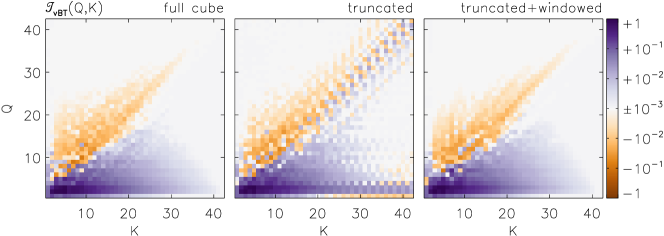
Figure 8: Transfer function in a $128^{3}$ HoT simulation computed in three different ways: using the original periodic cube (left), using a cube in which half of the data has been zeroed (middle) and using a “half-zeroed” cube with the remaining data being forced to be periodic by a Tukey window (right). The results have been renormalized to account for the impact of the truncation and windowing on the amplitude.

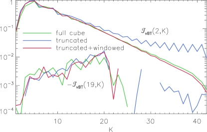
Figure 9: Cuts through the transfer functions shown in Fig. 8.

References

- Alexakis et al. (2005) Alexakis, A., Mininni, P. D., & Pouquet, A. 2005, Phys. Rev. E, 72, 046301
- Alexakis et al. (2007) Alexakis, a., Mininni, P. D., & Pouquet, a. 2007, New Journal of Physics, 9, 298
- Batchelor (1953) Batchelor, G. K. 1953, The Theory of Homogeneous Turbulence (Cambridge University Press)
- Brun et al. (2004) Brun, A. S., Miesch, M. S., & Toomre, J. 2004, ApJ, 614, 1073
- Calzavarini et al. (2006) Calzavarini, E., Doering, C. R., Gibbon, J. D., Lohse, D., Tanabe, A., & Toschi, F. 2006, Phys. Rev. E, 73, 035301
- Carati et al. (2006) Carati, D., Debliquy, O., Knaepen, B., Teaca, B., & Verma, M. 2006, Journal of Turbulence, 7, 51
- Cattaneo (1999) Cattaneo, F. 1999, ApJ, 515, L39
- Cho (2010) Cho, J. 2010, ApJ, 725, 1786
- Dar et al. (2001) Dar, G., Verma, M. K., & Eswaran, V. 2001, Physica D Nonlinear Phenomena, 157, 207
- Debliquy et al. (2005) Debliquy, O., Verma, M. K., & Carati, D. 2005, Physics of Plasmas, 12, 042309
- Eyink & Aluie (2009) Eyink, G. L. & Aluie, H. 2009, Physics of Fluids, 21, 115107
- Gómez et al. (2005a) Gómez, D. O., Mininni, P. D., & Dmitruk, P. 2005a, Advances in Space Research, 35, 899
- Gómez et al. (2005b) —. 2005b, Physica Scripta Volume T, 116, 123
- Harris (1978) Harris, F. J. 1978, IEEE Proceedings, 66, 51
- Kazantsev (1968) Kazantsev, A. P. 1968, Soviet Journal of Experimental and Theoretical Physics, 26, 1031
- King & Pringle (2010) King, A. R. & Pringle, J. E. 2010, MNRAS, 404, 1903
- Kleint et al. (2010) Kleint, L., Berdyugina, S. V., Shapiro, A. I., & Bianda, M. 2010, A&A, 524, A37
- Meneguzzi et al. (1981) Meneguzzi, M., Frisch, U., & Pouquet, A. 1981, Physical Review Letters, 47, 1060
- Mininni et al. (2005) Mininni, P., Alexakis, A., & Pouquet, A. 2005, Phys. Rev. E, 72, 046302
- Mininni et al. (2010) Mininni, P. D., Rosenberg, D. L., Reddy, R., & Pouquet, A. 2010, arXiv:1003.4322v1 [physics.comp-ph]
- Pietarila Graham et al. (2010) Pietarila Graham, J., Cameron, R., & Schüssler, M. 2010, ApJ, 714, 1606
- Pietarila Graham et al. (2009a) Pietarila Graham, J., Danilovic, S., & Schüssler, M. 2009a, in Astronomical Society of the Pacific Conference Series, Vol. 415, Astronomical Society of the Pacific Conference Series, ed. B. Lites, M. Cheung, T. Magara, J. Mariska, & K. Reeves, 43
- Pietarila Graham et al. (2009b) Pietarila Graham, J., Danilovic, S., & Schüssler, M. 2009b, ApJ, 693, 1728
- Ponty et al. (2005) Ponty, Y., Mininni, P., Montgomery, D., Pinton, J.-F., Politano, H., & Pouquet, a. 2005, Physical Review Letters, 94, 2
- Ryu et al. (2008) Ryu, D., Kang, H., Cho, J., & Das, S. 2008, Science, 320, 909
- Schekochihin & Cowley (2006) Schekochihin, A. A. & Cowley, S. C. 2006, Physics of Plasmas, 13, 056501
- Schekochihin et al. (2004) Schekochihin, A. A., Cowley, S. C., Taylor, S. F., Maron, J. L., & McWilliams, J. C. 2004, ApJ, 612, 276