Large scale environmental bias of the QSO line of sight proximity effect

Abstract

We analyse the overionisation or proximity zone of the intergalactic matter around high-redshift quasars in a cosmological environment. In a box of $64\;h^{-1}\textrm{ Mpc}$ base length we employ high-resolution dark matter only simulations with $1024^{3}$ particles. For estimating the hydrogen temperature and density distribution we use the effective equation of state by Hui & Gnedin (1997). Hydrogen is assumed to be in photoionisation equilibrium with a model background flux which is fit to recent observations of the redshift dependence of the mean optical depth and the transmission flux statistics. At redshifts $z=3,4,\mbox{and }4.8$, we select model quasar positions at the centre of the 20 most massive halos and 100 less massive halos identified in the simulation box. From each assumed quasar position we cast 100 random lines of sight for two box length including the changes in the ionisation fractions by the QSO flux field and derive mock Ly$\alpha$ spectra. The proximity effect describes the dependence of the mean normalised optical depth $\xi=\tau_{{\rm eff,\,QSO}}/\tau_{{\rm eff,\,Ly\alpha}}$ as a function of the ratio of the ionisation rate by the QSO and the background field, $\omega=\Gamma_{\rm QSO}/\Gamma_{\rm UVB}$, i.e. the profile $\xi=(1+\omega/a)^{-0.5}$, where a strength parameter $a$ is introduced. The strength parameter measures the deviation from the theoretical background model and is used to quantify any influence of the environmental density field. We improve the statistical analysis of the profile fitting in employing a moving average to the profile. We reproduce an unbiased measurement of the proximity effect which is not affected by the host halo mass. The scatter between the different lines of sight and different quasar host positions increases with decreasing redshift, $\sigma_{\log a}\approx 0.08,0.20\textrm{ and }0.36$ for $z=4.8,4,\textrm{ and }3$, respectively. Around the host halos, we find only a slight average overdensity in the proximity zone at comoving radii of $1<r_{c}<10h^{-1}\textrm{ Mpc}$. However, a clear power-law correlation of the strength parameter with the average overdensity in $r_{c}$ is found, showing an overestimation of the ionising background in overdense regions and an underestimation in underdense regions.

1 Introduction

The Lyman alpha (Ly$\alpha$) forest in high-resolution quasar (QSO) spectra blueward of the QSO Ly$\alpha$ emission represents an excellent tracer of the high redshift matter distribution. According to detailed simulations and a large observational material (cp. e.g. Meiksin, 2009) the forest of lines is generally ascribed to the absorption by a tiny fraction of remaining neutral hydrogen H i. This H i forms the cosmic web at low gas overdensities of a factor of a few and arises naturally due to gravitational instabilities (Petitjean et al., 1995; Miralda-Escudé et al., 1996; Hui et al., 1997) in a standard $\Lambda$CDM cosmological model. The intergalactic gas distribution and its ionisation state forms from a balance of the ionising intergalactic UV radiation stemming from galaxies and quasars and the developing inhomogeneous density field. Due to the high ionisation degree, the mean free path of UV photons in the Ly$\alpha$ forest is hundreds of Mpc long. Hence, many sources which are distributed over large distances contribute to the UV background (UVB), creating a quite homogeneous UVB.

This picture changes slightly in the vicinity of a QSO. There the QSO radiation dominates over the overall background, additionally increasing the ionisation state of the intergalactic gas. This manifests itself in a reduction of the number of observed absorption features towards the emission redshift of the QSO. This proximity effect was first observed in low resolution spectra by Carswell et al. (1982) and was later confirmed by Murdoch et al. (1986) and Tytler (1987). In a seminal paper, Bajtlik et al. (1988) used the proximity effect to estimate the intensity of the intergalactic UV radiation in comparison to the QSO luminosity, assuming that QSOs reside in random regions of the universe. Investigations of the proximity effect along these lines using absorption line counting statistics (Lu et al., 1991; Williger et al., 1994; Cristiani et al., 1995; Giallongo et al., 1996; Srianand & Khare, 1996; Cooke et al., 1997; Scott et al., 2000) or using pixel statistics of the transmitted flux (Liske & Williger, 2001; Dall’Aglio et al., 2008b, a, 2009; Calverley et al., 2011) reveal the proximity effect in many high-resolution QSO spectra. Recent results by Dall’Aglio et al. (2008a), Calverley et al. (2011), and Haardt & Madau (2011) indicate a steady drop in the ionising background radiation’s photoionisation rate $\Gamma_{\textrm{UVB}}\sim 10^{-11.7}\textrm{ s}^{-1}$ at $z\sim 2$ to $\Gamma_{\textrm{UVB}}\sim 10^{-13.85}\textrm{ s}^{-1}$ for $z\gtrsim 5.5$. However results obtained from SDSS spectra indicate a constant ionising background level between $2.5<z<4.6$ (Dall’Aglio et al., 2009).

Independent measurements of the UV background radiation can be obtained with the flux decrement method, which requires cosmological simulations to model statistical properties of the Ly$\alpha$ forest (Rauch et al., 1997; Theuns et al., 1998; Songaila et al., 1999; McDonald & Miralda-Escudé, 2001; Meiksin & White, 2003; Tytler et al., 2004; Bolton et al., 2005; Kirkman et al., 2005; Jena et al., 2005; Faucher-Giguère et al., 2008; Bolton & Haehnelt, 2007). It becomes clear that measurements using the proximity effect seem to overestimate the UV background by a factor of a few. It is discussed whether this discrepancy arises from environmental effects such as clustering, gas infall, or the large scale density environment, which are neglected in the proximity effect modelling (Rollinde et al., 2005; Guimarães et al., 2007; Faucher-Giguère et al., 2008; Partl et al., 2010). Such effects can result in an overestimation of the UV background by up to a factor of 3 (Loeb & Eisenstein, 1995).

QSOs are thought to reside in very massive halos. Observational estimates on the QSO halo mass revealed values of a couple of $10^{12}M_{\astrosun}$ (da Ângela et al., 2008) up to $\sim 10^{14}M_{\astrosun}$ (Rollinde et al., 2005). From numerical simulations of structure formations it is known that such massive halos are not located at random positions in the universe, but form in dense environments where galaxies cluster. Observational determinations of the large scale environment around QSOs from Ly$\alpha$ forest spectra indicate that QSOs are embedded in large scale overdensities extending from proper $\sim 3-5\textrm{ Mpc}$ (D’Odorico et al., 2008) to proper $\sim 10-15\textrm{ Mpc}$ (Rollinde et al., 2005; Guimarães et al., 2007). Numerical simulations by Faucher-Giguère et al. (2008) show large scale overdensities of proper $\sim 3-6\textrm{ Mpc}$ for redshifts $4>z>2$, consistent with the results by D’Odorico et al. (2008). Using detailed radiative transfer simulations of three QSOs residing in different cosmic environments Partl et al. (2010, hereafter P1) found indications that such large scale overdensities weaken the apparent proximity effect signal, resulting in an overestimation of the UV background. However, the low number of QSO hosts in the P1 study does not allow us to securely confirm the effect. We therefore extend this study using a large sample of different dark matter halos in various mass ranges and inquire how such large scale overdensities affect UV background measurements. It is also checked whether a possible dependence of the UV background with the host halo mass exists, as was suggested by Faucher-Giguère et al. (2008).

This paper is structured as follows. In Sect. 2 we present the dark-matter simulation used for this study and determine realistic models of the Ly$\alpha$ forest from a semi-analytical model of the intergalactic medium. In Sect. 3 we introduce the proximity effect as a measure of the intergalactic ionising background flux and characterise the halo sample used in this study. It is further discussed how Ly$\alpha$ forest mock spectra are generated. Subsequently in Sect. 4 we evaluate the effects of large scale overdensities and infall velocities on the proximity effect. A possible dependence of the UV background measurements on the halo mass and on the large scale mean density around the QSO are assessed. We summarise our results in Sect. 5.

2 Simulation

2.1 Distribution of baryons in the IGM

In order to obtain a model for the gas content in the IGM that is in agreement with observed properties of the Ly$\alpha$ forest, we employ the $64\;h^{-1}\textrm{ Mpc }$ DM simulation of the CLUES project (Gottlöber et al., 2010) with $1024^{3}$ DM particles. The GADGET2 (Springel, 2005) simulation has a mass resolution of $m_{\mathrm{p,DM}}=1.86\times 10^{7}\;M_{\astrosun}\;h^{-1}$ and uses a WMAP5 (Hinshaw et al., 2009) cosmology.

The distribution of DM particles was obtained at four different redshifts $z=4.8,\,4,\,3,\textrm{and }2$. Using triangular shaped cloud (TSC) density assignment we obtain a $800^{3}$ regularly spaced density and velocity grid from the DM particle distribution. Halos have been identified in the simulation using the hierarchical friends-of-friends (HFOF) algorithm (Klypin et al., 1999) with a linking length of $0.17$.

To obtain an IGM gas density field from which we can construct H i Ly$\alpha$ forest spectra, it is assumed that the properties of the baryonic component, such as density and bulk velocity, are proportional to those of the dark matter (Petitjean et al., 1995; Meiksin & White, 2001). We have checked this assumption with a comparable GADGET2 gas dynamical simulation using $2\times 256^{3}$ particles with a size of $12.5\;h^{-1}\textrm{ Mpc}$ (Forero-Romero et al 2011, in preparation). This corresponds to a mass resolution of $m_{\mathrm{p,bar.}}=3.7\times 10^{5}\;M_{\astrosun}\;h^{-1}$ in gas. The gas dynamical SPH simulation includes also radiative and compton cooling, star formation, and feedbacks through galactic winds using the model of Springel & Hernquist (2003). Furthermore, a UVB generated from QSOs and AGNs is included at $z<6$ (Haardt & Madau, 1996). The state of the simulation has been recorded at $z=5\textrm{ and }4$. The simulation was rerun with DM only using the same realisation of the initial conditions. We obtain density fields from the two simulations with equal spatial resolution as the larger $64\;h^{-1}\textrm{ Mpc }$ sized fields. The DM densities are then compared to the densities derived from the gas dynamical simulation and the resulting DM to gas density relation is shown in Fig. 1. The baryonic component follows the DM density closely, especially at $z=5$. For lower redshifts a linear relation is still obtained, however the scatter around the line of equality, where the DM overdensity is equal to the gas overdensity, increases. A small bump in the DM to gas density relation towards higher gas densities develops with decreasing redshift at gas densities where a fraction of the gas becomes shock heated. The density in these shocks is slightly larger than the underlying DM, giving rise to the small bump in the DM to gas density relation. Studying the density probability distribution reveals that at $z=5$ the two components are similar (see Fig. 1). At lower redshifts, the baryon distribution is slightly shifted to higher densities and decreases steeper than the DM one at high densities. For completeness we additionally show the effective equation of state derived from the density and temperature fields in Fig. 1.

From the gas dynamical simulation we find the assumption that baryons follow the DM distribution to be reasonable for the low density regions from which the Ly$\alpha$ forest arises. We therefore use the DM only simulations to derive the gas density and velocity fields as described in P1. By using a TSC mass assignment scheme, we implicitly smooth our density field on sizes of 1.5 cells (i.e. 120 $h^{-1}$ kpc). This is comparable to a constant Jeans length smoothing of $\lambda_{\mathrm{Jeans}}\propto\delta^{-1/2}(1+z)^{-1/2}\sim 150\,h^{-1}\textrm{ kpc}$ at $z=3$, where $\delta$ is the density contrast.

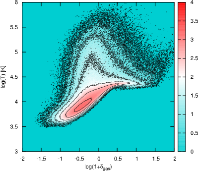
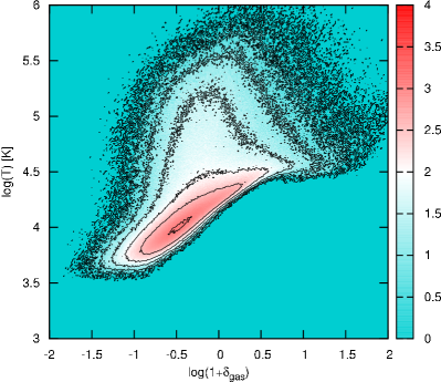
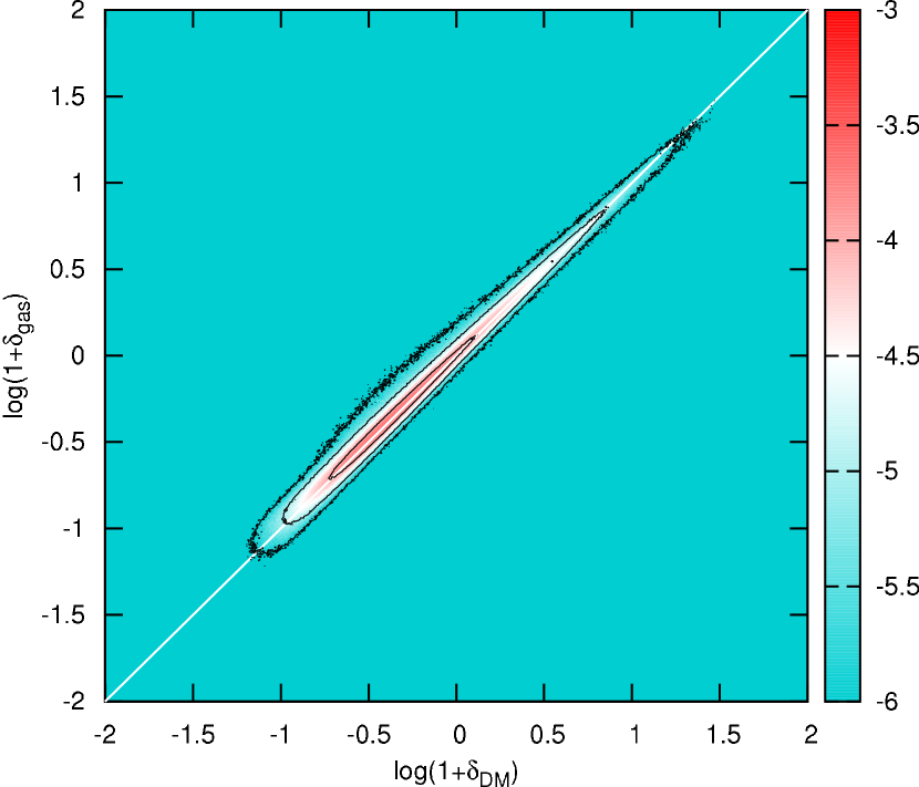
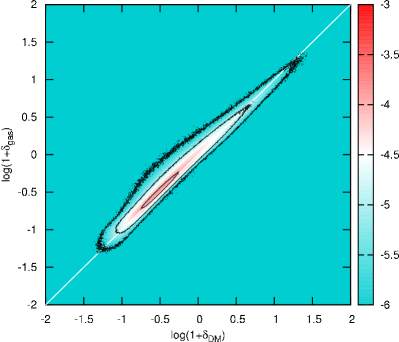
Figure 1: The top row shows the effective equation of state of a $12.5\;h^{-1}\textrm{ Mpc}$ gasdynamic simulation binned to cells of $80\;h^{-1}\textrm{ kpc}$ at redshift $z=5$ (left panels) and $z=4$ (right panels). The middle row shows the gas overdensity $1+\delta_{\mathrm{gas}}$ as a function of dark matter density $1+\delta_{\mathrm{DM}}$. The white diagonal line marks the linear relation if gas strictly follows the dark matter. In both rows the colour coding refers to the logarithm of the respective number of cells. The lowest row shows the probability distribution of the dark matter (solid line) and gas (dashed line) overdensity.

2.2 Model and calibration of the intergalactic medium

The characteristics of the IGM gas are determined analogously to the method described in P1. We will therefore only briefly sketch the method with which a representative IGM model is obtained.

The temperature in the IGM can be approximated by the so called effective equation of state (Hui & Gnedin, 1997), which is expressed as $T=T_{{\rm 0}}(1+\delta)^{\gamma-1}$. The effective equation of state shows a linear trend for overdensities $0.1\lesssim\delta\lesssim 10$ (compare Fig. 1). For higher densities its behaviour is approximated by assuming a constant value above a temperature cut-off $T_{\mathrm{cut-off}}=T\left(\delta=10\right)$. By employing the method developed in Hui et al. (1997), we compute H i Ly$\alpha$ absorption spectra from the DM density and velocity fields, once the parameters $T_{{\rm 0}}$, $\gamma$, and the UV background photoionisation rate ($\Gamma_{\rm UVB}$) are determined. These are constrained by matching statistical properties of the simulated H i absorption spectra with observed relations. Such a calibration will be important in obtaining realistic representations of the IGM that closely mimic the observed characteristics.

In order to calibrate our IGM model, we employ four observational constraints sorted by increasing importance: (i) The observed equation of state (Ricotti et al., 2000; Schaye et al., 2000; Lidz et al., 2010), (ii) the evolution of the UV background photoionisation rate (Haardt & Madau, 2001; Bianchi et al., 2001; Bolton et al., 2005; Dall’Aglio et al., 2008b, 2009), (iii) the observed evolution of the effective optical depth in the Ly$\alpha$ forest (Schaye et al., 2003; Kim et al., 2007), and (iv) the transmitted flux probability distribution (FPD, Becker et al., 2007).

The statistical quantities of the simulated spectra are derived from the simulation using 500 lines of sight randomly drawn through the cosmological box. Due to the availability of high resolution spectra with high signal-to-noise (S/N) ratios of up to 120, we approximate such high quality data by assuming noise free spectra. It has been noted by Calverley et al. (2011) that low S/N levels introduce a systematic shift in the proximity effect signal. Since we want to quantify the physical effect of the halo’s surrounding environment on UVB measurements, adding noise would only lead to degeneracies between the two effects. However we will briefly address the influence of noise in Section 4.2.

The spectra are convolved with the instrument profile of the UVES spectrograph and are then binned to the typical resolution of UVES spectra of $6.7\textrm{ km s}^{-1}$. We further assume that the QSO continuum can be perfectly determined and we therefore consider no uncertainties in the continuum. This procedure is adopted to precisely quantify physical effects without contamination of the signal with observational uncertainties. These will only increase the variance in the results discussed below.

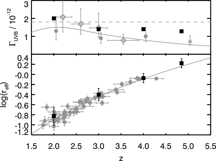
Figure 2: Upper panel: The evolution of the UV background photoionisation rate in the four snapshots (black squares) compared to Bolton et al. (2005) (grey points shifted by $\Delta z=0.05$ for better visibility), measurements by Dall’Aglio et al. (2008a) (grey open diamonds) and Calverley et al. (2011) (grey star), a fit to SDSS data measurements by Dall’Aglio et al. (2009) (grey dashed line) and predictions by Haardt & Madau (2001) (grey line). Lower panel: The effective optical depth of our models (black points) in comparison to measurements by Schaye et al. (2003) (grey points). The continuous line shows the fit to observational data by Kim et al. (2007).

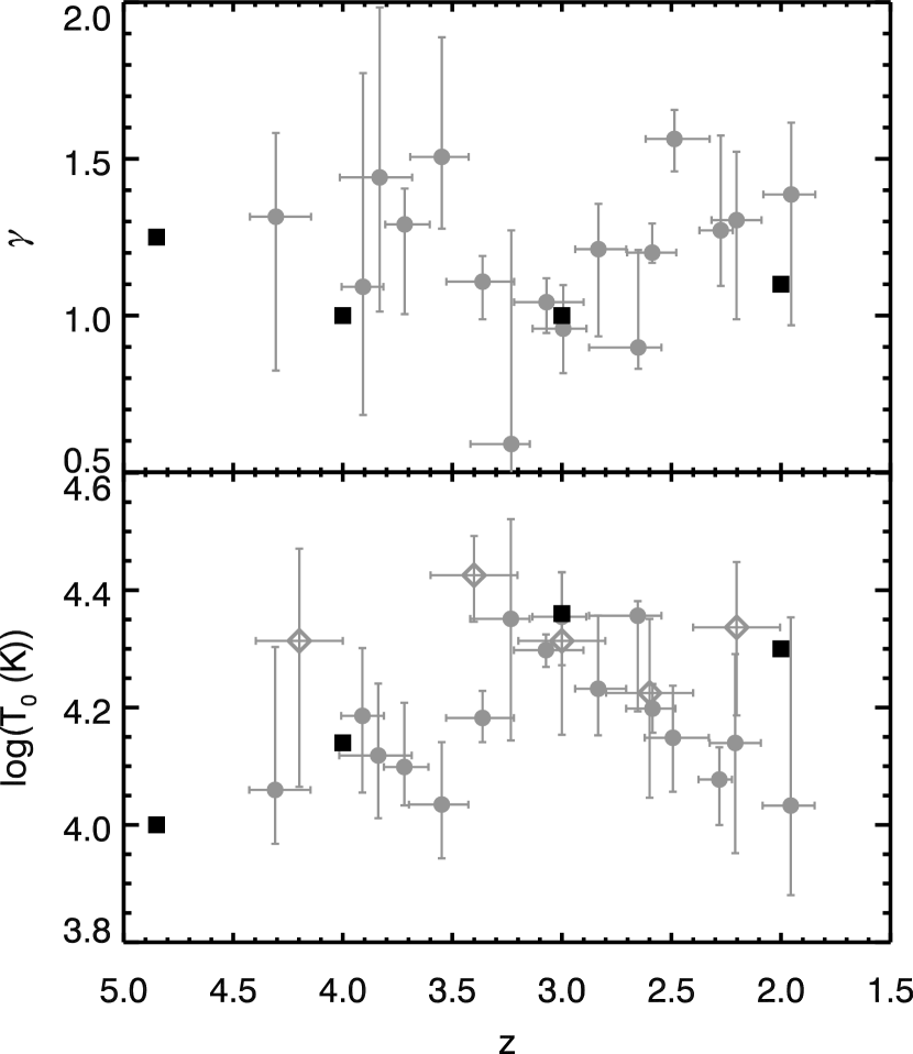
Figure 3: Upper panel: Comparison of our choices for $\gamma$ (black squares) with observationally derived results by Schaye et al. (2000) (grey points). Lower panel: Comparison of our model $T_{\rm 0}$ (black points) with observations by Schaye et al. (2000) (grey points) and Lidz et al. (2010) (grey open diamonds).

To determine the model parameters for the IGM, we adopt an iterative method based on $\chi^{2}$ minimisation between simulated and observed FPD, as the latter provides one of the strongest constrains on the Ly$\alpha$ forest properties. Our steps are as follows:

1. We choose a initial guess $\left(T_{{\rm 0}},\gamma,\Gamma_{\rm UVB}\right)_{0}$ according to the measurements of the equation of state by Schaye et al. (2000) and Lidz et al. (2010) and the evolution of the UVB by Haardt & Madau (2001) (see Figs. 2 and 3).

2. With the above initial guess and using 500 lines of sight, we determine the average effective optical depth $\tau_{\rm{eff}}(z)=-\ln\left\langle F(z)\right\rangle$ with $F$ being the transmitted flux and the averaging is performed over the whole line of sight. As $T_{{\rm 0}}$ and $\gamma$ have a subdominant effect on $\tau_{\rm{eff}}(z)$, we first tune $\Gamma_{\rm UVB}$ to obtain a match in the effective optical depths of the model spectra with recent observations from Kim et al. (2007). This results in a new set of parameters $\left(T_{{\rm 0}},\gamma,\Gamma_{\rm UVB}\right)_{1}$.

3. Finally we construct our simulated FPD. As observational constraint we employ the log normal fits obtained by Becker et al. (2007) in a redshift interval of $\Delta z=\pm 0.25$ centred on the snapshot redshift $z$ (see Fig. 4). By using their fits to the FPD, our model spectra can be compared with the observations without considering the effect of detector noise. However for consistency we also compare the simulated FPD with the raw combined observational results by Becker et al. (2007), folding the simulation result with the global noise function of the combined observed sample (see Fig. 5). The best fit parameters $\left(T_{{\rm 0}},\gamma,\Gamma_{\rm UVB}\right)_{\star}$ are then iteratively determined with a Simplex optimisation procedure.

Our best fit parameters are presented in Table 1, and plotted in Figs. 2, 3, 4, and 5 in comparison with different literature results.

Table 1: Model parameters of the semi-analytical model.

$z$	$\log(T_{0}[K])$	$\gamma$	$\Gamma_{\rm{UVB}}[\textrm{s}^{-1}]$	$\log\tau_{\mathrm{eff}}$
$4.8$	$4.00$	$1.25$	$1.16\times 10^{-12}$	$0.222$
$4.0$	$4.14$	$1.00$	$1.4\times 10^{-12}$	$-0.074$
$3.0$	$4.36$	$1.00$	$1.4\times 10^{-12}$	$-0.401$
$2.0$	$4.30$	$1.10$	$2.0\times 10^{-12}$	$-0.826$

The inferred evolution of the UV background in Fig. 2 closely follows recent results by Haardt & Madau (2001), Bolton et al. (2005), and Dall’Aglio et al. (2008b). The values for redshift $z=4.8$ is rather high when compared with Calverley et al. (2011), however it is still in agreement within the $2\sigma$ limits. Furthermore the effective optical depth, also shown in Fig. 2, is consistent with high resolution observations by Schaye et al. (2003) and Kim et al. (2007). Additionally the final parameters of the equation of state $T_{0}$ and $\gamma$ lie within the measurement uncertainties of Schaye et al. (2000) and Lidz et al. (2010), which is evident from Fig. 3.

The flux probability distributions estimated from the simulated sight lines agree reasonably well with the noise-corrected observed profiles estimated by Becker et al. (2007) who assumed a log-normal distribution of the optical depth in the Ly$\alpha$ forest (see Fig. 4). At redshifts $z=2\textrm{ and }3$ the match between the mean observed profiles and our simulations is good. However at higher redshifts, the agreement marginally decreases, even though the distributions are consistent within the variation between different lines of sight. This discrepancy manifests itself clearer when comparing the simulations with the raw observational data in Fig. 5 which include the effects of noise. The discrepancy is especially strong at the high transmission end of the distribution. This is most certainly caused by our crude noise modelling of a sample with inhomogeneous S/N, which we obtained by stacking the noise functions of the various lines of sight. On the other hand we assume a perfect knowledge of the continuum level in the spectra, which is a challenge to determine in observed spectra, especially at high redshifts.

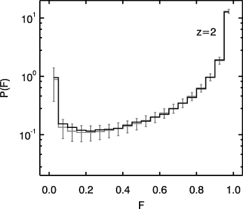
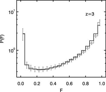
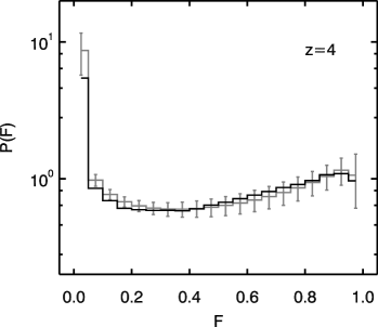
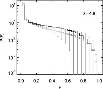
Figure 4: Probability distribution function of transmitted flux $F$ at redshifts 2, 3, 4, and 4.8. Grey lines give the mean observed PDF obtained from the fits excluding noise given in (Becker et al., 2007) with $1\sigma$ error bars denoting the variation between different lines of sight. The mean is derived in redshifts bins of $\pm 0.25$ centred on the model redshift. The black full line shows the results from our models.

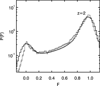
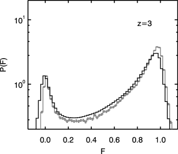
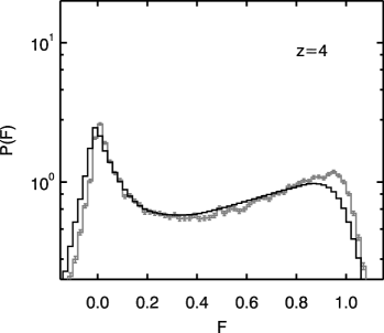
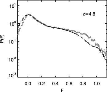
Figure 5: Probability distribution function of transmitted flux $F$ at redshifts 2, 3, 4, and 4.8. Grey lines with $1\sigma$ error bars give the observed PDF (Becker et al., 2007) and the black full line show the results obtained from our models folded with the signal to noise function of the combined observations. The combined observational data is derived in redshifts bins of $\pm 0.25$ centred on the model redshift.

3 Method

3.1 Line-of-sight proximity effect

Bright UV sources, such as QSOs, alter the ionisation state in their vicinity strongly up to proper distances of a couple of Mpc. The resulting change in the ionisation state directly translates into a decrease in optical depth. This decrease manifests itself in a reduction of the absorption line density in the Ly$\alpha$ forest when approaching the redshift of the source. Using line-counting statistics, Bajtlik et al. (1988) measured the line-of-sight proximity effect in QSO spectra for the first time. They assumed that QSOs are situated in a mean IGM environment, neglecting any redshift distortions from peculiar velocities of the absorption clouds. They further assumed that the QSO’s radiation field is radially decreasing from the source proportional to $r^{-2}$, i.e. geometric dilution. Using detailed radiative transfer simulations, P1 showed that radiative transfer effects only play a marginal role in the line-of-sight proximity effect and that the assumption of geometric dilution holds.

Assuming photoionisation equilibrium, the change in the optical depth as a function of distance $r$ to the QSO can be expressed as

$$\tau_{\mathrm{PE}}(r)=\tau_{\mathrm{Ly\alpha}}(r)\left(1+\omega(r)\right)^{-1}$$ (1)

(Liske & Williger, 2001), where $\tau_{\mathrm{PE}}$ is the observed optical depth, $\tau_{\mathrm{Ly\alpha}}$ is the optical depth in the absence of a QSO, and

$$\omega(r)=\frac{\Gamma_{\mathrm{QSO}}(r)}{\Gamma_{\mathrm{UVB}}}=\frac{1}{16\pi^{2}}\frac{1}{r^{2}}\frac{L_{\nu_{\mathrm{LL}}}}{J_{\nu_{\mathrm{LL}},\mathrm{UVB}}}\frac{3-\alpha_{\mathrm{b}}}{3-\alpha_{\mathrm{q}}}$$ (2)

acts as a normalised distance to the QSO (Dall’Aglio et al., 2008b). Here $\Gamma_{\mathrm{QSO}}(r)$ and $\Gamma_{\mathrm{UVB}}$ are the photoionisation rates of the QSO and the UV background respectively, $L_{\nu_{\mathrm{LL}}}$ is the QSO’s luminosity at the Lyman limit, while $J_{\nu_{\mathrm{LL}},\mathrm{UVB}}$ is the UVB’s Lyman limit flux, $\alpha_{\mathrm{b}}$ is the slope of the UVB’s spectral energy distribution $\propto\nu^{\alpha_{\mathrm{b}}}$, and $\alpha_{\mathrm{q}}$ denotes the spectral slope of the QSO’s emission $\propto\nu^{\alpha_{\mathrm{q}}}$. In this work we assume for simplicity the UVB to be dominated by QSOs. We therefore follow Haardt & Madau (1996) and chose the slope of the UVB to be $\alpha_{\mathrm{b}}=-1.5$. This is consistent with observations by Telfer et al. (2002) who find $\alpha_{\mathrm{q}}=-1.57\pm 0.17$. The effect of differing spectral shapes between the UVB and the QSO has been studied in Dall’Aglio et al. (2008b) and P1. The proximity effect is introduced into lines of sight drawn from our simulation boxes by modifying the neutral hydrogen fraction in real space using $n_{\mathrm{{\mathbf{H\,\text{{i}}}},PE}}(r)=n_{\mathrm{{\mathbf{H\,\text{{i}}}},Ly\alpha}}(r)\left(1+\omega(r)\right)^{-1}$.

3.2 Environments

To study the impact of the large scale environment on the proximity effect measurement as a function of QSO host halo mass, we pick halos in given mass ranges from the simulation to serve as QSO hosts. Around each halo, 100 lines of sight with a length of two comoving box sizes ($128\;h^{-1}\textrm{ Mpc}$) are randomly drawn from the box assuming periodic boundary conditions. Our sample of QSO host halos cover a wide range of masses. At each redshift we use the 20 most massive halos, 50 halos with a mass around $10^{12}M_{\astrosun}$, and 50 halos with a mass around $10^{11}M_{\astrosun}$. For the $10^{12}$ and $10^{11}M_{\astrosun}$ mass objects we choose 50 halos from the mass sorted halos with a mass larger than the cutoff. For the more massive bin, less than 50 halos with mass higher than the cutoff are present in the simulation at $z\geq 4$. In this case we choose all the halos above $10^{12}M_{\astrosun}$ and extend the range to lower masses until the sample consists of 50 halos. For these redshifts, the $10^{12}M_{\astrosun}$ mass range overlaps with the 20 most massive halos. The covered mass intervals are given in Table 2 as a function of redshift. We further note that the halos in the $10^{11}M_{\astrosun}$ mass bin are certainly not massive enough to host QSOs, since da Ângela et al. (2008) for instance estimated a QSO host halo mass of around $3\times 10^{12}M_{\astrosun}$ independent of redshift and luminosity from the 2dF-SDSS survey. However to establish any dependency of the proximity effect signal with the host’s mass, they are included for the purpose of an extreme low mass range.

Table 2: Mass range of the halo samples as a function of redshift. The $10^{12}\;M_{\astrosun}$ and $10^{11}\;M_{\astrosun}$ samples contain 50 halos each. The 20 most massive halos are given in units of $10^{12}\;M_{\astrosun}$, the other mass bins in units corresponding to the mass bin.

$z$	20 most massive	$10^{12}\;M_{\astrosun}$	$10^{11}\;M_{\astrosun}$
$4.8$	$2.07-0.92$	$2.07-0.53$	$1.04-1.00$
$4$	$4.84-1.51$	$4.84-0.88$	$1.03-1.00$
$3$	$15.8-3.41$	$1.38-1.00$	$1.01-1.00$
$2$	$40.2-6.19$	$1.14-1.00$	$1.01-1.00$

In order to test the influence of the large scale environment around QSO host halos we additionally construct a sample of lines of sight for each redshift where the origins are randomly selected. This sample provides a null hypothesis since any influence of large scale density fluctuations averages out if the origins of the lines of sight are randomly distributed in the box.

3.3 Measuring the proximity effect in spectra

The proximity effect signature is measured in Ly$\alpha$ forest spectra by first constructing an appropriate $\omega$-scale for the observed QSO. In this study we assume the QSO to have a Lyman limit luminosity of $L_{\nu_{\mathrm{LL}}}=10^{31}\textrm{ erg Hz}^{-1}\textrm{ s}^{-1}$, and the photoionisation rates of our model UVB field are used. We have shown in P1 that for higher QSO luminosities the proximity effect is more pronounced and less affected by the density distribution. Therefore we use a low luminosity QSO to obtain upper limits of the environmental bias. Given the $\omega$-scale, the transmission spectra is then evaluated for each line of sight in bins of $\Delta\log\omega$ (Dall’Aglio et al., 2008b). Using the mean transmission per bin, the effective optical depth in the bin $\tau_{\mathrm{eff,QSO}}(\Delta\log\omega)$ is calculated and normalised to the effective optical depth in the Ly$\alpha$ forest unaffected by the QSO’s radiation $\tau_{\mathrm{eff,Ly\alpha}}$. The normalised optical depth $\xi$ is thus

$$\xi(\Delta\log\omega)=\frac{\tau_{\mathrm{eff,QSO}}(\Delta\log\omega)}{\tau_{\mathrm{eff,Ly\alpha}}}.$$ (3)

The imprint of the proximity effect onto the normalised optical depth for a given $\omega$-scale becomes

$$\xi(\omega)=\left(1+\omega(r)\right)^{1-\beta}$$ (4)

(Liske & Williger, 2001) where $\beta$ is the slope of the Ly$\alpha$ absorber’s column density distribution. Throughout this work we assume $\beta=1.5$ (Kim et al., 2001). The UVB photoionisation rate $\Gamma_{\mathrm{UVB}}$ can then be determined using the proximity effect strength parameter $a$

$$\xi=\left(1+\frac{\omega}{a}\right)^{1-\beta}.$$ (5)

This parametrisation was introduced by (Dall’Aglio et al., 2008b, a) in analyses of observed spectra with an assumed UVB as reference. Values of $a>1$ or $a<1$ indicate a weaker or stronger proximity effect than the model, respectively. The measured photoionisation rate of the UVB is then determined using the reference value $\Gamma_{\mathrm{UVB,ref}}$ multiplied by the strength parameter $a$. In our case the strength parameter $a$ indicates any deviation of the measured UVB photoionisation rate from the input value. The strength parameter is determined by fitting Eq. 5 to the binned normalised optical depth $\xi(\Delta\log\omega)$. In order to exclude any direct impact of the host halo on the strength parameter fit, only data with $\log\omega<2$ have been used.

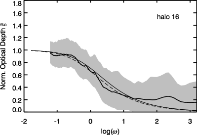
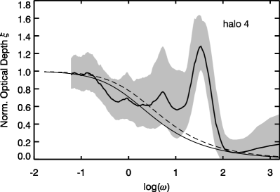
Figure 6: Mean normalised optical depth profiles obtained using a moving average smoothing with a kernel size of $\Delta\log(\omega)=0.5$ for two halos taken from the 20 most massive halo sample at redshift $z=4$ (black solid line with grey shading). The mean halo profiles are determined using 100 lines of sight and the shaded area gives the $1\sigma$ standard deviation. The analytical proximity effect model is given as the smooth black line, while the fitted profile is indicated by the dashed line. The left panel shows a halo without strong intervening density features and closely following the analytic model. The right panel illustrates a halo having strong density features in its vicinity, causing strong deviations from the analytical form.

In P1 we found the observed $\xi$ to fluctuate strongly around the analytical proximity effect profile. Any fit of Eq. 5 is thus biased by these large fluctuations which arise from the presence of strong absorbers along the line of sight.

In order to obtain a smoother $\xi$-profile, the wavelength scale of the spectrum is transformed into the $\log\omega$-scale and a boxcar smoothing (also known as moving average) with the size of $\Delta\log\omega$ is applied to the transmission spectrum. Analogously to the method given above, we then calculate the effective optical depth in each smoothed pixel and determine the normalised optical depth $\xi$. This results in smooth $\xi$-profiles allowing the identification of areas dominated by strong absorption systems.

In Fig. 6 two examples of mean $\xi$-profiles taken out of the 20 most massive halos sample at $z=4$ are given. A $\Delta\log\omega=0.5$ is found to yield a good balance between smoothing and retaining structure in the $\xi$-profile. For the mean $\xi$-profiles shown in Fig. 6, 100 lines of sight have been constructed randomly around the DM halos. The two examples illustrate a halo without any signs of intervening strong absorption systems (left panel) and one where a strong density feature is located near the host halo at $\log\omega=1.5$ (right panel). From the halo without strong nearby systems it becomes evident that the profile closely follows the analytical one. A fit to this smooth $\xi$-profile is now very robust, since the functional form of the profile is well constrained and the fit of Eq. 5 is not solely determined by a small number of data points. The same is true for cases with strong intervening absorption systems, as long as the underlying smooth profile of Eq. 4 is still visible. Strong deviations from the analytical form however, as presented in our second example, are large enough to prevent a clear identification of the smooth analytical profile and the obtained strength parameters have to be treated with caution.

4 Results

4.1 Null hypothesis: Random locations

In order to assess whether large scale over-densities affect the proximity effect profile and the associated strength parameter, we first establish results that are unaffected by such large scale density features. A sample of 500 randomly selected lines of sight originating at random points in the simulation will serve as a null hypothesis. No noise is added to the spectra. However we will use this sample in the next section to discuss the effect of detector noise on our results.

In Fig. 7 we discuss results obtained for redshifts $z=4.8,\textrm{ and }3$. For each line of sight, the normalised optical depth $\xi$ was calculated using the method described in Sect. 3.3. For each redshift we determine the mean and median $\xi$ profile, as well as the $\xi$ probability distribution as a function of $\omega$. The $\xi$ probability distribution is shown in colour coding in Fig. 7.

At $z=4.8$ the mean profile follows the analytic proximity effect model very well, with just a slight increase in its slope towards higher $\omega$ values. Note however that at large $\omega$ values of $\log\omega>2$, $\xi$ can only be poorly determined due to a very small number of pixels contributing to the $\Delta\omega$ bins. The median profile as well follows the input model up to $\log\omega\sim 0.5$. However at $\log\omega>0.5$ the median profile steepens strongly and starts to deviate from the input model and the mean profile. This indicates a growing asymmetry in the $\xi$ distribution with increasing $\omega$ (approaching the QSO), resulting in the growing discrepancy between the mean and median profiles. Considering the $\xi$ distribution function, the increasing skewness of the distribution becomes apparent. For $\log\omega<1$, the width of the distribution stays constant and appears symmetrical and normally distributed in the logarithmic scale. This indicates a log normal distribution of $\xi$ values. However at larger $\omega$ values the distribution starts to widen up and the peak in probability shifts towards lower values of $\log\xi$, moving away from the expectations of the analytical formalism.

For redshifts $z=4$ and $z=3$ a similar picture emerges. The $\xi$ distribution widens as a function of redshift, with an increase in its variance with decreasing redshift. The mean profile however always regains the input model well. However the discrepancy between the median profile and the mean at high $\omega$ values increases with decreasing redshift. The median profile becomes steeper and steeper, indicating a growing skewness of the $\xi$ distribution at high $\omega$. However at low $\omega$, the $\xi$ distribution stays symmetric and continues resembling a log normal distribution up to $\log\omega\sim 0$. At $z=2$, the $\xi$-distribution shows a strongly increasing variance, dominating over the signal of the input model completely. We will therefore not consider results from $z=2$ in this work.

The increase in variance is dominated by two factors. On the one hand the universe evolves and the growth of structure increases with decreasing redshift. This introduces stronger density contrasts between under- and overdense regions. On the other hand, the IGM becomes more transparent with decreasing redshift due to the increasing UV background and cosmic expansion reducing the mean density of the universe. Therefore at low redshifts, the Ly$\alpha$ forest traces denser structures than at high redshift.

From the simple test of this subsection we conclude that with randomly selected lines of sight of random origins, the input proximity effect model can be regained with the mean $\xi$ profile. In our sample this is valid for $z\geq 3$. The median profile however deviates more and more from the mean profile with decreasing redshift and cannot be used to measure the UV background from the proximity effect with the current analytical model, which is formulated for a mean IGM.

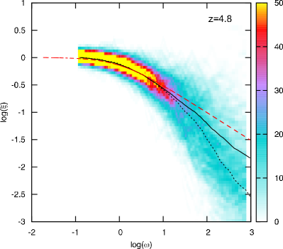
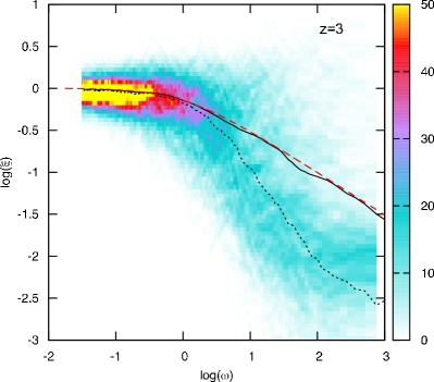
Figure 7: Frequency of the normalised optical depth $\xi$ using $\Delta\log\omega=0.5$ calculated from 500 random lines of sight drawn from our simulation box, as a function of $\omega$. The origins of these lines of sight were chosen not to be centred on any specific haloes, but on random points in the box. The left panel gives results for $z=4.8$ and the right panel $z=3$. The dashed line marks the input model used for generating the spectra including the proximity effect. The black solid line marks the mean $\xi$-profile, whereas the dotted black line marks the median profile.

Figure 8: The influence of the signal to noise ratio on the mean normalised optical depth $\xi$ for the null hypothesis. Shown are results at redshifts $z=4.8$ (left panel) and $z=3$ (right panel). The $\xi$-profiles have been normalised to results using a signal to noise of 150. The dotted line denotes a S/N of 10, the dashed line a S/N of 20, the dash dotted line a S/N of 50, and the dash triple dotted line a S/N of 100.

4.2 Dependence on the spectra signal to noise

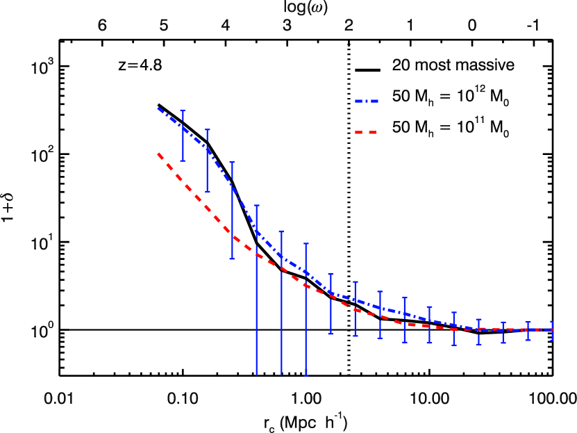
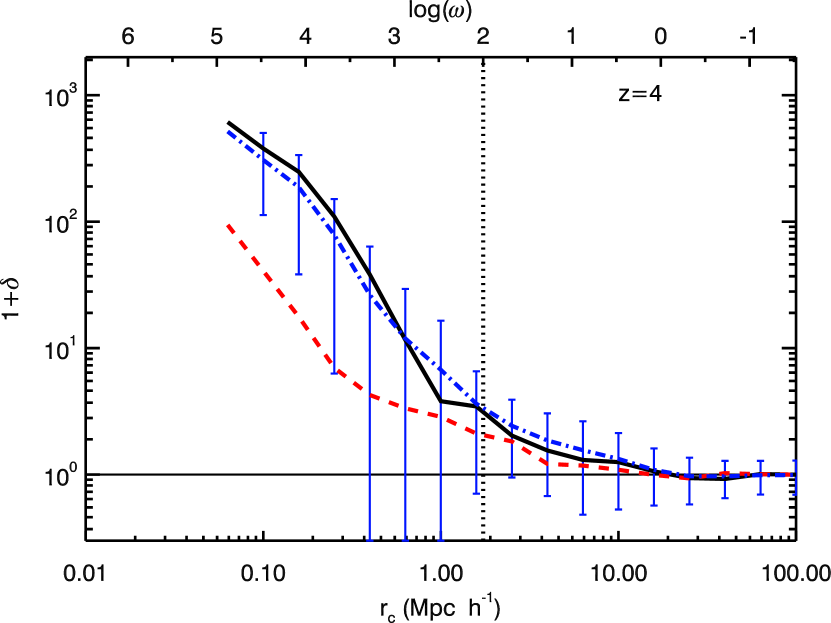
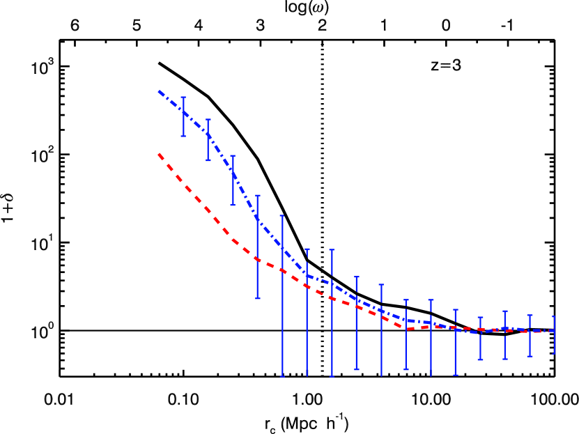
Figure 9: Mean density environment around all the halos in each mass bin. The density profiles are smoothed for better visibility. Further the corresponding $\omega$ scale is given as reference. The black solid line denotes the mean profile around the 20 most massive halos, the blue dash-dotted line denotes the mean around the $M_{\mathrm{halo}}=10^{12}\;M_{\astrosun}$ halos, and the red dashed line marks the mean around the $M_{\mathrm{halo}}=10^{11}\;M_{\astrosun}$ halos. The standard deviation is given for the $M_{\mathrm{halo}}=10^{12}\;M_{\astrosun}$ halos exemplary for the other environments. The first panel shows $z=4.8$, the second panel $z=4$, and the last panel $z=3$. The vertical dotted line marks the area of $\log\omega>2$ which was excluded in the determination of the strength parameter.

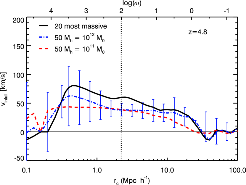
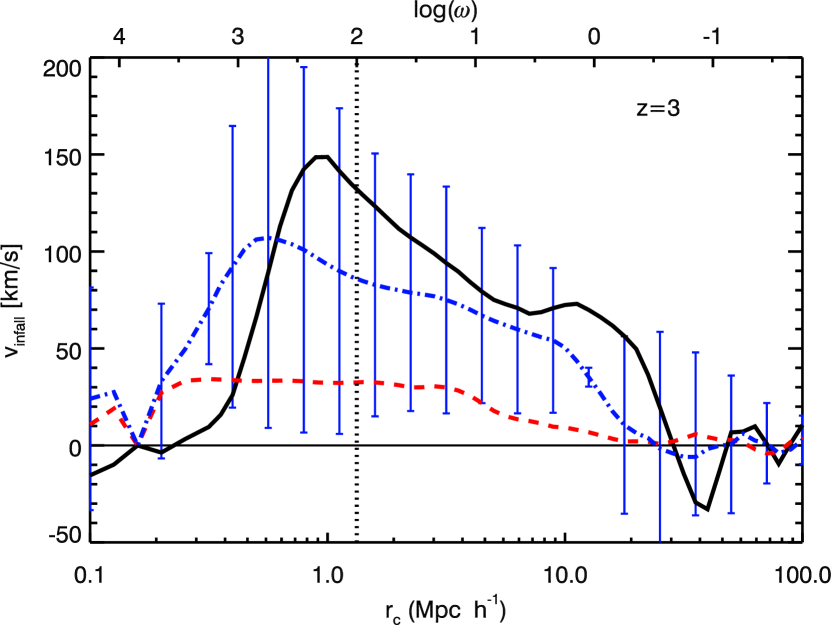
Figure 10: Mean infall velocity around all the halos in each mass bin. The infall velocity profiles are smoothed for better visibility. Further the corresponding $\omega$ scale is given as reference. The black solid line denotes the mean infall velocity around the 20 most massive halos, the blue dash-dotted line denotes the mean around the $M_{\mathrm{halo}}=10^{12}\;M_{\astrosun}$ halos, and the red dashed line marks the mean around the $M_{\mathrm{halo}}=10^{11}\;M_{\astrosun}$ halos. The standard deviation is given for the $M_{\mathrm{halo}}=10^{12}\;M_{\astrosun}$ halos exemplary for the other environments. The first panel shows $z=4.8$, the second panel $z=4$, and the last panel $z=3$. The vertical dotted line marks the area of $\log\omega>2$ which was excluded in the determination of the strength parameter.

We now want to discuss the effect of detector noise on the mean proximity effect profiles. Using the 500 lines of sight from the null hypothesis sample, noise is added to each spectrum using a signal to noise (S/N) of 10, 20, 50, 100, and 150. For each S/N sample we determine the mean $\xi$ profile and normalise it to the S/N$=150$ results. The influence of noise on the proximity effect signature is shown in Fig. 8, where the normalised $\xi$ profiles are shown for $z=4.8$ and $z=3$ as a function of the signal to noise.

The largest influence noise has on the profile is at high $\omega$ values where only a small number of pixels contribute to $\xi$. However for $\omega$ values below $\log\omega\sim 1.5$, the strong influence of the noise on the profile disappears. At $z=4.8$ an increase of noise effects can be noted at $\log\omega<0$. There the results with a S/N of 10 produce deviations of up to 5% from high signal to noise spectra. However already with a signal to noise of 50, the $\xi$ profile is regained with an accuracy of less than 1%. At $z=3$ convergence with the low noise results for $\log\omega<1.5$ is already achieved with a signal to noise of 20. In order to resolve the profile within 1% accuracy at higher $\omega$ values, a signal to noise of 50 is needed.

One has to keep in mind though that these results only apply to the combined sample and not to individual lines of sight. However this shows that with our approach of not considering noise in the spectra, high signal to noise results are very well approximated.

4.3 Large scale environment

We now want to characterise the large scale density and velocity environment around our QSO host halos. It has been shown by Prada et al. (2006) and Faucher-Giguère et al. (2008) that the mean density profile around massive halos does not reach the mean cosmic density before a halocentric distance of comoving $r_{c}\sim 10\;h^{-1}\textrm{ Mpc}$. For smaller radii the mean DM density around halos can be up to 10 times above the mean density for halocentric distances of comoving $r_{c}\sim 1\;h^{-1}\textrm{ Mpc}$. For even smaller radii the density profile is governed by the density profile of the host halo. A similar behaviour has been observed by P1. Faucher-Giguère et al. (2008) have further determined the bias caused by Doppler shifting of absorption lines due to infalling gas in proximity effect measurements. The additional bias is found to be similarly important to the effect of overdensities. This effect is naturally included in our synthetic spectra taken from the simulations.

These large scale features are caused by large scale modes perturbing the density distribution at scales of several Mpc. These large modes still experience linear growth and increase with decreasing redshifts. Since halos with very large masses form preferably where these large modes show a positive amplitude, an increase in density above the mean cosmic density is expected around very massive halos. Since low mass halos also form in regions where there is less power on large scales, the density profiles are expected to be less influenced.

In Fig. 9 the smoothed and radially averaged overdensity profiles of our halo sample are shown as a function of distance and halo mass. A consistent picture to previous findings emerges. At $z=4.8$ the profiles show a steep decline in density up to comoving distances of $r_{c}\sim 0.4\;h^{-1}\textrm{ Mpc}$ for the massive halos. This region directly shows the density profile of the host halo. For larger distances the slope with which the density decreases becomes shallower and a transition between the host halo profile and its surrounding density environment is seen. The profile then reaches the mean cosmic density at a distance above $r_{c}>10\;h^{-1}\textrm{ Mpc}$, independent of halo mass.

For $z=4$ the picture is similar, however differences between the low mass halos and the more massive ones increase. The most massive halos themselves now leave their imprint up to a radius of $r_{c}\sim 1\;h^{-1}\textrm{ Mpc}$, whereas the direct influence of the low mass host halos ends at $r_{c}\sim 0.3\;h^{-1}\textrm{ Mpc}$. The low mass halos show a less pronounced large scale overdensity with a shallower decline in density than the more massive halos. The transition point where the density profile reaches the mean cosmic density is again found at a radius of around $r_{c}\sim 10\;h^{-1}\textrm{ Mpc}$. Furthermore the large scale density around the halos shows slightly larger values than at $z=4.8$, which is due to the ongoing structure formation and the linear growth of the corresponding large wavelength modes.

At $z=3$ the differences between the various halo masses further increases. The transition point where the profile reaches the mean cosmic density starts to show a dependency on halo mass. The 20 most massive halos reach the mean density at a radius of $r_{c}>20\;h^{-1}\textrm{ Mpc}$, whereas the low mass halos already reach it at $r_{c}>7\;h^{-1}\textrm{ Mpc}$. Furthermore the large scale overdensity has grown in density. We therefore expect any influence of this large scale overdensity on the proximity effect measurement to increase with decreasing redshift. Additionally we do not expect a dependency of a possible bias with halo mass at high redshifts, since no large differences between the density profiles are seen. However at low redshifts, differences due to stronger large scale overdensities with increasing halo mass may leave an imprint in the proximity effect profile.

For completeness we show the mean infalling velocities as a function of distance to the host for each halo mass bin in Fig. 10. Analogously to the density environment, the infall velocities grow with decreasing redshift due to the onset of structure formation. The infall velocity profiles for the 20 most massive halos and the $M_{\mathrm{halo}}=10^{12}\;M_{\astrosun}$ sample behave similarly at all redshifts. Moving away from the halo, the infall velocity rises until it reaches its maximum at the position where the density profile shows a transition between the host halo and its surrounding density environment. At larger radii the infall velocity steadily decreases until no systematic infall towards the halo is seen anymore. The radii where the systematic infall vanishes is about the size of the large scale overdensity itself. In the case of the low mass halo though, the infall velocity remains constant at low velocities over the whole large scale overdensity.

4.4 Proximity effect strength as function of halo mass

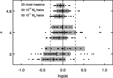
Figure 11: The $a$ parameter distribution as a function of halo mass and redshift. Each black dot represents the $a$ parameter obtained using the mean halo profile of 100 lines of sight. For each redshift the first line shows results from the 20 most massive halos sample, the second line represents the $M_{\mathrm{halo}}=10^{12}\;M_{\astrosun}$ sample, and the third line the $M_{\mathrm{halo}}=10^{11}\;M_{\astrosun}$ sample. The bold black lines indicate the sample’s mean $a$ parameter, while the grey shaded areas indicate the corresponding $1\sigma$ standard deviation. The solid line marks the fiducial model, while the dashed lines indicate deviations of a factor of two in the UVB measurements.

We now want to test whether the proximity effect strength parameter $a$ shows any dependency with the host halo mass. For each halo the mean $\xi$ profile is calculated from 100 lines of sight centred on the halo position. Then Eq. 5 is fitted to the mean profile and a proximity effect strength parameter $a$ is obtained for each halo in our sample. Any strength parameter with $\log a>0$ results in an overestimation of the UV background photoionisation rate in real measurements, whereas a $\log a<0$ resembles an underestimation.

In Fig. 11 each halo’s mean strength parameter $a$ is marked as a function of redshift and halo mass. The $a$ parameter distribution is thus obtained for each halo mass bin, and its mean and standard deviation are marked by the vertical bold line and grey area in the plot. At each redshift, the mean values of the distribution show no clear dependency with the host halo mass within the $1\sigma$ fluctuations. For redshift $z=4.8$, the different halo bins yield similar mean values and standard deviations. Considering the variance in the distribution, the input model is regained for all the halo mass bins at $z=4.8$.

This picture does not change with redshift. Against the expectations motivated by the overdensity profiles discussed in Sect. 4.3, the data shows no dependency on the halo mass. Even at $z=3$, where the mean large scale overdensity was found to be lower around lower mass halos than around high mass ones, no significant dependency is seen. The mean values are thus consistent with the input model within $1\sigma$. The halo to halo variance increases with decreasing redshift and the strength parameter distribution broadens. At $z=4.8$ the standard deviation of the whole halo sample is $\sigma(\log a)=0.08$, while at $z=4$ we find $\sigma(\log a)=0.20$ and $\sigma(\log a)=0.36$ for $z=3$. A similar increase in the variance has been previously observed by Dall’Aglio et al. (2008a) for individual lines of sight of a high-resolution QSO sample.

From these results we conclude that the proximity effect measurements do not show any host halo mass dependent bias. The variance in the signal between different halos increases with decreasing redshift and tighter constraints are obtained with higher redshift objects. However even at low redshifts, the mean strength parameter regained the input value within a factor of less than two.

4.5 Influence of the large scale overdensity

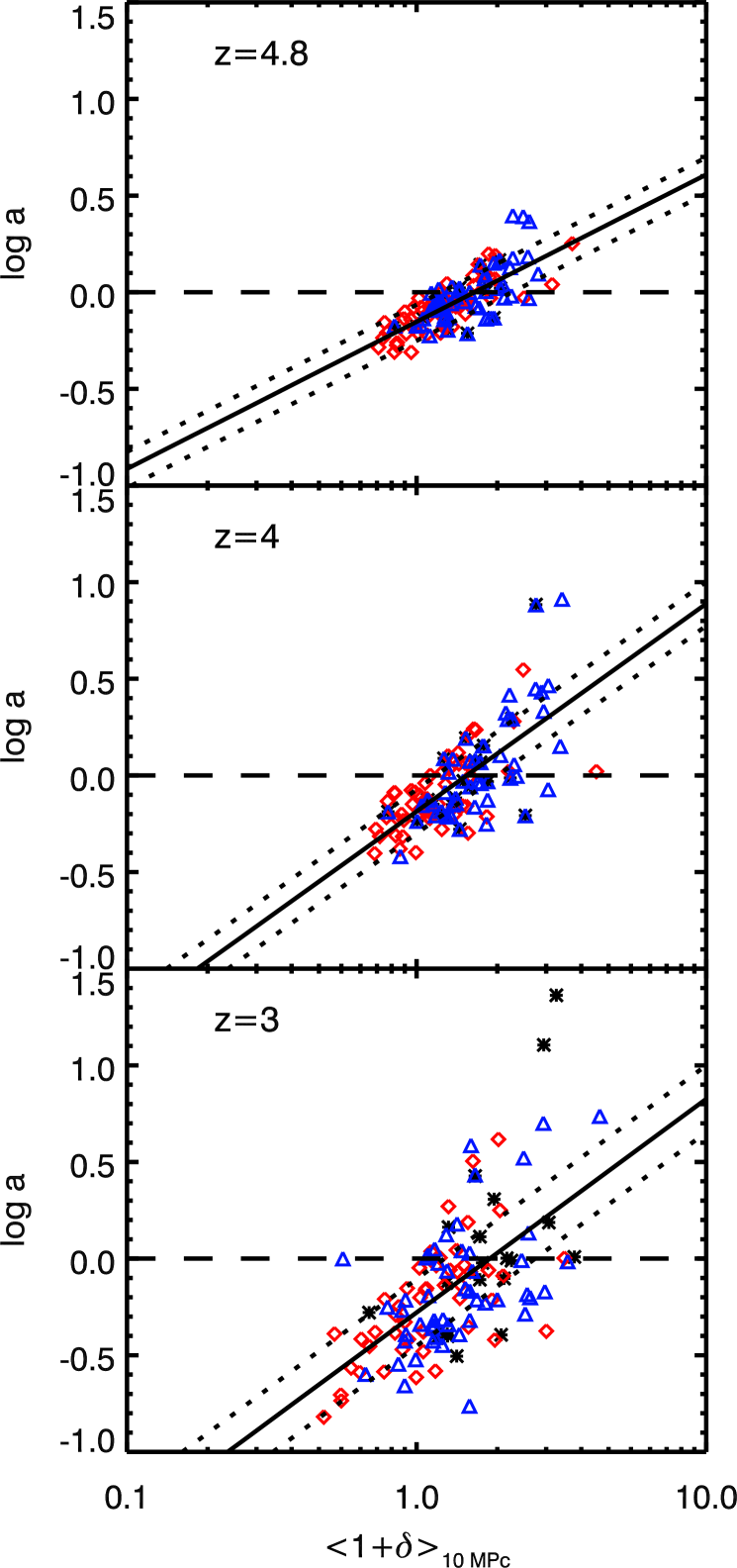
Figure 12: Proximity effect strength parameter as a function of the mean overdensity in a shell of $1$ to $10\;h^{-1}\textrm{ Mpc}^{-1}$ comoving radius around the 20 most massive halos (black asterisks), $M_{\mathrm{halo}}=10^{12}\;M_{\astrosun}$ halos (blue triangles), and $M_{\mathrm{halo}}=10^{11}\;M_{\astrosun}$ halos (red diamonds). The black dashed line marks $a=1$. The solid line represent linear regressions obtained from the dataset where the dotted lines mark the $1\sigma$ upper and lower boundaries.

In the previous section we have shown that the proximity effect strength parameter is not affected by the host halo mass. However a large scatter around the mean strength parameter is seen in each mass bin, which increases with decreasing redshift. We now want to establish the physical cause of the scatter, and therefore check if this scatter is connected with the density enhancement seen on large scales of up to comoving radii of $r_{c}=10\;h^{-1}\textrm{ Mpc}$.

For each halo, the mean overdensity profile is calculated using the density distribution along each line of sight. Then the mean over-density $\left<\delta\right>_{R}$ between the radii $r_{\mathrm{1}}$ and $r_{\mathrm{2}}$ is calculated from the mean density distribution around the halo using

$$\left<\delta\right>_{R}=\frac{1}{r_{\mathrm{2}}-r_{\mathrm{1}}}\int_{r_{\mathrm{1}}}^{r_{\mathrm{2}}}\delta(r)\;\mathrm{d}r.$$ (6)

We choose $r_{\mathrm{1}}=1\;h^{-1}\textrm{ Mpc}$ comoving in order to exclude the influence of the host halo on the density profile, since we are only interested in the large scale density distribution. The integral extends to comoving $r_{\mathrm{2}}=10\;h^{-1}\textrm{ Mpc}$ which is the characteristic size of the large scale density enhancements (see Sect. 4.3).

In Fig. 12 the strength parameter $a$ is correlated with the mean overdensity in the comoving radial interval $r_{c}=[1,\;10]\;h^{-1}\textrm{ Mpc}$. The various symbols indicate the different halo mass samples. At all redshifts, a correlation between the mean density in the vicinity of the QSO and the strength parameter of the mean $\xi$-profile is seen. A linear regression $\log a=\log\left<1+\delta\right>_{0}+\alpha\log\left<1+\delta\right>_{\mathrm{10Mpc}}$ is derived from the data, where $\log\left<1+\delta\right>_{0}$ is the normalisation point and $\alpha$ is the slope of the regression. The resulting fit parameters are listed in Table 3 together with the Pearson product-moment correlation coefficient $r$ of the data set.

Table 3: Table of linear regression results of the overdensity-strength parameter relation, together with the data’s Pearson product-moment correlation coefficients $r$. The uncertainties in the fitting parameters have been determined with the bootstrap technique.

$z$	$\log\left<1+\delta\right>_{0}$	$\alpha$	$r_{\mathrm{Pearson}}$
$4.8$	$-0.15\pm 0.07$	$0.76\pm 0.08$	$0.74$
$4.0$	$-0.19\pm 0.13$	$1.07\pm 0.16$	$0.68$
$3.0$	$-0.28\pm 0.19$	$1.11\pm 0.17$	$0.60$

Looking at the $z=4.8$ results, the data points align clearly on a power law relation. With a Pearson correlation coefficient of $r_{\mathrm{Pearson}}=0.74$ the data exhibits a tight correlation between the two quantities. The higher the mean density around a halo becomes, the stronger the proximity effect is biased towards larger strength parameters. At $z=4.8$ a strength parameter of $a=1$ (resembling an unbiased measurement of the photoionisation rate) is obtained for a mean overdensity of $\left<1+\delta\right>_{10\mathrm{Mpc}}\sim 1.6\pm 0.35$. It is interesting to note that there is no strong segregation between the various halo mass bins along the density axis. However, the lower mass halos lie to slightly lower overdensities than the more massive ones. All the different mass bins cover a similar range of large scale densities. Again this indicates that there is no distinct connection between the halo mass and the mean overdensity on these large scales. Hence, only the amount of matter in the greater vicinity of a halo is responsible for the large scatter in the strength parameter $a$ seen in the previous section. However, a small scatter in $a$ of $\approx 20\%$ around the linear regression remains at $z=4.8$.

Similar findings apply to the lower redshift results. The $a$ parameters are still related through a power law with the large scale overdensity, however the strength of the correlation drops to $r_{\mathrm{Pearson}}=0.60$ at $z=3$. Comparing the $z=4.8$ results with the lower redshift ones shows a slight steepening of the relation from $\alpha=0.76\pm 0.08$ at $z=4.8$ to $\alpha=1.11\pm 0.17$ at $z=3$. The scatter around the power law increases to $\approx 35\%$ for $z=4$ and 55% for $z=3$. Further the scatter seems to spread with increasing density, however a larger halo sample from a larger simulation would be needed to conclusively determine this increase in the variance. Again no bias in the strength parameter is found for an overdensity of $\left<1+\delta\right>_{10\mathrm{Mpc}}\sim 1.5\pm 0.52$ at $z=4$ and $\left<1+\delta\right>_{10\mathrm{Mpc}}\sim 1.8\pm 0.77$ at $z=3$.

These results show that the large scale distribution of matter around a host halo affects the proximity effect strength parameter and biases the measurements of the UV background photoionisation rate. There is a power law correlation between the mean density surrounding a QSO host and the $a$ parameter. The bias on the UV background photoionisation rate can be determined, if the mean overdensity around a QSO is inferred. However, density measurements from the Ly$\alpha$ forest are degenerated with the UV background photoionisation rate. The properties of the UV background have to be known in order to convert optical depths into densities.

Observationally, D’Odorico et al. (2008) have shown that QSOs at $z=2.6$ are situated in regions showing a density excess on scales of 4 proper Mpc. Due to the dependency of the results on the UV background photoionisation rate, their results only constrain the mean density of the large scale overdensity to a factor of about 3. Nevertheless we estimate a mean density in a radius of 4 proper Mpc from their results. We obtain an upper value on the mean overdensity of $\left<1+\delta\right>\sim 3.5$ and a lower value of $\left<1+\delta\right>\sim 1.25$. According to our results at $z=3$, this would translate into a bias of the strength parameter of $a=2.1$ for an overdensity of $3.5$ and $a=0.7$ for the lower value on the mean density around a QSO. Remember though that our results only apply to a QSO with a Lyman limit luminosity of $L_{\nu_{\mathrm{LL}}}=10^{31}\textrm{ erg Hz}^{-1}\textrm{ s}^{-1}$. According to P1 the bias becomes smaller for higher luminosity QSOs.

5 Conclusion

We have studied the effect of the host halo mass and the large scale density distribution on measurements of the proximity effect strength parameter. The strength parameter is observationally used to infer the UV background photoionisation rate. From a $64\;h^{-1}\textrm{ Mpc}$ sized dark-matter simulation, we picked the 20 most massive halos, 50 halos with a mass around $M_{\mathrm{halo}}=10^{12}\;M_{\astrosun}$, and another 50 halos with a mass around $M_{\mathrm{halo}}=10^{11}\;M_{\astrosun}$ at redshifts $z=4.8,\,4,\textrm{ and }3$. Each halo is individually assumed to host a QSO with a Lyman limit luminosity of $L_{\nu_{\mathrm{LL}}}=10^{31}\textrm{ erg Hz}^{-1}\textrm{ s}^{-1}$.

Around each halo, 100 random lines of sight of the density and velocity distribution are obtained. Using models of the IGM which we calibrated to observational constraints, the neutral hydrogen fractions and gas temperatures along each line of sight are inferred. To include the increase in ionisation of an additional QSO radiation field, the neutral hydrogen fractions are decreased proportional to geometric dilution of the QSO flux field (Partl et al., 2010). Then, for each line of sight, a Ly$\alpha$ forest spectrum is computed. From the spectrum we derive the mean proximity effect signature with observational methods and measure the proximity effect strength parameter $a$. Since the UV background photoionisation rate used in generating the Ly$\alpha$ spectra is known, the strength parameter quantifies the over- or underestimation of the UV background.

In order to assess whether the QSO host environment affects the proximity effect signal, a null hypothesis test was performed. From the simulation box, 500 lines of sight originating at random positions with random directions have been obtained. On each line of sight, the proximity effect was modelled. From these lines of sight, we obtained the distribution of normalised optical depths $\xi$ as a function of normalised distance to the QSO $\omega$. From the $\xi$-distribution, the mean and median proximity effect signals were determined. The mean profiles match the analytic model very well and the model UV photoionisation rates are regained. At large halocentric distances, the median and the mean profiles match. However the median increasingly deviates from the analytic model and the mean profile with decreasing distance to the QSO. This indicates that the $\xi$-distribution closely resembles a log normal distribution at large distances from the QSO, however it is increasingly skewed when nearing the source. Not only is the variance of the $\xi$-distribution found to increase with decreasing redshift, but its skewness increases as well.

We further determined the mean density distribution and infall velocity around all the halos in each mass bin as a function of redshift. For all redshifts the density profile does not immediately reach the mean cosmic density at the border of the dark matter halo, however it stays above the mean density up to comoving halocentric radii of $r_{c}\gtrsim 10\;h^{-1}\textrm{ Mpc}$. For redshifts $z=4.8$ and $z=4$ the size of this large scale overdensity is independent of the halo mass. However higher mass halos show in the mean a larger overdensity than lower mass halos. At redshift $z=3$ the size of the large scale overdensity is smaller for the lower mass sample than for the more massive ones. The velocity field shows a mean infall up to distances of $30\;h^{-1}\textrm{ Mpc}$ around the halos, reaching for the most massive halos $80$, $100$, and $150\textrm{ km/s}$ for redshifts $z=4.8,\;4,$ and $3$, respectively. Overdensity and infall velocities act together in the derived bias of the proximity effect.

The mean strength parameter per halo mass bin does not show a dependency with the halo mass. For each halo mass bin, a mean strength parameter which is consistent with the input model is regained within $1\sigma$ standard deviation. However the halo to halo variance is found to increase with decreasing redshift from $\sigma(\log a)=0.08$ at $z=4.8$ to $\sigma(\log a)=0.36$ at $z=3$.

The strength parameter is found to correlate with the mean density measured in a shell of comoving $1-10\;h^{-1}\textrm{ Mpc}$. We fit a power law to this correlation. Regions with a mean density below the cosmic mean show a stronger proximity effect than regions with densities above the cosmic mean. The correlation is tightest at $z=4.8$ and the scatter around the power law increases with decreasing redshift. Furthermore, the power law is found to steepen slightly with decreasing redshift. From these results we find that an unbiased UV background photoionisation rate can only be obtained if the mean density around the QSO is between $\left<1+\delta\right>_{10\mathrm{Mpc}}\sim 1.5\pm 0.52$ and $1.8\pm 0.77$.

If a possibility exists to determine the mean density around a QSO, the bias arising from the large scale overdensity can be corrected for. However density measurements from Ly$\alpha$ forest spectra are degenerate with the UV background photoionisation rate. Due to this degeneracy, previous measurements of the density distribution around QSOs, such as D’Odorico et al. (2008), have only been able to constrain the mean density up to a factor of 3. By inferring the bias of the proximity effect at $z\sim 3$ according to their density measurements, the strength parameter ranges from $a=0.7$ to $a=2.1$ for a QSO with a Lyman limit luminosity of $L_{\nu_{\mathrm{LL}}}=10^{31}\textrm{ erg Hz}^{-1}\textrm{ s}^{-1}$.

References

- Bajtlik et al. (1988) Bajtlik S., Duncan R. C., Ostriker J. P., 1988, ApJ, 327, 570
- Becker et al. (2007) Becker G. D., Rauch M., Sargent W. L. W., 2007, ApJ, 662, 72
- Bianchi et al. (2001) Bianchi S., Cristiani S., Kim T.-S., 2001, A&A, 376, 1
- Bolton & Haehnelt (2007) Bolton J. S., Haehnelt M. G., 2007, MNRAS, 382, 325
- Bolton et al. (2005) Bolton J. S., Haehnelt M. G., Viel M., Springel V., 2005, MNRAS, 357, 1178
- Calverley et al. (2011) Calverley A. P., Becker G. D., Haehnelt M. G., Bolton J. S., 2011, MNRAS, 412, 2543
- Carswell et al. (1982) Carswell R. F., Whelan J. A. J., Smith M. G., Boksenberg A., Tytler D., 1982, MNRAS, 198, 91
- Cooke et al. (1997) Cooke A. J., Espey B., Carswell R. F., 1997, MNRAS, 284, 552
- Cristiani et al. (1995) Cristiani S., D’Odorico S., Fontana A., Giallongo E., Savaglio S., 1995, MNRAS, 273, 1016
- da Ângela et al. (2008) da Ângela J., Shanks T., Croom S. M., Weilbacher P., Brunner R. J., Couch W. J., Miller L., Myers A. D., Nichol R. C., Pimbblet K. A., de Propris R., Richards G. T., Ross N. P., Schneider D. P., Wake D., 2008, MNRAS, 383, 565
- Dall’Aglio et al. (2008a) Dall’Aglio A., Wisotzki L., Worseck G., 2008a, A&A, 491, 465
- Dall’Aglio et al. (2008b) Dall’Aglio A., Wisotzki L., Worseck G., 2008b, A&A, 480, 359
- Dall’Aglio et al. (2009) Dall’Aglio A., Wisotzki L., Worseck G., 2009, ArXiv e-prints, arxiv:0906.1484
- D’Odorico et al. (2008) D’Odorico V., Bruscoli M., Saitta F., Fontanot F., Viel M., Cristiani S., Monaco P., 2008, MNRAS, 389, 1727
- Faucher-Giguère et al. (2008) Faucher-Giguère C., Lidz A., Hernquist L., Zaldarriaga M., 2008, ApJ, 688, 85
- Faucher-Giguère et al. (2008) Faucher-Giguère C.-A., Lidz A., Zaldarriaga M., Hernquist L., 2008, ApJ, 673, 39
- Giallongo et al. (1996) Giallongo E., Cristiani S., D’Odorico S., Fontana A., Savaglio S., 1996, ApJ, 466, 46
- Gottlöber et al. (2010) Gottlöber S., Hoffman Y., Yepes G., 2010, in Wagner S., Steinmetz M., Bode A., Müller M., eds, Proceedings of ”High Performance Computing in Science and Engineering” Vol. arxiv:1005.2687, Constrained Local UniversE Simulations (CLUES). Springer-Verlag, p. 309
- Guimarães et al. (2007) Guimarães R., Petitjean P., Rollinde E., de Carvalho R. R., Djorgovski S. G., Srianand R., Aghaee A., Castro S., 2007, MNRAS, 377, 657
- Haardt & Madau (1996) Haardt F., Madau P., 1996, ApJ, 461, 20
- Haardt & Madau (2001) Haardt F., Madau P., 2001, in Neumann D. M., Tran J. T. V., eds, Clusters of Galaxies and the High Redshift Universe Observed in X-rays Modelling the UV/X-ray cosmic background with CUBA
- Haardt & Madau (2011) Haardt F., Madau P., 2011, ArXiv e-prints, arxiv:1103.5226
- Hinshaw et al. (2009) Hinshaw G., Weiland J. L., Hill R. S., Odegard N., Larson D., Bennett C. L., Dunkley J., Gold B., Greason M. R., Jarosik N., KomatsuE. Nolta M. R., Page L., Spergel D. N., Wollack E., Halpern M., Kogut A., Limon M., Meyer S. S., 2009, ApJS, 180, 225
- Hui & Gnedin (1997) Hui L., Gnedin N. Y., 1997, MNRAS, 292, 27
- Hui et al. (1997) Hui L., Gnedin N. Y., Zhang Y., 1997, ApJ, 486, 599
- Jena et al. (2005) Jena T., Norman M. L., Tytler D., Kirkman D., Suzuki N., Chapman A., Melis C., Paschos P., O’Shea B., So G., Lubin D., Lin W., Reimers D., Janknecht E., Fechner C., 2005, MNRAS, 361, 70
- Kim et al. (2007) Kim T.-S., Bolton J. S., Viel M., Haehnelt M. G., Carswell R. F., 2007, MNRAS, 382, 1657
- Kim et al. (2001) Kim T.-S., Cristiani S., D’Odorico S., 2001, A&A, 373, 757
- Kirkman et al. (2005) Kirkman D., Tytler D., Suzuki N., Melis C., Hollywood S., James K., So G., Lubin D., Jena T., Norman M. L., Paschos P., 2005, MNRAS, 360, 1373
- Klypin et al. (1999) Klypin A., Gottlöber S., Kravtsov A. V., Khokhlov A. M., 1999, ApJ, 516, 530
- Lidz et al. (2010) Lidz A., Faucher-Giguère C., Dall’Aglio A., McQuinn M., Fechner C., Zaldarriaga M., Hernquist L., Dutta S., 2010, ApJ, 718, 199
- Liske & Williger (2001) Liske J., Williger G. M., 2001, MNRAS, 328, 653
- Loeb & Eisenstein (1995) Loeb A., Eisenstein D. J., 1995, ApJ, 448, 17
- Lu et al. (1991) Lu L., Wolfe A. M., Turnshek D. A., 1991, ApJ, 367, 19
- McDonald & Miralda-Escudé (2001) McDonald P., Miralda-Escudé J., 2001, ApJ, 549, L11
- Meiksin & White (2001) Meiksin A., White M., 2001, MNRAS, 324, 141
- Meiksin & White (2003) Meiksin A., White M., 2003, MNRAS, 342, 1205
- Meiksin (2009) Meiksin A. A., 2009, Reviews of Modern Physics, 81, 1405
- Miralda-Escudé et al. (1996) Miralda-Escudé J., Cen R., Ostriker J. P., Rauch M., 1996, ApJ, 471, 582
- Murdoch et al. (1986) Murdoch H. S., Hunstead R. W., Pettini M., Blades J. C., 1986, ApJ, 309, 19
- Partl et al. (2010) Partl A. M., Dall’Aglio A., Müller V., Hensler G., 2010, A&A, 524, A85+
- Petitjean et al. (1995) Petitjean P., Mücket J. P., Kates R. E., 1995, A&A, 295, L9
- Prada et al. (2006) Prada F., Klypin A. A., Simonneau E., Betancort-Rijo J., Patiri S., Gottlöber S., Sanchez-Conde M. A., 2006, ApJ, 645, 1001
- Rauch et al. (1997) Rauch M., Miralda-Escude J., Sargent W. L. W., Barlow T. A., Weinberg D. H., Hernquist L., Katz N., Cen R., Ostriker J. P., 1997, ApJ, 489, 7
- Ricotti et al. (2000) Ricotti M., Gnedin N. Y., Shull J. M., 2000, ApJ, 534, 41
- Rollinde et al. (2005) Rollinde E., Srianand R., Theuns T., Petitjean P., Chand H., 2005, MNRAS, 361, 1015
- Schaye et al. (2003) Schaye J., Aguirre A., Kim T.-S., Theuns T., Rauch M., Sargent W. L. W., 2003, ApJ, 596, 768
- Schaye et al. (2000) Schaye J., Theuns T., Rauch M., Efstathiou G., Sargent W. L. W., 2000, MNRAS, 318, 817
- Scott et al. (2000) Scott J., Bechtold J., Dobrzycki A., Kulkarni V. P., 2000, ApJS, 130, 67
- Songaila et al. (1999) Songaila A., Hu E. M., Cowie L. L., McMahon R. G., 1999, ApJ, 525, L5
- Springel (2005) Springel V., 2005, MNRAS, 364, 1105
- Springel & Hernquist (2003) Springel V., Hernquist L., 2003, MNRAS, 339, 289
- Srianand & Khare (1996) Srianand R., Khare P., 1996, MNRAS, 280, 767
- Telfer et al. (2002) Telfer R. C., Zheng W., Kriss G. A., Davidsen A. F., 2002, ApJ, 565, 773
- Theuns et al. (1998) Theuns T., Leonard A., Efstathiou G., Pearce F. R., Thomas P. A., 1998, MNRAS, 301, 478
- Tytler (1987) Tytler D., 1987, ApJ, 321, 69
- Tytler et al. (2004) Tytler D., Kirkman D., O’Meara J. M., Suzuki N., Orin A., Lubin D., Paschos P., Jena T., Lin W., Norman M. L., Meiksin A., 2004, ApJ, 617, 1
- Williger et al. (1994) Williger G. M., Baldwin J. A., Carswell R. F., Cooke A. J., Hazard C., Irwin M. J., McMahon R. G., Storrie-Lombardi L. J., 1994, ApJ, 428, 574