Farey Graphs as Models for Complex Networks

Abstract

Farey sequences of irreducible fractions between 0 and 1 can be related to graph constructions known as Farey graphs. These graphs were first introduced by Matula and Kornerup in 1979 and further studied by Colbourn in 1982 and they have many interesting properties: they are minimally 3-colorable, uniquely Hamiltonian, maximally outerplanar and perfect. In this paper we introduce a simple generation method for a Farey graph family, and we study analytically relevant topological properties: order, size, degree distribution and correlation, clustering, transitivity, diameter and average distance. We show that the graphs are a good model for networks associated with some complex systems.

1 Introduction

A Farey sequence of order $n$ is the sorted sequence of irreducible fractions between $0$ and $1$ with denominators less than or equal to $n$ and arranged in increasing values. Therefore, each Farey sequence starts with $0$ and ends with $1$, denoted by $\frac{0}{1}$ and $\frac{1}{1}$, respectively. The Farey sequences of orders 1 to 4 are: $F_{1}=\{{0\over 1},{1\over 1}\}$, $F_{2}=\{{0\over 1},{1\over 2},{1\over 1}\}$, $F_{3}=\{{0\over 1},{1\over 3},{1\over 2},{2\over 3},{1\over 1}\}$, $F_{4}=\{{0\over 1},{1\over 4},{1\over 3},{1\over 2},{2\over 3},{3\over 4},{1\over 1}\}$.

Farey sequences, which in some papers are incorrectly called Farey series, can be constructed using mediants (the mediant of $a\over b$ and $c\over d$ is ${a+c}\over{b+d}$): the Farey sequence of order $n$ is obtained from the Farey sequence of order $n-1$ by computing the mediant of each two consecutive values in the Farey sequence of order $n-1$, keeping only the subset of mediants that have denominator $n$, and placing each mediant between the two values from which it was computed. Note that neighboring fractions in a sequence are unimodular, i.e. if $p/q$ and $r/s$ are neighboring fractions, then $rq-ps=1$. It was John Farey who in 1816 conjectured that new terms in $F_{n}$ could be obtained as mediants from two consecutive terms in $F_{n-1}$. Cauchy proved the conjecture and used the term Farey sequences for the first time. However, Farey sequences were in fact introduced in 1802 by C. Haros, see [16].

Farey sequences have many interesting properties, which we will not review here and we refer the interested reader to the abundant literature on this topic, see [30] and references therein. As we are interested in some connections of these sequences with graph theory, we first mention their relation with Farey trees (which some authors call Farey graphs, but are a different structure than the graphs studied in this paper). A Farey tree is a binary tree labeled in terms of a Farey sequence and it is constructed as follows: The left child of any number is its mediant with the nearest smaller ancestor, and the right child is the mediant with its nearest larger ancestor. Using 2/3 as an example, its closest smaller ancestor is 1/2, so the left child is 3/5, and its closest larger ancestor is 1/1, and the right child is 3/4. The process can continue indefinitely, see Fig. 1. Note that on each level the numbers appear always in order and that all the rationals within the interval [0,1] are included in the infinite Farey tree. Moreover, the Farey sequence of order $n$ may be found by an inorder traversal of this tree, backtracking whenever a number with denominator greater than $n$ is reached. The Farey tree is a subtree of the Stern-Brocot tree which contains all positive rationals, see for example [15, 3].

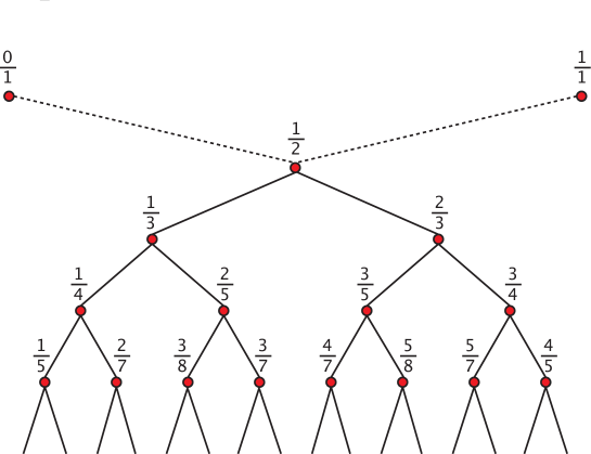
Figure 1: Farey tree.

A Farey sequence can be related to a graph construction known as Farey graph. A Farey graph ${\cal F}$ is a graph with vertex set on irreducible rational numbers between $0$ and $1$, and two rational numbers $p/q$ and $r/s$ are adjacent in ${\cal F}$ if and only if $rq-ps=1$ or $-1$, or equivalently if they are consecutive terms in some Farey sequence $F_{m}$. Note that the graph can be obtained from a subtree of the Farey tree by adding new edges, or equivalently, a subtree of the Farey tree is a spanning tree of a Farey graph. This graph was first introduced by Matula and Kornerup in 1979 and further studied by Colbourn in 1982, and has many interesting properties. For example, they are minimally 3-colorable, uniquely Hamiltonian, maximally outerplanar and perfect, see [18, 10, 7]

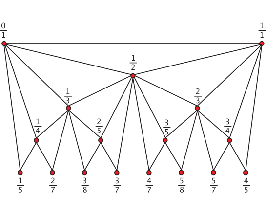
Figure 2: A Farey graph with 17 vertices.

In this paper we introduce a simple construction method for a family of Farey graphs, inspired by the mediant calculation of new nodes in the Farey tree. Other than the properties proved for general Farey graphs in [18, 10], we determine analytically, for this family of graphs, their order, size, degree distribution, degree correlations, clustering and transitivity coefficients, diameter, and average distance. The graphs are of interest as models for complex systems [22], as the parameters computed match those of their associated networks. They have small-world characteristics (a large clustering with small average distance) and they are minors of the pseudo-fractal networks [13] and Apollonian graphs [2], but in these cases the graphs are also scale-free (their degree distribution follows a power-law), see [4], while in our case the degrees follow an exponential distribution. However, relevant networks, which describe technological and biological systems, like some electronic circuits and protein networks are almost planar and have an exponential degree distribution [6, 14, 22]. This Farey graph family is also related to some random networks constructed following the method known as geographical attachment [25, 33].

2 Definition, order and size of the Farey graphs ${\cal F}(t)$

In this section we give an iterative construction method for a family of Farey graphs. When modeling real world networks with graphs, different methods have been considered: edge reconnection, duplication and addition of substructures, etc. Iterative methods that add new vertices at each step are useful as they can mimic processes that drive the network evolution through time. For example, in social, collaborative and some technological and biological networks it is very likely that a new node will join to nodes that are already adjacent. This suggests the following graph construction:

Definition 2.1

The graph ${\cal F}(t)=(V(t),E(t))$, $t\geq 0$, with vertex set $V(t)$ and edge set $E(t)$ is constructed as follows:

For $t=0$, ${\cal F}(0)$ has two vertices and an edge joining them.

For $t\geq 1$, ${\cal F}(t)$ is obtained from ${\cal F}(t-1)$ by adding to every edge introduced at step $t-1$ a new vertex adjacent to the endvertices of this edge.

.

Therefore, at $t=0$, ${\cal F}(0)$ is $K_{2}$, at $t=1$ the graph is $K_{3}$, at $t=2$ the graph has five vertices and seven edges, etc. Notice that the graph ${\cal F}(t)$, $t>1$, can also be constructed recursively from two copies of ${\cal F}(t-1)$, by identifying two initial vertices -one from each copy of ${\cal F}(t-1)$- and adding a new edge between the other two initial vertices, see Fig. 3.

In what follows we will call a generating edge an edge that, according to the definition 2.1, is used to introduce a new vertex in the next iteration step.

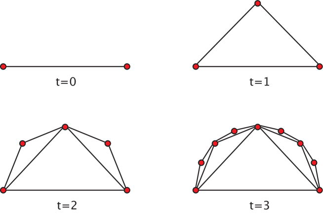
Figure 3: Farey graphs ${\cal F}(0)$ to ${\cal F}(3)$.

This graph construction is deterministic, and uses an iteration process similar to that of [13] where Dorogovtsev et al. introduced a graph, which they called “pseudofractal scale-free web” constructed as follows: At each step, for every edge of the graph (not only those introduced at the last step as in our graph construction), a new node is added, which is attached to the endvertices of the edge. In their construction the starting graph is $K_{3}$. This graph construction was generalized in [11]. All these graphs have relevant distinct properties with respect to the Farey graph family defined here. Finally, our graphs constitute the extreme case $q=0$ of the random construction in [33], where at each step an edge is chosen with probability $q$, and after the insertion of the new vertex and edges, the edge is removed.

We can see that our construction produces Farey graphs by labeling the vertices: if the two initial vertices are labeled $0/1$ and $1/1$, and each new added vertex is labeled with the mediant of the two vertices where it is joined, the vertices verify the definition of Farey graphs as given, for example, by Colbourn in [10] or Biggs in [7]. Therefore, as has been proved there, the graphs ${\cal F}(t)$ are minimally 3-colorable, uniquely Hamiltonian, maximally outerplanar and perfect.

Thanks to the deterministic nature of the graphs ${\cal F}(t)$, we can give exact values for the relevant topological properties of this graph family, namely, order, size, degree distribution, clustering, transitivity, diameter and average distance.

To find the order and size of ${\cal F}(t)$, we denote the number of new vertices and edges added at step $t$ by $L_{V}(t)$ and $L_{E}(t)$, respectively. These edges are generating edges.

Thus, initially ($t=0$), we have $L_{V}(0)=2$ vertices and $L_{E}(0)=1$ edges in ${\cal F}(0)$.

As each generating edge produces a new vertex and two generating edges at the next iteration, we have that $L_{V}(t)=L_{E}(t-1)$ and $L_{V}(t)=2\,L_{E}(t-1)$, which leads to $L_{E}(t)=2^{t}$ and $L_{V}(t)=2^{t-1}$

Therefore, the order of the graph is $|V(t)|=\sum_{i=0}^{t}L_{V}(i)$ and the total number of edges is $|E(t)|=\sum_{i=0}^{t}L_{E}(i)$ and we have:

Proposition 2.2

The order and size of the graph ${\cal F}(t)=(V(t),E(t))$ are, respectively,

$$|V(t)|=2^{t}+1\quad and\quad|E(t)|=2^{t+1}-1.$$ (1)

$\Box$

The average degree is $\bar{\delta(t)}=4-{3}/{(2^{t}+1)}$. For large $t$, it is small and approximately equal to $4$.

Many real-life networks are sparse in the sense that the number of links in the network is much less than $|V(t)|(|V(t)|-1)/2$, the maximum number of links [20, 1, 12, 22, 8].

3 Relevant characteristics of ${\cal F}(t)$

In this section we find analytically the degree distribution, degree correlations, clustering and transitivity coefficients, diameter and average distance of the graphs ${\cal F}(t)$.

3.1 Degree distribution

When studying networks associated with complex systems, the degree distribution is an important characteristic related to their topological, functional and dynamical properties. Most real life networks follow a power-law degree distribution and are called scale-free networks. However, relevant networks, which describe technological and biological systems, like some electronic circuits and protein networks have an exponential degree distribution [6, 14, 22]. The well known Watts-Strogatz small world network model also follows an exponential degree distribution [29] as it is the case of the Farey graphs analyzed here.

The degree distribution of ${\cal F}(t)$ is deduced from the following facts: Initially, at $t=0$, the graph has two vertices of degree one. When a new vertex $v$ is added to the graph at step $t_{c,v}$, this vertex has degree $2$ and it is connected to two generating edges. From the construction process, all vertices of the graph, except the initial two vertices, are always connected to two generating edges and will increase their degrees by two units at the next step.

Proposition 3.1

The cumulative degree distribution of the graph ${\cal F}(t)$ follows an exponential distribution ${\cal{P}}_{\mbox{\scriptsize cum}}(\delta)\sim 2^{-\frac{\delta}{2}}$

Proof.   We denote the degree of vertex $v$ at step $t$ by $\delta_{v}(t)$. By construction, we have

$$\delta_{v}(t+1) = \delta_{v}(t)+2\quad v\in V(t),v\neq{\small{0\over 1},{1\over 1}}$$

$$\delta_{0\over 1}(t) = \delta_{1\over 1}(t)=t+1$$ (2)

if $t_{c,v}$ ($t_{c,v}>0$) is the step at which a vertex $v$ is added to the graph, then $\delta_{v}(t_{c,v})=2$ and hence

$$\delta_{v}(t)=2(t-t_{c,v}+1).$$ (3)

Therefore, the degree distribution of the vertices of the graph ${\cal F}(t)$ is as follows: the number of vertices of degree $2\cdot 1,2\cdot 2,2\cdot 3,\cdots,2\cdot t$, equals, respectively, to $2^{t-1},2^{t-2},\ldots,2,1$ and the two initial vertices have degree $t+1$.

The degree distribution ${\cal{P}}(\delta)$ for a network gives the probability that a randomly selected vertex has exactly $\delta$ edges. In the analysis of the degree distribution of real life networks, see [17, 22], it is usual to consider their cumulative degree distribution,

$${\cal{P}}_{\mbox{\scriptsize cum}}(\delta)=\sum_{\delta^{\prime}=\delta}^{\infty}{\cal{P}}(\delta^{\prime}),$$

which is the probability that the degree of a vertex is greater than or equal to $\delta$.

Networks whose degree distributions are exponential: ${\cal{P}}(\delta)\sim e^{-\alpha\delta}$, have also an exponential cumulative distribution with the same exponent:

$${\cal{P}}_{\mbox{\scriptsize cum}}(\delta)=\sum_{\delta^{\prime}=\delta}^{\infty}P(\delta^{\prime})\approx\sum_{\delta^{\prime}=\delta}^{\infty}e^{-\alpha\delta^{\prime}}=\left(\frac{e^{\alpha}}{e^{\alpha}-1}\right)e^{-\alpha\delta}.$$ (4)

Because the contribution to the degree distribution of the two initial vertices of a Farey graph is small, we can use Eq. (3), and we have for ${\cal F}(t)$ that ${\cal{P}}_{\mbox{\scriptsize cum}}(\delta)\approx{\cal{P}}\left(t^{\prime}\leq\tau=t-\frac{\delta-2}{2}\right)$. Hence, for large $t$

$${\cal{P}}_{\mbox{\scriptsize cum}}(\delta)\approx\sum_{t^{\prime}=0}^{\tau}\frac{L_{V}(t^{\prime})}{|V(t)|}=\frac{2}{2^{t}+1}+\sum_{t^{\prime}=1}^{\tau}\frac{2^{t^{\prime}-1}}{2^{t}+1}=\frac{1+2^{\tau}}{1+2^{t}}\sim 2^{-\frac{\delta}{2}}.$$ (5)

$\Box$

3.2 Degree correlations

The study of degree correlations in a graph is a particularly interesting subject in the context of network analysis, as they account for some important network structure-related effects [19, 21, 22]. One first parameter is the average degree of the adjacent vertices for vertices with degree $\delta$ as a function of this degree value [26], which we denote as $k_{\rm nn}(\delta)$. When $k_{\rm nn}(\delta)$ increases with $\delta$, it means that vertices have a tendency to connect to vertices with a similar or larger degree. In this case the graph is called assortative [21]. In contrast, if $k_{\rm nn}(\delta)$ decreases with $\delta$, which implies that vertices of large degree are likely to be adjacent to vertices with small degree, then the graph is said to be disassortative. The graph is uncorrelated if $k_{\rm nn}(\delta)={\rm const}$.

We can obtain an exact analytical expression of $k_{\rm nn}(\delta)$ for the Farey graphs ${\cal F}(t)$. Note that except for the initial two vertices of step $0$, no vertices introduced at the same time step, which have the same degree, will be adjacent to each other. All adjacencies to vertices with a larger degree are produced when the vertex is added to the graph, and then the adjacencies to vertices with a smaller degree are made at each subsequent step. This results in the expression 3, i.e. $\delta=2(t-t_{c}+1)$, $t_{c}\geq 1$, and we can write:

$$k_{nn}(\delta)=\small\frac{1}{{L_{V}(t_{c})\delta(t_{c},t)}}\left[{2\!\!\sum\limits_{t^{\prime}_{c}=1}^{t_{c}-1}\!{L_{V}(t^{\prime}_{c},)\delta(t^{\prime}_{c},t)}+2\!\!\!\!\!\sum\limits_{t^{\prime}_{c}=t_{c}+1}^{t}\!\!\!\!\!{L_{V}(t_{c})\delta(t^{\prime}_{c},t)}+L_{V}(0)\delta(0,t)}\right]$$ (6)

where $\delta(t_{c},t)$ represents the degree of a vertex at step $t$, which was generated at step $t_{c}$. Here the first sum on the left-hand side accounts for the adjacencies made to vertices with larger degree (i.e. $0<t^{\prime}_{c}<t_{c}$) when the vertex was introduced at step $t_{c}$. The second sum represents the edges introduced to vertices with a smaller degree at each step $t^{\prime}_{c}>t_{c}$. And the last term explains the adjacencies made to the initial vertices of step $0$. Eq. (6) leads to

$$k_{nn}(\delta)=t-t_{c}+2+\frac{4}{{t-t_{c}+1}}-\frac{{(t+3)\cdot 2^{1-t_{c}}}}{{t-t_{c}+1}}.$$ (7)

Writing Eq. (7) in terms of $\delta$, we have

$$k_{nn}(\delta)=\frac{\delta}{2}+\frac{8}{\delta}+1-\frac{(t+3)\cdot 2^{1+\delta/2}}{\delta\cdot 2^{t}}.$$ (8)

Thus we have obtained the degree correlations for those vertices generated at step $t_{c}\geq 1$. For the initial two vertices, as each has degree $\delta_{0}=t+1$, we obtain

$$k_{nn}(\delta_{0})=\frac{1}{\delta_{0}}\sum\limits_{t^{\prime}_{c}=0}^{t}{\delta(t^{\prime}_{c},t)=}\delta_{0}.$$ (9)

From Eqs. (8) and (9), it is obvious that for large graphs (i.e. $t\rightarrow\infty$), $k_{nn}(\delta)$ is approximately a linear function of $\delta$, which suggests that Farey graphs are assortative.

Degree correlations can also be described by the Pearson correlation coefficient $r$ of the degrees of the endvertices of the edges. For a general graph $G(V,E)$, this coefficient is defined as [21]

$$r=\frac{|E(t)|\sum_{i}j_{i}k_{i}-[\sum_{i}\frac{1}{2}(j_{i}+k_{i})]^{2}}{|E(t)|\sum_{i}\frac{1}{2}(j_{i}^{2}+k_{i}^{2})-[\sum_{i}\frac{1}{2}(j_{i}+k_{i})]^{2}}$$ (10)

where $j_{i}$, $k_{i}$ are the degrees of the endvertices of the $i$th edge, with $i=1,\cdots,|E(t)|$. This coefficient is in the range $-1\leq r\leq 1$. If the graph is uncorrelated, the correlation coefficient equals zero. Disassortative graphs have $r<0$, while assortative graphs have a value of $r>0$.

If $r(t)$ denotes the Pearson degree correlation of ${\cal F}(t)$, we have

Proposition 3.2

The Pearson degree correlation coefficient of the graph ${\cal F}(t)$ is

$$r(t)=\frac{16\cdot 2^{2t}-2^{t}(4t^{3}+6t^{2}-40t-26)-(t^{4}+10t^{3}+43t^{2}+80t+2)}{64\cdot 2^{2t}-2^{t}(6t^{3}+18t^{2}-6t+46)-(t^{4}+9t^{3}+37t^{2}+63t+18)}$$

Proof.   We find the degrees of the endvertices for every edge of the Farey graph. Let $\langle j_{i},k_{i}\rangle$ stand for the $i$th edge in ${\cal F}(t)$ connecting two vertices with degrees $j_{i}$ and $k_{i}$. Then the initial edge created at step $0$ can be expressed as $\langle t+1,t+1\rangle$. By construction, at step $t_{c}$ ($t_{c}\geq 1$), $2^{t_{c}}$ new edges are added to the graphs. Each new iteration will increase the degree of these vertices. These edges connect new vertices, which have degree 2, to every vertex in ${\cal F}(t_{c}-1)$ which have the following degree distribution at step $t_{c}-1$: $\delta(l,t_{c}-1)=2(t_{c}-l)$ ($1\leq l\leq t_{c}-1$) and $\delta(0,t_{c}-1)=t_{c}$. At each of the subsequent steps of $t_{c}-1$, all these vertices will increase their degrees by two, except the two initial vertices, the degree of which grow by one unit. Thus, at step $t$, the number of edges $\langle 2(t-t_{c}+1),2(t-l+1)\rangle$ ($1\leq l\leq t_{c}-1$) is $2^{l}$ and the number of edges $\langle 2(t-t_{c}+1),t+1\rangle$ is 2.

Now we can explicitly find the sums in Eq. 10:

$$\sum\limits_{m=1}^{|E(t)|}j_{m}k_{m} = -79+5\cdot 2^{4+t}-52t-15t^{2}-2t^{3},$$

$$\sum\limits_{m=1}^{|E(t)|}(j_{m}+k_{m}) = -22+3\cdot 2^{3+t}-12t-2t^{2},$$

$$\sum\limits_{m=1}^{|E(t)|}(j_{m}^{2}+k_{m}^{2}) = -206+13\cdot 2^{4+t}-138t-42t^{2}-6t^{3},$$

which lead to the stated result.  $\Box$

We can easily see that for $t$ large, $r(t)$ tends to the value $\frac{1}{4}$, which again indicates that the Farey graphs are assortative.

3.3 Clustering coefficient

The clustering coefficient of a graph is another parameter used to characterize small-world networks. The clustering coefficient of a vertex was introduced in [29] to quantify this concept: Given a graph $G=(V,E)$, for each vertex $v\in V(G)$ with degree $\delta_{v}$, its clustering coefficient $c(v)$ is defined as the fraction of the ${\delta_{v}\choose 2}$ possible edges among the neighbors of $v$ that are present in $G$. More precisely, if $\epsilon_{v}$ is the number of edges between the $\delta_{v}$ vertices adjacent to vertex $v$, its clustering coefficient is

$$c(v)=\frac{2\epsilon_{v}}{\delta_{v}(\delta_{v}-1)},$$ (11)

whereas the clustering coefficient of $G$, denoted by $c(G)$, is the average of $c(v)$ over all vertices $v$ of $G$:

$$c(G)=\frac{1}{|V(G)|}\sum_{v\in V(G)}c(v).$$ (12)

Some authors, see for example [24], use another definition of clustering coefficient of $G$:

$$c^{\prime}(G)=\frac{3\,T(G)}{\tau(G)}$$ (13)

where $T(G)$ and $\tau(G)$ are, respectively, the number of triangles (subgraphs isomorphic to $K_{3}$) and the number of triples (subgraphs isomorphic to a path on $3$ vertices) of $G$. A triple at a vertex $v$ is a $3$-path with central vertex $v$. Thus the number of triples at $v$ is

$$\tau(v)={\delta_{v}\choose 2}=\frac{\delta_{v}(\delta_{v}-1)}{2}.$$ (14)

The total number of triples of $G$ is denoted by $\tau(G)=\sum_{v\in V(G)}\tau(v)$.

Using these parameters, note that the clustering coefficient of a vertex $v$ can also be written as $c(v)=\frac{T(v)}{\tau(v)}$, where $T(v)={\delta_{v}\choose 2}$ is the number of triangles of $G$ which contain vertex $v$. From this result, we see that $c(G)=c^{\prime}(G)$ if, and only if,

$$|V(G)|=\frac{\sum_{v\in V(G)}\tau(v)}{\sum_{v\in V(G)}T(v)}\sum_{v\in V(G)}\frac{T(v)}{\tau(v)}.$$

And this is true for regular graphs or for graphs such that all vertices have the same clustering coefficient. $c^{\prime}(G)$ is known in the context of social networks as transitivity coefficient.

We compute here both the clustering coefficient and the transitivity coefficient.

Proposition 3.3

The clustering coefficient $c({\cal F}(t))$ of the graph ${\cal F}(t)$ is

$$c({\cal F}(t))=\frac{1}{2^{t}+1}\left[2^{t}\ln 2-\frac{1}{2}\Phi\left(\frac{1}{2},1,1+t\right)+\frac{4}{t+1}\right]$$ (15)

where $\Phi$ denotes the Lerch’s transcendent function.

Proof.   When a new vertex $v$ joins the graph, its degree is $\delta_{v}=2$ and $\epsilon_{v}$ equals 1. Each subsequent addition of an edge to this vertex increases both parameters by one. Thus, $\epsilon_{v}$ equals to $\delta_{v}-1$ for all vertices at all steps. Therefore there is a one-to-one correspondence between the degree of a vertex and its clustering. For a vertex $v$ of degree $\delta_{v}$, the expression for its clustering coefficient is $c(v)=2/\delta_{v}$. It is interesting to note that this scaling of the clustering coefficient with the degree has been observed empirically in several real-life networks [27]. The same value has also been obtained in other models [25, 32, 31, 13].

We use the degree distribution found above to calculate the the clustering coefficient of the graph ${\cal F}(t)$. Clearly, the number of vertices with clustering coefficient $1$, $\frac{1}{2}$, $\frac{1}{3}$, $\cdots$, $\frac{1}{t-1}$, $\frac{1}{t}$, $\frac{2}{t+1}$ , is equal to $2^{t-1},2^{t-2},\ldots,2,1,2$, respectively.

Thus, the clustering coefficient of the graph $c({\cal F}(t))$ is easily obtained for any arbitrary step $t$:

$$c({\cal F}(t)) = \frac{1}{|V(t)|}\left[\sum_{i=1}^{t}\frac{1}{i}\cdot 2^{t-i}+\frac{2}{t+1}\cdot 2\right]$$ (16)

$$= \frac{1}{2^{t}+1}\left[2^{t}\ln 2-\frac{1}{2}\Phi\left(\frac{1}{2},1,1+t\right)+\frac{4}{t+1}\right].$$

$\Box$

The clustering coefficient $c({\cal F}(t))$ tends to $\ln 2$ for large $t$. Thus the clustering coefficient of ${\cal F}(t)$ is high.

To find the transitivity coefficient we need to calculate the number of triangles and the number of triples of the graph.

Lemma 3.4

The number of triangles of ${\cal F}(t)$ is

$$T({\cal F}(t))=2^{t}-1,t\geq 1$$

Proof.   At a given step $t$ the number of new triangles introduced to the graph is the number of generating edges, which are the edges introduced in the former step $L_{E}(t)=2^{t-1}$. Therefore $T({\cal F}(t))=T({\cal F}(t-1))+2^{t-1}$, and as $T({\cal F}(1))=1$, we have the result.  $\Box$

Moreover, again from the results found above giving the number of vertices of each degree, we obtain straightforwardly the following result for the number of triples:

Lemma 3.5

The number of triples of ${\cal F}(t)$ is

$$\tau({\cal F}(t))=5\cdot 2^{t+1}-t^{2}-6\cdot t-10$$

$\Box$

Now the transitivity coefficient follows from the former two lemmas.

Proposition 3.6

The transitivity coefficient of ${\cal F}(t)$ is:

$$c^{\prime}({\cal F}(t))=\frac{3\cdot 2^{t}-3}{10\cdot 2^{t}-t^{2}-6t-10}$$

We see that while the clustering coefficient increases with $t$ and tends to $\ln 2$, the transitivity coefficient tends to $0.3$.

The small-world concept describes the fact that, in many real-life networks, there is a relatively short distance between any pair of nodes. In this case we will expect an average distance, and in some cases a diameter, which scales logarithmically with the graph order. Next we verify this two relations for the Farey graphs ${\cal F}(t)$.

3.4 Diameter

Computing the exact diameter of ${\cal F}(t)$ can be done analytically, and gives the result shown below.

Proposition 3.7

The diameter of the graph ${\cal F}(t)$ is $diam({\cal F}(t))=t$, $t\geq 1$.

Proof.   Clearly, at steps $t=0$ and $t=1$, the diameter is 1.

At each step $t\geq 2$, by the construction process, the longest path between a pair of vertices is for some vertices added at this step. Vertices added at a given step $t\geq 1$ are not adjacent among them and are always connected to two vertices that were introduced at different former steps. Now consider two vertices introduced at step $t\geq 2$, say $v_{t}$ and $w_{t}$. $v_{t}$ is adjacent to two vertices, and one of them must have been added to the graph at step $t-2$ or a previous one. We consider two cases: (a) For $t=2m$ even and from $v_{t}$ we reach in $m$ “jumps” a vertex of the graph ${\cal F}(0)$, which we can also reach from $w_{t}$ in a similar way. Thus $diam({\cal F}(2m))\leq 2m$. (b) $t=2m+1$ is odd. In this case we can stop after $m$ jumps at ${\cal F}(1)$, for which we know that the diameter is 1, and make $m$ jumps in a similar way to reach $w_{t}$. Thus $diam({\cal F}(2m+1))\leq 2m+1$. This bound is reached by pairs of vertices created at step $t$. More precisely, by those two vertices $v_{t}$ and $w_{t}$ which have the property of being connected to two vertices introduced at steps $t-1$, $t-2$. Hence, $diam({\cal F}(t))=t$ for any $t\geq 1$.  $\Box$

As $\log|V({\cal F}(t))|=t\cdot\ln 2$, for large $t$ we have $diam({\cal F}(t))\sim\ln|V({\cal F}(t))|$.

Because the graph ${\cal F}(t)$ is sparse, has a high clustering and a small, logarithmic, diameter (and also a logarithmic average distance, as we will prove next) our model shows small-world characteristics [29].

Next we find the exact analytical expression for the average distance of the graphs ${\cal F}(t)$.

3.5 Average distance

Given a graph $G=(V,E)$ its average distance or mean distance is defined as: $\mu(G)=\frac{1}{|V(G)|(|V(G)|-1)}\sum_{u,v\in V(G)}d(u,v)$ where $d(u,v)$ is the distance between vertices $u$ and $v$ of $V(G)$.

The recursive construction of ${\cal F}(t)$ allows to obtain the exact value of $\mu({\cal F}(t))$:

Proposition 3.8

The average distance of ${\cal F}(t)$ is

$$\mu({\cal F}(t))=\frac{2^{2t}(6t-5)+2^{t}(6t+17)+5+(-1)^{t}}{9\cdot 2^{2t}+9\cdot 2^{t}}.$$

Proof.   First we find a recurrence formula to obtain transmission coefficient $\sigma({\cal F}(t+1))$ from $\sigma({\cal F}(t))$ using the recursive construction of ${\cal F}(t)$ As shown in Fig. 4, the graph ${\cal F}(t+1)$ may be obtained by joining at three boundary vertices ($X$, $Y$, and $Z$) two copies of ${\cal F}(t)$ that we will label as $F_{t}^{(\eta)}$ with $\eta=1,2$. According to this construction method, the transmission $\sigma({\cal F}(t))$ satisfies the recursive relation

$$\sigma({\cal F}(t+1)))=2\sigma({\cal F}(t))+S_{t},$$ (17)

where $S_{t}$ denotes the sum of distances of pairs of vertices which are not both in the same $F_{t}^{(\eta)}$ subgraph.

Figure 4: Schematic illustration of the recursive construction of the Farey graph. ${\cal F}(t+1)$ may be obtained by joining two copies of ${\cal F}(t)$, denoted as $F_{t}^{(1)}$ and $F_{t}^{(2)}$, which are connected to each other as shown.

To calculate $S_{t}$, we classify the vertices in ${\cal F}(t+1)$ into two categories: vertices $X$ and $Y$ (see figure 4) are called connecting vertices, while the other vertices are called interior vertices. Thus $S_{t}$ is obtained by considering the following distances: between interior vertices in one $F_{t}^{(\eta)}$ subgraph to interior vertices in the other $F_{t}^{(\eta)}$ subgraph, between a connecting vertex from one $F_{t}^{(\eta)}$ subgraph and all the interior vertices in the other $F_{t}^{(\eta)}$ subgraph, and between the two connecting vertices $X$ and $Y$ (i.e. $d(XY)=1$).

Let us denote by $S_{t}^{1,2}$ the sum of all distances between the interior vertices, of $F_{t}^{(1)}$ and $F_{t}^{(2)}$. Notice that $S_{t}^{1,2}$ does not count paths with endpoints at the connecting vertices $X$ and $Y$. On the other hand, let $\Omega_{t}^{(\eta)}$ be the set of interior vertices in $F_{t}^{(\eta)}$. Then the total sum $S_{t}$, using the symmetry $\sum_{j\in\Omega_{t}^{2}}d(X,j)=\sum_{j\in\Omega_{t}^{1}}d(Y,j)$, is given by

$$S_{t}=S_{t}^{1,2}+\sum_{j\in\Omega_{t}^{(2)}}d(X,j)+\sum_{j\in\Omega_{t}^{(1)}}d(Y,j)+d(X,Y)=S_{t}^{1,2}+2\,\sum_{j\in\Omega_{t}^{(2)}}d(X,j)+1.$$ (18)

We obtain $S_{t}^{1,2}$ by classifying all interior vertices of ${\cal F}(t+1)$ into three different sets according to their distances to the two connecting vertices $X$ or $Y$. Notice that these two vertices themselves are not included into any of the three sets which are denoted $P_{1}$, $P_{2}$, and $P_{3}$, respectively. This classification is shown schematically in Fig. 5. By construction, $d(v,X)$ and $d(v,Y)$ can differ by at most $1$ since vertices $X$ and $Y$ are adjacent. Then the classification function $class(v)$ of a vertex $v$ is defined as

$$class(v)=\left\{\begin{array}[]{lc}{\displaystyle{P_{1}}}&\quad\hbox{if}\ d(v,X)<d(v,Y),\\ {\displaystyle{P_{2}}}&\quad\hbox{if}\ d(v,X)=d(v,Y),\\ {\displaystyle{P_{3}}}&\quad\hbox{if}\ d(v,X)>d(v,Y).\\ \end{array}\right.$$ (19)

Figure 5: Illustration of the vertex classification of $F_{t}^{(1)}$ and $F_{t}^{(2)}$, used to find recursively the classification of all the interior vertices of the graph. ${\cal F}(t+1)$.

This definition of vertex classification is recursive. For instance, classes $P_{1}$ and $P_{2}$ of $F_{t}^{(1)}$ are in class $P_{1}$ of $F_{t+1}^{(1)}$ and class $P_{3}$ of $F_{t}^{(1)}$ is in class $P_{2}$ of $F_{t+1}^{(1)}$. Since the two vertices $X$ and $Y$ play a symmetrical role, classes $P_{1}$ and $P_{3}$ are equivalent. We denote the number of vertices in $F_{t}$ that belong to class $P_{i}$ ($i=1,2,3$) as $N_{t,P_{i}}$. By symmetry, $N_{t,P_{1}}=N_{t,P_{3}}$. Therefore we have:

$$|V(t)|=N_{t,P_{1}}+N_{t,P_{2}}+N_{t,P_{3}}+2=2\,N_{t,P_{1}}+N_{t,P_{2}}+2.$$

Considering the self-similar structure of the Farey graph, we can write the following recursive expression for $N_{t+1,P_{1}}$ and $N_{t+1,P_{2}}$:

$$\begin{array}[]{ccc}N_{t+1,P_{1}}&=&\,N_{t,P_{1}}+\,N_{t,P_{2}}\,,\\ N_{t+1,P_{2}}&=&2\,N_{t,P_{1}}+1\,,\\ \end{array}$$

Together with the initial conditions $N_{1,P_{1}}=N_{1,P_{2}}=0$ we find:

$$\begin{array}[]{ccc}N_{t,P_{1}}&=&\frac{1}{6}\left(2^{t+1}-3+(-1)^{t}\right),\\ N_{t,P_{2}}&=&\frac{1}{3}\left(2^{t}-(-1)^{t}\right).\\ \end{array}$$ (23)

For a vertex $v$ of ${\cal F}(t+1)$, we are also interested in the distance from $v$ to either of the two border connecting vertices $X$ and $Y$ and we denote it by $\ell_{v}=min(d(v,X),d(v,Y))$.

Let $\ell_{t,P_{i}}(i=1,2,3)$ denote the sum of $\ell_{v}$ for all the vertices which are in class $P_{i}$ of $F_{t}^{(\eta)}$. Again by symmetry, we have $\ell_{t,P_{1}}=\ell_{t,P_{3}}$, and thus $\ell_{t,P_{1}}$, $\ell_{t,P_{2}}$ can be written recursively as follows:

$$\begin{array}[]{ccc}\ell_{t+1,P_{1}}&=&\,\ell_{t,P_{1}}+\ell_{t,P_{2}}\,,\\ \ell_{t+1,P_{2}}&=&2\,\ell_{t,P_{1}}+N_{t,P_{1}}+1\,.\\ \end{array}$$ (26)

Substituting Eq. (23) into Eq. (26), and considering the initial conditions $\ell_{1,P_{1}}=0$ and $\ell_{1,P_{2}}=0$, Eq. (26) can be solved and we obtain:

$$\begin{array}[]{ccc}\ell_{t,P_{1}}&=&\frac{1}{81}\Big{(}9\cdot t\cdot(-1)^{t}+9\cdot t\cdot 2^{t}-(-1)^{-t}+2^{-t}+4(-1)^{t}-\\ &&\qquad-3\cdot 2^{t}-(-2)^{-t}(-1)^{3t}\Big{)},\hfill\\ \ell_{t,P_{2}}&=&\frac{1}{81}(-2)^{-t}\Big{(}9(-4)^{t}t+15(-4)^{t}-2(-1)^{t}+2(-1)^{3t}-\\ &&\qquad-2^{t}\left(2(-1)^{2t}(9t+7)+1\right)\Big{)}.\hfill\end{array}$$ (31)

After obtaining the values $N_{t,P_{i}}$ and $\ell_{t,P_{i}}$ ($i=1,2,3$), we next will find $S_{t}^{1,2}$ and $\sum_{j\in\Omega_{t}^{(2)}}d(X,j)$ expressed as a function of $N_{t,P_{i}}$ and $\ell_{t,P_{i}}$. For convenience, we use $\Omega_{t}^{(\eta),i}$ to denote the set of interior nodes belonging to class $P_{i}$ in $F_{t}^{(\eta)}$. Then $S_{t}^{1,2}$ can be written as

$$S_{t}^{1,2} = \sum_{\begin{subarray}{c}u\in\Omega_{t}^{(1),1},\,\,v\in F_{t}^{(2)}\\ v\neq Y,Z\end{subarray}}\!\!\!\!\!\!\!\!\!\!d(u,v)+\sum_{\begin{subarray}{c}u\in\Omega_{t}^{(1),2},\,\,v\in F_{t}^{(2)}\\ v\neq Y,Z\end{subarray}}\!\!\!\!\!\!\!\!\!\!d(u,v)+\sum_{\begin{subarray}{c}u\in\Omega_{t}^{(1),3},\,\,v\in F_{t}^{(2)}\\ v\neq Y,Z\end{subarray}}\!\!\!\!\!\!\!\!\!\!d(u,v)\,.$$ (32)

Next we calculate the first term on the right side of Eq. (32).

$$\sum_{\begin{subarray}{c}u\in\Omega_{t}^{(1),1},\,\,v\in F_{t}^{(2)}\\ v\neq Y,Z\end{subarray}}\!\!\!\!\!\!\!\!\!\!d(u,v)=\sum_{u\in\Omega_{t}^{(1),1},\,v\in\Omega_{t}^{(2),1}\bigcup\Omega_{t}^{(2),2}}\!\!\!\!\!\!\!\!\!\!(d(u,X)+d(X,Z)+d(Z,v))$$

$$+\sum_{u\in\Omega_{t}^{(1),1},\,v\in\Omega_{t}^{(2),3}}\!\!\!\!\!\!\!\!\!\!(d(u,X)+d(X,Y)+d(Y,v))=$$

$$= N_{t,P_{1}}(2\ell_{t,P_{1}}+\ell_{t,P_{2}}+2N_{t,P_{1}}+N_{t,P_{2}})+\ell_{t,P_{1}}(2\,N_{t,P_{1}}+N_{t,P_{2}}).$$

Proceeding similarly, we obtain for the second term

$$N_{t,P_{2}}(2\ell_{t,P_{1}}+\ell_{t,P_{2}}+N_{t,P_{1}})+\ell_{t,P_{2}}(2\,N_{t,P_{1}}+N_{t,P_{2}}),$$

and finally, for the third term

$$N_{t,P_{1}}(2\ell_{t,P_{1}}+\ell_{t,P_{2}}+N_{t,P_{1}})+\ell_{t,P_{1}}(2\,N_{t,P_{1}}+N_{t,P_{2}}).$$

This leads to

$$S_{t}^{1,2}=2(2\ell_{t,P_{1}}+\ell_{t,P_{2}})(2\,N_{t,P_{1}}+N_{t,P_{2}})+N_{t,P_{1}}(3N_{t,P_{1}}+2N_{t,P_{2}}).$$ (33)

Analogously, we find

$$\sum_{j\in\Omega_{t}^{2}}d(X,j)=(2\ell_{t,P_{1}}+\ell_{t,P_{2}})+(2\,N_{t,P_{1}}+N_{t,P_{2}}).$$ (34)

Substituting Eqs. (33) and (34) into Eq. (18) and using Eq. (31) we have the final expression for $S_{t}$,

$$S_{t}=\frac{1}{18}\left[-5-3(-1)^{t}+12\cdot 2^{t}+14\cdot 2^{2t}+12\,t\cdot\,4^{t}\right].$$ (35)

With these results and recursion relations, we finally find the transmission coefficient. Inserting Eq. (35) into Eq. (17) and using the initial condition $\sigma({\cal F}(0))=1$, Eq. (17) can be solved inductively,

$$\sigma({\cal F}(t))=\frac{1}{18}\left[5+(-1)^{t}+(6t+17)2^{t}+(6t-5)4^{t}\right]$$ (36)

which together with the graph order leads to the stated result:

$$\mu({\cal F}(t))=\frac{2^{2t}(6t-5)+2^{t}(6t+17)+5+(-1)^{t}}{9\cdot 2^{2t}+9\cdot 2^{t}}.$$

$\Box$

Notice that for a large iteration step $t$ $\mu({\cal F}(t))\sim t\sim\ln|V_{t}|$, which shows a logarithmic scaling of the average distance with the order of the graph. This logarithmic scaling of $\mu({\cal F}(t))$ with the graph order, together with the large clustering coefficient $c({\cal F}(t))=\ln 2$ obtained in the preceding section, shows that the Farey graph has small-world characteristics.

4 Conclusion

We have introduced and studied a family of Farey graphs, based on Farey sequences, which are minimally 3-colorable, uniquely Hamiltonian, maximally outerplanar, perfect, modular, have an exponential degree hierarchy, and are also small-world. A combination of modularity, exponential degree distribution, and small-world properties can be found in real networks like some social and technical networks, in particular some electronic circuits, and those related to several biological systems (metabolic networks, protein interactome, etc) [22, 14].

On the other hand, the graphs are outerplanar and many algorithms that are NP-complete for general graphs run in polynomial time in outerplanar graphs [9]. This should help to find efficient algorithms for graph and network dynamical processes (communication, hub location, routing, synchronization, etc).

Finally, another interesting property of this graph family is its deterministic character which should facilitate the exact calculation of some other graph parameters and invariants and the development of algorithms.

References

- [1] R. Albert and A.-L. Barabási, Statistical mechanics of complex networks, Rev. Mod. Phys. 74 (2002) 47.
- [2] J. S. Andrade Jr., H. J. Herrmann, R. F. S. Andrade and L. R. da Silva, Apollonian Networks: Simultaneously scale-free, small world, Euclidean, space filling, and with matching graphs. Phys. Rev. Lett. 94(2005) 018702.
-
[3]
D. Austin,
Trees, Teeth, and Time: The mathematics of clock making,
American Mathematical Society. Feature Column. Monthly Essays on Mathematical Topics. December 2008.
http://www.ams.org/featurecolumn/archive/stern-brocot.html - [4] A.-L. Barabási, R. Albert, Emergence of scaling in random networks, Science 286 (1999) 509–512.
- [5] M. Barthélémy and L. A. N. Amaral, Small-World Networks: Evidence for a Crossover Picture, Phys. Rev. Lett. 82 (1999) 3180.
- [6] A. Barrat, M. Weigt, On the properties of small-world network models, Eur. Phys. J. B 13 (2000) 547–560.
- [7] N. L. Biggs, Graphs with large girth, Ars Combinatoria 25-C (1988) 73–80.
- [8] S. Boccaletti, V. Latora, Y. Moreno, M. Chavez, D.-U. Hwang, Complex networks: Structure and dynamics, Phy. Rep. 424 , 175 (2006).
- [9] A. Brandstaedt, V. B. Le, P. J. Spinrad, Graph Classes: A Survey, SIAM Monographs on Discrete Mathematics and Applications. Philadelphia, PA, 1999.
- [10] C. J. Colbourn, Farey series and maximal outerplanar graphs, Siam J. Alg. Disc. Meth. 3 (1982) 187–189.
- [11] F. Comellas, G. Fertin, and A. Raspaud , Recursive graphs with small-world scale-free properties, Phys. Rev. E 69 (2004) 037104
- [12] S. N. Dorogovtsev and J.F.F. Mendes, Evolution of networks, Adv. Phys. 51 (2002) 1079 .
- [13] S. N. Dorogovtsev, A. V. Goltsev, and J. F. F. Mendes, Pseudofractal scale-free web, Phys. Rev. E 65 (2002), 066122.
- [14] R. Ferrer i Cancho, C. Janssen, R. V. Solé, Topology of technology graphs: Small world patterns in electronic circuits, Phys. Rev. E 64 (2001) 046119
- [15] R. L. Graham, D. E. Knuth, and O. Patashnik. Concrete Mathematics: A Foundation for Computer Science, Addison-Wesley Pub. Co., Reading Ma. 1985.
- [16] G. H. Hardy and E. M. Wright. An Introduction to the Theory of Numbers. Oxford University Press. 5th edition. (1979)
- [17] S. Jung, S. Kim, and B. Kahng, Geometric fractal growth model for scale-free networks, Phys. Rev. E 65 (2002) 056101.
- [18] D. W. Matula and P. Kornerup. A graph theoretic interpretation of fractions, continued fractions and the GCD algorithm. Proc. 10th Southeastern Conference on Combinatorics, Graph Theory, and Computing. R.C. Mullin, and R.G. Stanton (eds), Utilitas Mathematica Publishing, Inc., 1979, pp. 932.
- [19] S. Maslov and K. Sneppen, Specificity and stability in topology of protein networks, Science 296 (2002) 910–913.
- [20] M. E. J. Newman,, Models of small-world, J. Stat. Phys. 101 (2000) 819.
- [21] M. E. J. Newman, Assortative mixing in networks, Phys. Rev. Lett. 89 (2002) 208701.
- [22] M. E. J. Newman, The structure and function of complex networks, SIAM Rev. 45 (2003) 167–256.
- [23] M. E. J. Newman and D.J. Watts, Renormalization group analysis of the small-world network model, Phys. Lett. A 263, 341 (1999).
- [24] M. E. J. Newman, D. J. Watts, and S. H. Strogatz, Random graph models of social networks, Proc. Natl. Acad. Sci. U.S.A. 99 (2002) 2566–2572.
- [25] J. Ozik, B.-R. Hunt, and E. Ott, Growing networks with geographical attachment preference: Emergence of small worlds, Phys. Rev. E 69 (2004) 026108.
- [26] R. Pastor-Satorras, A. Vázquez, and A. Vespignani, Dynamical and correlation properties of the Internet, Phys. Rev. Lett. 87 (2001) 258701.
- [27] E. Ravasz and A.-L. Barabási, Hierarchical organization in complex networks, Phys. Rev. E 67 (2003), 026112.
- [28] R. V. Solé and S. Valverde, Information theory of complex networks: on evolution and architectural constraints, Lecture Notes in Phys. 650 (2004) 189–207.
- [29] D. J. Watts and S.H. Strogatz, Collective dynamics of ‘small-world’ networks, Nature 393 (1998) 440–442.
-
[30]
E.W. Weisstein,
”Farey Sequence.” From MathWorld–A Wolfram Web
Resource.
http://mathworld.wolfram.com/FareySequence.html - [31] Z. Zhang, L. Rong, and F. Comellas, Evolving small-world networks with geographical attachment preference, J. Phys. A: Math. Gen. 39 (2006) 3253–3261.
- [32] Z. Z. Zhang, L. L. Rong, and C. H. Guo, A deterministic small-world network created by edge iterations, Physica A 363 (2006), 567-572.
- [33] Z. Zhang, S. Zhou, Z. Wang, and Z. Shen, A geometric growth model interpolating between regular and small-world networks, J. Phys. A: Math. Theor. 40 (2007) 11863-11876.