Pseudospin in optical and transport properties of graphene

Abstract

We show that the pseudospin being an additional degree of freedom for carriers in graphene can be efficiently controlled by means of the electron-electron interactions which, in turn, can be manipulated by changing the substrate. In particular, an out-of-plane pseudospin component can occur leading to a zero-field Hall current as well as to polarization-sensitive interband optical absorption.

Introduction. The charge carriers in graphene are described at low energies by an effective Hamiltonian being formally equivalent to the massless two-dimensional Dirac HamiltonianNovoselov et al. (2005); Geim and Novoselov (2007); Castro Neto et al. (2009), $H^{\nu}_{0}=\hbar v_{0}(\nu\sigma_{x}k_{x}+\sigma_{y}k_{y})$, where $\nu=\pm$ refers to the two inequivalent corners $K$, $K^{\prime}$ of the first Brillouin zone, $v_{0}\approx 10^{6}\mathrm{ms^{-1}}$ is the effective “speed of light”, ${\mathbf{k}}$ is the two-component particle momentum operator, and $\sigma_{x,y}$ are Pauli matrices describing the sublattice degree of freedom also referred to as the pseudospinCastro Neto et al. (2009). In the original Dirac Hamiltonian the Pauli vector $\vec{\sigma}$ represents the spin of a spin-$1/2$ particle which can be detected in Stern–Gerlach-like experiments. The pseudospin in graphene is formally similar to the true electron spin with an important distinction given by the behavior under time and parity Kane and Mele (2005) inversion. For the above effective model the time reversal operator $T$ is just the operator $C$ of complex conjugation, $T=C$, fulfilling $TH^{\nu}_{0}T^{-1}=H^{-\nu}_{0}$, and the operators $H^{+}_{0}$ and $H^{-}_{0}$ get interchanged. On the other hand, if one would (formally!) interpret the Pauli matrices as components of a genuine spinMecklenburg and Regan (2011) (i.e. an angular momentum), the time reversal operator would read $\tilde{T}=\sigma_{y}C$ giving $\tilde{T}H^{\nu}_{0}\tilde{T}^{-1}=H^{\nu}_{0}$. The parity operator $P$ flips the sign of the spatial coordinates interchanging the two sublattices and, similar to $T$, fulfills $PH_{0}^{\nu}P^{-1}=H_{0}^{-\nu}$. Thus, the initial Hamiltonian $H^{+}_{0}+H^{-}_{0}$ is $PT$-invariant but, as we shall see, the exchange interactions can break either invariance. It also is important that the pseudospin is not linked with the internal magnetic moment of an electron and does not directly interact with the external magnetic field prohibiting Stern–Gerlach type experiments. In contrast to that, we predict situations where the pseudospin manifests itself in observable quantities and can be detected in transport as well as optical measurements on graphene.

First of all we show that the exchange electron-electron interaction can alter the pseudospin orientation in a very broad range. In an eigenstate of $H^{\nu}_{0}$ the pseudospin is always in the $xy$-plane. As we shall see shortly, the exchange interactions can turn the pseudospin texture to the out-of-plane phase with the out-of-plane angle depending on the absolute value of the particle momentum. This is due to the huge negative contribution to the Hartree–Fock ground state energy from the valence band (i. e. “antiparticle” states) which cannot be neglected in graphene because of the zero gap (i. e. zero effective mass of carriers) and large effective fine structure constant $\alpha^{*}=e^{2}/(\varepsilon\hbar v_{0})$ where $\varepsilon$ is the dielectric constant depending on the environmentJang et al. (2008). The exchange contribution to the ground state energy has previously been studied in both monolayer and bilayer graphene regarding properties such as the electronic compressibilityMartin et al. (2008) and ferromagnetismPeres et al. (2005); Barlas et al. (2007); Nilsson et al. (2006), but the importance of the interplay between pseudospin and electron-electron interactions has been recognized only in Min et al. (2008) where single layer graphene was mentioned in passing.

Having established the possibility to create an out-of-plane pseudospin orientation by means of the exchange interaction, we apply the Boltzmann approach to derive the electrical conductivity tensor which turns out to have Hall components even though the external magnetic field is absent. The mechanism of this phenomenon is intimately linked to the pseudospin-momentum coupling which can be read out immediately from the Hamiltonian $H^{\nu}_{0}$. Similar to the skew scattering of electrons on impurities in spin-orbit coupled systems partly responsible for the anomalous Hall effectNagaosa et al. (2010); Sinitsyn (2008), the carriers in graphene do also skew to one side of the Hall bar as long as their pseudospin has non-zero out-of-plane component. This effect has been intensively studiedSinitsyn et al. (2006, 2007); Tse et al. assuming that the out-of-plane component occurs due to the band gap opened by spin-orbit couplingSinitsyn et al. (2006) which, however, seems to be weak in grapheneGeim and Novoselov (2007). We emphasize that neither spin-orbit coupling nor an external magnetic field is necessary to obtain a Hall current in graphene being in the pseudospin out-of-plane phase.

Experimental manifestations of the pseudospin are not limited to the electron skew scattering phenomenon but can also be seen in the interband optical absorption. Performing optical measurements on grapheneOrlita and Potemski (2010) one can obtain direct information regarding conduction and valence band states without advanced sample processing necessary for transport investigations. Moreover, the peculiar properties discovered so far make graphene a very promising material for optoelectronic applicationsBonaccorso et al. (2010). Optical absorption via the direct interband optical transitions in graphene has been investigated in Nair et al. (2008) but the mechanism considered there lies essentially in the two-dimensional nature and gapless electronic spectrum and does nor directly involve the pseudospin orientation. Here we show that, due to the out-of-plane pseudospin orientation, the interband absorption can be substantially reduced or enhanced as compared to its universal value $\pi e^{2}/\hbar c$ just by switching the helicity of the circularly polarized light.

Exchange interactions. The Coulomb exchange Hamiltonian is given by

$$H^{\nu}_{\mathrm{exch}}(\mathbf{k})=-\sum\limits_{\kappa^{\prime}}\int\frac{d^{2}k^{\prime}}{4\pi^{2}}U_{|\mathbf{k}-\mathbf{k}^{\prime}|}|\chi^{\nu}_{\kappa^{\prime}k^{\prime}}\rangle\langle\chi^{\nu}_{\kappa^{\prime}k^{\prime}}|$$ (1)

with $U_{|\mathbf{k}-\mathbf{k}^{\prime}|}=2\pi e^{2}/\varepsilon|\mathbf{k}-\mathbf{k}^{\prime}|$ and $\kappa^{\prime}=\pm$ being the band index with $\kappa=+$ for the conduction band. The intervalley overlap is assumed to be negligible, and the eigenstates of $H^{\nu}=H^{\nu}_{0}+H^{\nu}_{\mathrm{exch}}$ can be formulated as $\Psi_{\mathbf{k}\kappa}^{\nu}(\mathbf{r})={\mathrm{e}}^{i\mathbf{kr}}|\chi_{\pm k}^{\nu}\rangle$ with spinors $|\chi_{+k}^{\nu}\rangle=(\cos\frac{\vartheta_{k}}{2},\nu\sin\frac{\vartheta_{k}}{2}\mathrm{e}^{\nu i\varphi})^{T}$, $|\chi_{-k}^{\nu}\rangle=(\sin\frac{\vartheta_{k}}{2},-\nu\cos\frac{\vartheta_{k}}{2}\mathrm{e}^{\nu i\varphi})^{T}$, and $\tan\varphi=k_{y}/k_{x}$. Thus, a non-zero out-of-plane pseudospin component corresponds to $\vartheta_{k}\neq\pi/2$. To diagonalize $H^{\nu}$ the following $\nu$-independent equation for $\vartheta_{k}$ must be satisfiedJuri and Tamborenea (2008)

$$\hbar v_{0}k\cos\vartheta_{k}+\sum\limits_{\kappa^{\prime}}\int\frac{d^{2}k^{\prime}}{8\pi^{2}}\kappa^{\prime}U_{|\mathbf{k}-\mathbf{k}^{\prime}|}\left[\cos\vartheta_{k^{\prime}}\sin\vartheta_{k}-\right.$$

$$\left.-\sin\vartheta_{k^{\prime}}\cos\vartheta_{k}\cos(\varphi^{\prime}-\varphi)\right]=0,$$ (2)

where the integration goes over the occupied states. Note that the conduction and valence states are entangled, and the latter cannot be disregarded even at positive Fermi energies. Thus, in order to evaluate the integrals in Eq. (2) a momentum cut-off $\Lambda$ is necessary. Its value $\simeq 0.1\mathrm{nm}^{-1}$ is usually chosen to keep the number of states in the Brillouin zone fixedPeres et al. (2005), but our outcomes do not depend on any particular choice of $\Lambda$. Substituting $x=k/\Lambda$ we arrive at

$$\frac{4\pi x\cos\vartheta_{k}}{\alpha^{*}}=$$ (3)

$$\int\limits_{0}^{2\pi}d\varphi^{\prime}\int\limits_{k_{F}/\Lambda}^{1}dx^{\prime}x^{\prime}\frac{\cos\vartheta_{k^{\prime}}\sin\vartheta_{k}-\sin\vartheta_{k^{\prime}}\cos\vartheta_{k}\cos\varphi^{\prime}}{\sqrt{x^{2}+x^{\prime 2}-2xx^{\prime}\cos\varphi^{\prime}}}.$$

The momentum cuf-off is obviously much larger than the Fermi momentum $k_{F}$ at any reasonable electron doping, and therefore we can set the lower integral limit to zero. Besides a trivial solution with $\vartheta_{0}=\pi/2$ independent of $k$, there are non-trivial ones $\vartheta_{1}=\vartheta(k)$ and $\vartheta_{2}=\pi-\vartheta(k)$ with $\vartheta(k)$ shown in Fig. 1 for different $\alpha^{*}$. The solutions $\vartheta_{0}$ and $\vartheta_{1,2}$ represent to two phases with different total ground state energies $E_{\mathrm{tot}}^{\mathrm{in}}$ ($E_{\mathrm{tot}}^{\mathrm{out}}$) for the in-plane (out-of-plane) pseudospin phase. The difference $\Delta E_{\mathrm{tot}}=E_{\mathrm{tot}}^{\mathrm{in}}-E_{\mathrm{tot}}^{\mathrm{out}}$ per volume for a given spin and valley reads

$$\frac{\Delta E_{\mathrm{tot}}}{\hbar v_{0}\Lambda^{3}}=-\int\limits_{0}^{1}\frac{dx^{\prime}}{2\pi}x^{\prime 2}(1-\sin\vartheta_{k^{\prime}})-\alpha^{*}\int\limits_{0}^{2\pi}d\varphi\int\limits_{0}^{2\pi}d\varphi^{\prime}\int\limits_{0}^{1}dx\int\limits_{0}^{1}dx^{\prime}xx^{\prime}\frac{(1-\sin\vartheta_{k^{\prime}}\sin\vartheta_{k})\cos(\varphi^{\prime}-\varphi)-\cos\vartheta_{k^{\prime}}\cos\vartheta_{k}}{32\pi^{3}\sqrt{x^{2}+x^{\prime 2}-2xx^{\prime}\cos(\varphi-\varphi^{\prime})}}.$$ (4)

The energy difference for $\alpha^{*}\sim 1$ is small because the integrand in Eq. (4) is always multiplied by $x^{\prime}$ and therefore vanishes at $x^{\prime}\to 0$, but at larger $x^{\prime}$ the $\vartheta_{k^{\prime}}$ gets close to $\pi/2$, and the integrand vanishes again. The Inset in Fig. 1 shows, however, that strong electron-electron interactions make the out-of-plane phase energetically preferable. The estimates of $\alpha^{*}$ for clean graphene vary from $2$ (Ref. Jang et al. (2008)) to $2.8$ (Ref. Peres et al. (2005)) and are on the borderline of the out-of-plane phase. Moreover, the presence of disorder can change this qualitative picture essentiallyPeres et al. (2005). Most importantly, Eq. (4) is valid for both valleys and both solutions $\vartheta_{1,2}$. Thus, it is possible to choose either the same or opposite solutions for two valleys. The former choice breaks the parity invariance whereas the latter one does so with the time reversal symmetry. Both cases are worthy of consideration.

The single-particle spectrum is independent of the valley index and given by

$$\frac{E_{\kappa}(x)}{\hbar v_{0}\Lambda}=\kappa x\sin\vartheta_{k}-\frac{\alpha^{*}}{4\pi}\int\limits_{0}^{2\pi}d\varphi^{\prime}\int\limits_{0}^{1}dx^{\prime}x^{\prime}$$

$$\times\frac{1-\kappa(\cos\vartheta_{k^{\prime}}\cos\vartheta_{k}+\sin\vartheta_{k^{\prime}}\sin\vartheta_{k}\cos\varphi^{\prime})}{\sqrt{x^{2}+x^{\prime 2}-2xx^{\prime}\cos\varphi^{\prime}}},$$ (5)

and the group velocity can be written as $\mathbf{v}_{\kappa}=v_{\kappa}(\cos\varphi,\sin\varphi)^{T}$ with $v_{\kappa}$ being

$$\frac{v_{\kappa}}{v_{0}}=\kappa\sin\vartheta_{k}+\frac{\alpha^{*}}{4\pi}\int\limits_{0}^{2\pi}d\varphi^{\prime}\int\limits_{0}^{1}dx^{\prime}x^{\prime}x(1-\cos\varphi^{\prime})$$

$$\times\frac{1-\kappa(\cos\vartheta_{k^{\prime}}\cos\vartheta_{k}+\sin\vartheta_{k^{\prime}}\sin\vartheta_{k}\cos\varphi^{\prime})}{(x^{2}+x^{\prime 2}-2xx^{\prime}\cos\varphi^{\prime})^{\frac{3}{2}}}.$$ (6)

The dispersion law (5) is depicted in Fig. 2 for graphene placed on $\mathrm{SiO_{2}}$ substrate. The interactions shift the bands down to lower energies and change the density of states but, most importantly, they open a gap Khveshchenko (2001) between the valence and conduction band as soon as the system changes to the pseudospin out-of-plane one phase. The gap at $k=0$ equals $\frac{e^{2}\Lambda}{\varepsilon}\int\limits_{0}^{1}dx^{\prime}\cos\vartheta_{k^{\prime}}$. Note that the group velocity (6) vanishes at small momentum $k/\Lambda\ll 1$ as long as the system is in the out-of-plane phase corresponding to the almost flat bands close to $k=0$ shown in the inset of Fig. 2. From now on we assume n-doping so that the Fermi energy is always higher than the bottom of the conduction band.

Figure 1: The pseudospin out-of-plane angle $\vartheta(k)$ for different environments numerically calculated from Eq. (3). The corresponding values of the substrate-dependent effective fine structure constant $\alpha^{*}$ are taken from Ref. Jang et al. (2008). The inset shows the total ground state energy difference (4) between the in-plane and out-of-plane phases for different effective fine structure constant $\alpha^{*}=e^{2}/\varepsilon\hbar v_{0}$. Increasing $\alpha^{*}$ makes the out-of-plane phase more preferable.

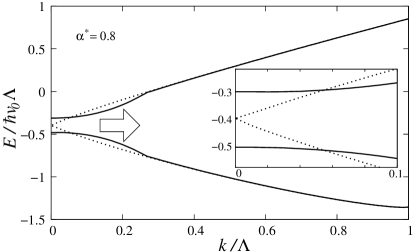
Figure 2: The dispersion law $E_{\kappa}(k)$ in the in-plane (dashed curves) and out-of-plane (solid curves) phases for $\alpha^{*}=0.8$ corresponding to $\mathrm{SiO_{2}}$ substrateJang et al. (2008). The curves for both phases coincide for momenta larger than a certain critical value where $\vartheta_{k}=\pi/2$ becomes independent of $k$, see Fig. 1. The inset shows the gap region in detail.

Zero-field Hall current. To describe the Hall conductivity due to skew scattering we utilize the semiclassical Boltzmann approach which allows a physically transparent interpretation of this mechanismSinitsyn (2008); Sinitsyn et al. (2007). In general the anomalous Hall conductivity contributions can be classified by their mechanism: (i) The intrinsic contribution is due to the anomalous velocity of carriers (being non-diagonal with respect to the band index Trushin and Schliemann (2008)) which is coupled to the equilibrium part of the distribution function. (ii) The side-jump contribution follows from coordinate shifts during scattering events. It occurs in the non-equilibrium part of the distribution function as well as in the anomalous velocitySinitsyn (2008); Sinitsyn et al. (2007). (iii) The skew scattering contribution is independent of the coordinate shift and of the anomalous velocity. It occurs when the scattering rate is asymmetric with respect to the initial and final states and, therefore, must be considered beyond the first Born approximation The first two conductivity contributions do not depend on disorder but on the out-of-plane angle $\vartheta_{k}$ and can be adopted from Sinitsyn et al. (2007). Here, we focus on the skew scattering contribution which can be described using the interband incoherent Boltzmann equation where the anomalous velocity is neglected but the scattering probability is calculated up to the third order in the short-range scattering potential with the momentum-independent Fourier transform $V$. In linear order in the homogeneous electric field ${\mathbf{E}}$ this equation reads $-e{\mathbf{E}}\mathbf{v}_{k}\left[-\partial f^{0}(E_{k})/\partial E_{k}\right]=I[f^{1}_{k}]$, where $f^{0}(E_{k})$ is the Fermi-Dirac function, $f^{1}_{\mathbf{k}}$ is the non-equilibrium addition, and $\mathbf{v}_{k}$, $E_{k}$ are given by Eqs. (6,5) with $\kappa=+$. The collision integral can be written as $I[f^{1}_{\mathbf{k}}]=\int\frac{d^{2}k^{\prime}}{(2\pi)^{2}}w_{\mathbf{k}\mathbf{k^{\prime}}}(f^{1}_{\mathbf{k^{\prime}}}-f^{1}_{\mathbf{k}})$ with $w_{\mathbf{k}\mathbf{k^{\prime}}}$ being the scattering probability. We divide $w_{\mathbf{k}\mathbf{k^{\prime}}}$ into two parts. The first one is proportional to the cosine of the scattering angle and calculated up to the second order in $V$. The second one is proportional to the sine of the scattering angle and calculated up to the third order in $V$. These two parts correspond to the conventional and skew scattering respectively which can be alternatively expressed in terms of the momentum relaxation times, cf. Ref.Sinitsyn et al. (2006)

$$(\tau_{\parallel}^{\nu})^{-1}=n_{i}kV^{2}(1+3\cos^{2}\vartheta_{k}^{\nu})/(4\hbar^{2}v_{k}),$$

$$(\tau_{\perp}^{\nu})^{-1}=\nu n_{i}k^{2}V^{3}\cos\vartheta_{k}^{\nu}\sin^{2}\vartheta_{k}^{\nu}/(8\hbar^{3}v_{k}^{2}).$$ (7)

Here, $n_{i}$ is the concentration of such scatterers. Since $\tau_{\perp}^{\nu}\propto 1/V^{3}$ whereas $\tau_{\parallel}^{\nu}\propto 1/V^{2}$ it is natural to assume $\tau_{\perp}^{\nu}\gg\tau_{\parallel}^{\nu}$, and the Hall conductivity for a given valley can be estimated as $\sigma_{yx}^{\nu}\approx\sigma_{xx}\tau_{\parallel}^{\nu}/\tau_{\perp}^{\nu}\mid_{k=k_{F}}$ which can vary in a quite broad but finite range because neither of $\tau$’s diverges at low doping thanks to the $k$-dependent group velocity (6). Note that $K$ and $K^{\prime}$ contribute identically to the total Hall conductivity $\sigma_{yx}=\sum_{\nu}\sigma_{yx}^{\nu}$ if the out-of-plane pseudospin polarization is opposite in the two valleys, i. e. $\vartheta_{1}$ and $\vartheta_{2}$ are assigned to $\vartheta_{k}^{+}$ and $\vartheta_{k}^{-}$ respectively, and the time reversal invariance is broken by the exchange interactions. On the other hand, if the out-of-plane pseudospin polarization is the same in both valleys (i. e. either of $\vartheta_{1,2}$ is assigned to both $\vartheta_{k}^{\pm}$ breaking the parity invariance) the Hall currents in the two valleys have opposite directions resulting in the valley Hall effectXiao (2001) — another analog of the well known spin Hall effectSinitsyn et al. (2006).

Interband optical absorption. From $H^{\nu}_{0}$ one can deduce the following interaction Hamiltonian between the electromagnetic wave and carriers in graphene $H^{\nu}_{\mathrm{int}}=\frac{ev_{0}}{c}(\nu\sigma_{x}A_{x}+\sigma_{y}A_{y})$ which couples the vector potential $\mathbf{A}$ and pseudospin $\vec{\sigma}$. As consequence, the inter-band transition matrix elements turn out to be sensitive to the light polarization and pseudospin orientations in the initial and final states. To be specific we assume monochromatic light of frequency $\omega$, normal incidence (i.e. zero momentum transfer from photons to electrons), and circular polarization (fulfilling $A_{x}=\pm iA/\sqrt{2}$, $A_{y}=A/\sqrt{2}$). The probability to excite an electron from the valence band to an unoccupied state in the conduction band can be calculated using the golden-rule. Finally, the absorption $P^{\nu}$ can be calculated as a ratio between the total electromagnetic power $W_{a}$ absorbed by graphene per unit square and the incident energy flux $W_{i}=\omega^{2}A^{2}/4\pi c$. Then, the optical absorption for $K$ valley ($\nu=+$) reads

$$P^{+}=\frac{\pi e^{2}}{\hbar c}\frac{4\Lambda v_{0}}{\omega}\int\limits_{0}^{\infty}dxx\left\{\begin{array}[]{c}\sin^{4}\frac{\vartheta_{k}^{+}}{2}\\ \cos^{4}\frac{\vartheta_{k}^{+}}{2}\end{array}\right\}\delta\left(\frac{E_{+}-E_{-}-\hbar\omega}{\hbar v_{0}\Lambda}\right),$$ (8)

where the multipliers $\sin^{4}(\vartheta_{k}^{+}/2)$ and $\cos^{4}(\vartheta_{k}^{+}/2)$ are for two opposite helicities of light, and for K’-valley they are interchanged. If the out-of-plane pseudospin polarization is chosen to be opposite in the two valleys, then the total absorption $P=\sum_{\nu}P^{\nu}$ at small $k/\Lambda$ turns out to be sensitive to the helicity of light: It is substantially reduced for one and facilitated for another. Moreover changing the excitation energies $\hbar\omega$ we can investigate the dependence $\vartheta(k)$ shown in Fig. 1. If the out-of-plane pseudospin polarization is chosen to be the same in both valleys, then the total absorption does not depend on the radiation helicity but the two valleys turn out to be differently occupied by the photoexcited carriers which is interesting effect on its ownXiao (2001). In the in-plane phase with $\vartheta=\pi/2$ the total absorption does not depend on light polarization, and in the non-interacting limit it equals to the universal value $\frac{\pi e^{2}}{\hbar c}$, as expectedNair et al. (2008).

Conclusions. We have demonstrated that the pseudospin being until now rather uncontrollable and almost unmeasurable quantity can be “unfrozen” by the exchange electron-electron interactions (1) and play an essential role in optical and transport properties of graphene. We hasten to say that the Hartree-Fock approximation employed here has generically a tendency to overestimate ordering such as the pseudospin out-of-plane polarization. We believe, however, that the pseudospin eigenstates $|\chi_{\kappa k}^{\nu}\rangle$ derived above are much more robust because their special pseudospin-momentum entangled structure stems from the free Hamiltonian $H^{\nu}_{0}$, and the electron-electron interactions do only modify it making our predictions reliable at the qualitative level. From this point of view the pseudospin can be seen as an additional degree of freedom similar to the true spin but unaffected by the magnetic field directly. Having this similarity in mind one can think about pseudospin ferromagnetismMin et al. (2008), pseudospin accumulation at the sample’s edge by means of the zero-field Hall current, pseudospin selectivity in the optical absorption (8), and, probably, pseudospin filtering and switching. In a more distant future one can imagine some useful effects based on the pseudospin polarization like an all-electrical counterpart for GMR which is obviously very promising for application. This Letter should be seen as a first step in this direction.

This work was supported by DFG via GRK 1570.

References

- Novoselov et al. (2005) K. S. Novoselov et al., Nature 438, 197 (2005).
- Geim and Novoselov (2007) A. K. Geim and K. S. Novoselov, Nat. Mat. 6, 183 (2007).
- Castro Neto et al. (2009) A. H. Castro Neto et al., Rev. Mod. Phys. 81, 109 (2009).
- Kane and Mele (2005) C. L. Kane and E. J. Mele, Phys. Rev. Lett. 95, 226801 (2005), R. Winkler and U. Zülicke, Phys. Lett. A 374, 4003 (2010).
- Mecklenburg and Regan (2011) M. Mecklenburg and B. C. Regan, Phys. Rev. Lett. 106, 116803 (2011).
- Jang et al. (2008) C. Jang et al., Phys. Rev. Lett. 101, 146805 (2008).
- Martin et al. (2008) J. Martin et al., Nat. Phys. 4, 144 (2008), E. H. Hwang, B. Y.-K. Hu, and S. Das Sarma, Phys. Rev. Lett. 99, 226801 (2007), S. V. Kusminskiy et al., ibid. 100, 106805 (2008).
- Peres et al. (2005) N. M. R. Peres, F. Guinea, and A. H. Castro Neto, Phys. Rev. B 72, 174406 (2005).
- Barlas et al. (2007) Y. Barlas et al., Phys. Rev. Lett. 98, 236601 (2007).
- Nilsson et al. (2006) J. Nilsson et al., Phys. Rev. B 73, 214418 (2006).
- Min et al. (2008) H. Min et al., Phys. Rev. B 77, 041407 (2008), F. Zhang et al., ibid. 81, 041402 (2010), J. Jung, F. Zhang, and A. H. MacDonald, ibid. 83, 115408 (2011), J. Jung, et al., Phys. Rev. Lett. 106, 156801 (2011).
- Nagaosa et al. (2010) N. Nagaosa et al., Rev. Mod. Phys. 82, 1539 (2010).
- Sinitsyn (2008) N. A. Sinitsyn, J. Phys. Cond. Matt. 20, 023201 (2008).
- Sinitsyn et al. (2006) N. A. Sinitsyn et al., Phys. Rev. Lett. 97, 106804 (2006).
- Sinitsyn et al. (2007) N. A. Sinitsyn et al., Phys. Rev. B 75, 045315 (2007).
- (16) W.-K. Tse et al., arxiv:1101.2042.
- Orlita and Potemski (2010) M. Orlita and M. Potemski, Semicond. Sci. and Tech. 25, 063001 (2010).
- Bonaccorso et al. (2010) F. Bonaccorso et al., Nat. Photon. 4, 611 (2010).
- Nair et al. (2008) R. R. Nair et al., Science 320, 1308 (2008), A. B. Kuzmenko et al., Phys. Rev. Lett. 100, 117401 (2008), K. F. Mak et al., ibid. 101, 196405 (2008), E. G. Mishchenko, ibid. 103, 246802 (2009), N. M. R. Peres, R. M. Ribeiro, and A. H. Castro Neto, ibid. 105, 055501 (2010), F. T. Vasko, Phys. Rev. B 82, 245422 (2010), K. F. Mak, J. Shan, and T. F. Heinz, arxiv:1012.2922.
- Juri and Tamborenea (2008) L. O. Juri and P. I. Tamborenea, Phys. Rev. B 77, 233310 (2008).
- Khveshchenko (2001) D. V. Khveshchenko, Phys. Rev. Lett. 87, 246802 (2001).
- Trushin and Schliemann (2008) M. Trushin and J. Schliemann, Europhys. Lett. 83, 17001 (2008), Phys. Rev. Lett. 99, 216602 (2007)
- Xiao (2001) D. Xiao et al., Phys. Rev. Lett. 99, 236809 (2007).