The Spitzer Extragalactic Representative Volume Survey (SERVS):
The Environments of High-$z$ SDSS Quasi-Stellar-Objects

Abstract

This paper presents a study of the environments of SDSS Quasi-Stellar-Objects (QSOs) in the Spitzer Extragalactic Representative Volume Survey (SERVS). We concentrate on the high-redshift QSOs as these have not been studied in large numbers with data of this depth before. We use the IRAC $3.6$-$4.5\mu$m colour of objects and ancillary $r$-band data to filter out as much foreground contamination as possible. This technique allows us to find a significant ($>4$-$\sigma$) over-density of galaxies around QSOs in a redshift bin centred on $z\sim 2.0$ and a ($>2$-$\sigma$) over-density of galaxies around QSOs in a redshift bin centred on $z\sim 3.3$. We compare our findings to the predictions of a semi-analytic galaxy formation model, based on the $\Lambda$CDM millennium simulation, and find for both redshift bins that the model predictions match well the source-density we have measured from the SERVS data.

1. Introduction

The Spitzer Extragalactic Representative Volume Survey (SERVS; Mauduit et al. 2011, in prep) is a warm Spitzer survey at $3.6$ and $4.5\mu$m which will cover an area of 18 deg² in fields already extremely well-studied and hence with a large amount of ancillary data. The survey reaches depths of $\sim 1\,\mu$Jy allowing $L_{*}$ galaxies to be observed out to $z\sim 5$, thus making it ideal for studying the environments in which AGN reside out to these epochs.

It is now widely accepted that high-luminosity active galactic nuclei (AGN) harbour accreting super-massive black holes with masses of the order $10^{7-9}\mbox{\,$\rm M_{\odot}$}$, implying that their host galaxies are amongst the most massive in existence at their respective epochs. Indeed, many studies have now shown that the most luminous types of AGN preferentially reside within fields containing over-densities of galaxies (e.g. Hall & Green 1998; Best et al. 2003; Wold et al. 2003; Hutchings et al. 2009) as would be expected of the most massive galaxies at any epoch. These points support the idea that luminous AGN can be utilised as signposts to extreme regions of the dark matter density and thus the most massive dark matter haloes (e.g. Pentericci et al. 2000; Ivison et al. 2000; Stevens et al. 2003) at high-redshift. Combining this technique with large multiwavelength surveys, like the Sloan Digital Sky Survey (SDSS; Abazajian et al. 2009) which has identified more than 120000 broad-line quasi-stellar objects (QSOs) up to some of the highest measured redshifts (i.e. $z$=6.4, Fan et al. 2003; Willott et al. 2003) has opened up a new era in AGN research.

Recently the Spitzer Space telescope has been at the forefront of this work due to its currently unique sensitivity to hot dust, which is an important component of most AGN unified theories (Antonucci, 1993). It has also been utilised in the search for high-redshift galaxy clusters (e.g. Eisenhardt et al. 2008, Wilson et al. 2009, Papovich et al. 2010). Its wavelength range, particularly that of the Infrared Array Camera (IRAC; Fazio et al. 2004), provides the necessary extension needed to take cluster finding techniques to $z>1$. Indeed it has led to the highest known spectroscopically confirmed cluster to date (Papovich et al. 2010; Tanaka et al. 2010) at $z=1.62$, found solely from an over-density of IRAC sources in the XMM-LSS field of the Spitzer Wide-Area Infrared Extragalactic (SWIRE; Lonsdale et al. 2003) survey. Many of these methods make use of the colour space that IRAC provides since it offers a useful way to select those galaxies that are most likely to be at high-redshift. In addition, the negative k-correction caused by the 1.6 $\mu$m peak in stellar emission moving into the mid-infrared waveband means that IRAC can efficiently reach the depths required to study the high-redshift universe in technically achievable exposure times.

These features that have proved so useful for cluster finding are also very useful for the study of the environments of AGN at high-$z$. Recently in Falder et al. (2010) over-densities were found at $z\sim 1$ in IRAC data around a large sample of SDSS QSOs and radio galaxies; it was also found that radio-loud AGN reside in, on average, denser environments. The depth of these observations allowed for the detection of a $\sim 0.7L_{*}$ galaxy at the redshift of the AGN ($z\sim 1$) and we could have detected an $L_{*}$ galaxy at $z\sim 2$. On the other hand, SERVS will allow the detection of $L_{*}$ galaxies at $z\sim 5$, see Fig. 1. The main difference in the sample used by Falder et al. (2010) and the sample used in this paper is that SERVS is a blank-field rather than a targeted survey. This means the sample of AGN is selected due to being in the survey region rather than based on other criteria related to the AGN. Hence, we will not have a sufficient number of powerful radio-loud AGN to look for similar effects as seen in Falder et al. (2010) because these are rare and require large areas or snapshot surveys to study in large numbers. However, the almost unrivalled combination of depth and area that SERVS provides will allow us to see if luminous AGN in general are found in over-densities at $z>>1$.

Figure 1.— The limiting magnitudes in terms of $L_{*}$ versus redshift for the INT $r$-band data (dashed line) as well as the SERVS $3.6{\mu}m$ and $4.5{\mu}m$ data (solid and dash-dot lines respectively). Also shown for comparison is the SWIRE survey’s $3.6{\mu}m$ data (triple-dot-dash line) and the $3.6{\mu}m$ data used in Falder et al. (2010). Full details of the models used to construct this figure are given in the text.

There is another link between the study of AGN environments and the study of high-redshift clusters. Finding clusters beyond $z\sim 1.5$ is challenging and requires large, deep sky surveys; for example Papovich et al. (2010) required all of the SWIRE survey (49 sq degrees) to locate a $z=1.62$ cluster. However, AGN are extremely luminous and therefore detectable out to $z>6$ with shallow wide surveys like the SDSS or by their radio emission in large area radio surveys. Many authors have therefore used these signposts for high-density regions in the universe for follow-up and have located high-redshift clusters and proto-clusters in observationally efficient ways (e.g., Pentericci et al. 2000, Stern et al. 2003, Venemans et al. 2007, Doherty et al. 2010, Galametz et al. 2010). At $z>3$ only a handful of these proto-clusters have been detected to date, mainly around individual radio-galaxies (e.g., Overzier et al. 2006, 2008). Recently in a study similar to this work Hatch et al. (2010) have studied the environments of $z\sim 2.4$ radio galaxies. In their work they find potential proto-clusters around three of their six targets, with good evidence that the excess objects are blue star-forming galaxies. Furthermore, studying the environments of high-redshift AGN may provide important constraints on the level of positive (e.g. Elbaz et al., 2009) or negative (e.g. Rawlings & Jarvis, 2004) AGN driven feedback on galaxies in the immediate environment of the AGN.

In this paper we take advantage of the depth of SERVS to study the environments in which high-redshift QSOs reside. The layout of the paper is as follows: in Sections 2 and 3 we discuss the observations and the sample of QSOs, in Section 4 we describe our analysis, we present our results in Section 5 before comparing them to the previous work at $z\sim 1$ in Section 6 and to models in Section 7, we then finish with a summary in Section 8. Throughout the paper we have assumed a flat cosmology with H${}_{0}=72$ km s^-1 Mpc^-1, $\Omega_{\rm{m}}=0.3$ and $\Omega_{\Lambda}=0.7$. All magnitudes are quoted in the AB system unless explicitly stated otherwise.

Figure 2.— Redshift vs rest frame optical absolute magnitude (SDSS $i$-band) for QSOs from the seventh data release of the SDSS quasar survey (Schneider et al., 2010) which are in the SERVS northern fields. The boxes show the two redshift bins we split the sample into for study as described in the text. On the right hand axis we show black-hole mass lower limits of these QSOs. These are calculated by assuming that the QSOs are accreating at the Eddington limit and using the relation from Rees (1984) with a bolometric correction factor of 15 (Richards et al., 2006) to the SDSS $i$-band absolute magnitudes.

2. Observations and Source Extraction

The primary observations used in this paper are those from the Spitzer Extragalactic Representative Volume Survey (SERVS). This is a warm Spitzer survey using IRAC channels 1 and 2 ($3.6$ and $4.5$ ${\mu}m$ respectively). The data reach approximate 5-$\sigma$ depths of $\sim 1~{}\mu$Jy (23.9 mag) at $3.6~{}{\mu}m$ and $\sim 2~{}\mu$Jy (23.1 mag) at $4.5~{}{\mu}m$. Determining the depth of a large survey is non-trivial as the coverage is not uniform in depth due to the overlaps of the scan pattern. Small areas will therefore be deeper than the average, an important consideration when measuring source density. We therefore need to cut the catalogue at a flux level which ensures equal depth throughout the maps.

Eventually SERVS will cover 18 deg² of the extremely well studied fields from the SWIRE survey. In this paper we make use of the SERVS overlap with the SDSS, thus restricting ourselves to the northern SERVS fields: Elais N1 (EN1) (1.01 deg² that overlaps the SDSS) and the Lockman Hole (4.93 deg²). Full details of the fields, observations and data reduction as well as the survey strategy will be given in Mauduit et al. (2011, in prep). In addition to the Spitzer data we make use of deep optical photometry from the INT (WFC) and KPNO (MOSAIC1), originally used by the INT WFS (McMahon et al., 2001) and the SWIRE optical imaging campaign (Lonsdale et al., 2003), but since expanded and re-reduced by Gonzalez-Solares et al. (2011, in prep). These data reach a 5-$\sigma$ depth of 24.2 mag in the $r$-band.

In Fig. 1 we show the sensitivity of the SERVS data and the $r$-band data in terms of $L_{*}$. For comparison we also show the $3.6~{}{\mu}m$ sensitivity from the SWIRE survey and that of the data used in Falder et al. (2010). The main point to note is that while SWIRE detects $L_{*}$ galaxies at $z\sim 2.5$, SERVS can detect them at $z\sim 5$. This plot was made using the restframe $K$-band luminosity function of Cirasuolo et al. (2010) assuming no evolution past $z=4$. All colour conversions between bands are derived using a Bruzual & Charlot (2003) elliptical galaxy model with reddening of $A_{v}=0.8$ applied according to the extinction law of Calzetti et al. (2000) and the hyperz software package (Bolzonella et al., 2000); this will be discussed at length in Section. 4.2. The $k$-correction is calculated using this model from Bruzual & Charlot (2003) to place SEDs at various redshifts and comparing the rest-frame and observed-frame flux in the $K$-band filter.

Figure 3.— IRAC $3.6$-$4.5\mu$m ($3.6-4.5{\mu}m$) colour vs redshift, care of the Bruzual & Charlot (2003) stellar population models and the hyperz software package (Bolzonella et al., 2000). The left panel shows the range of colours produced with six different commonly used models. These consist of a single burst model, four exponentially declining SFR models representing elliptical, S0, Sa and Sc type galaxies with $\tau$ = 1,2,3 and 15 Gyr respectively, and a model with a constant SFR (Im). All models have a formation redshift of 10 and no reddening. In the right panel we show the elliptical model without reddening and with two models with $A_{v}$ = 0.8 and 1.6 applied according to Calzetti et al. (2000). This shows that a reasonable level of reddening is likely to have more of an effect on a galaxy’s colour in this colour space than its star formation history.

The catalogue we use is the SERVS data fusion catalogue (Vaccari et al. 2011, in prep). This matches the single-band SERVS IRAC 3.6 and 4.5 $\mu$m catalogues generated with the SExtractor software package (Bertin & Arnouts, 1996), using a search radius of 1.0 arcsec, computes an average coordinate (for sources detected in both bands) and matches the resulting IRAC two-band catalogue with ancillary photometric data-sets from the far-ultraviolet to far-infrared waveband (e.g. GALEX, SDSS, CFHTCTIO/ESO/INT/KPNO/2MASS/UKIDSS/SWIRE) using a search radius of 1.5 arcsec. Since we will use the $3.6$-$4.5\mu$m colour to select sources likely to be at the correct redshift we therefore are, for the most part, restricted to using only those sources which are detected in both bands.

3. Sample

We identify QSOs in the SERVS regions by cross matching the SERVS source catalogues with the seventh data release of the SDSS quasar survey (Schneider et al., 2010) using the software package topcat (Taylor, 2005) to select the SDSS QSOs in the overlap regions. In total we find 46 QSOs in the SERVS northern fields; 5 in EN1 and 41 in the Lockman Hole. The small number in EN1 is due to the SDSS only overlapping a small portion of the observed region. These numbers include only QSOs that are at least $400$ arcsec from the edges of the regions of equal coverage in both the ch1 and ch2 images. This allows us to study the environments out to these distances without any effects from the image edges. The distribution of the sample in the L-z plane is shown in Fig. 2. Six of the lower redshift QSOs are detected by the FIRST radio survey (Becker et al., 1995) at 1.4GHz.

4. Analysis

4.1. Radial search stacking

To study the QSO environments we have employed the relatively simple technique used in Best et al. (2003) and Falder et al. (2010). This involves placing a series of concentric annuli around each QSO and counting the number of sources that meet our selection criteria, described in more detail later in Section 4.2. We can then plot the source density as a function of radial distance for each QSO. The annuli are kept to a fixed area as the radial distance increases to keep the Poisson noise at a similar level from bin-to-bin. The QSOs themselves are excluded from the search because including them would bias the first annulus; this is done by not counting any sources within $1$ arcsec of the QSO’s SDSS coordinates.

As we will be comparing our findings in this work to those from Falder et al. (2010) at $z\sim 1$ we aim to conduct the analysis in a similar way. In that work, two over-densities were reported, a sharp peak in the central source density within $300$ kpc of the AGN and then a lower level over-density extending out to at least $700$ kpc. This pattern has also been seen elsewhere in the literature, for example in Best et al. (2003) around powerful radio sources at $z\sim 1.6$, and by Serber et al. (2006) for SDSS QSOs. When we look for over-densities within $300$ kpc in this sample, while many AGN appear to have an over-dense first annulus, they lack a significant detection. This is probably due to having far fewer targets in the sample. The sample used in Falder et al. (2010) contained a much larger number of AGN ($\sim$$170$) than are present in any of our redshift bins or indeed the whole sample. Falder et al. (2010) also found that it was not possible to detect the $300$ kpc scale over-density with fewer than $\sim$$40$ randomly chosen AGN, suggesting that the central peak in source density is a harder signal to detect than the larger scale over-density.

To allow for easy comparison we use annular bins with a first bin physical radius of $700$ kpc to match the largest search radius possible in the Falder et al. (2010) data, which was in turn fixed by IRAC’s field of view. To take into account the change in scale between different redshifts we adjust the angular bin sizes for each QSO based on its redshift. This means the bins are matched in terms of their physical size, where the radius of the first annulus is $700$ kpc at the redshift of the QSOs.

To achieve a statistical result we will stack together the source density of the QSOs in two coarse redshift bins using the raw number counts. To ensure we are comparing like with like in the stacking analysis we match the range in luminosity that we are sensitive to for each QSO. This is done in each redshift bin by calculating what absolute magnitude the survey flux limit represents at the highest redshift in that bin, and then adjusting the flux cut to ensure this is matched for each of the other QSOs in that bin. As an upper limit we work out what flux a $10L*$ galaxy would have at the maximum redshift of the redshift bin and apply an upper cut on sources with fluxes greater than this limit. The reason for choosing $10L*$ is to ensure we are not cutting any likely associated galaxies, allowing for the significant uncertainty in the luminosity function at these high redshifts.

The reasoning for adopting this method of analysis is that at these high-redshifts other methods such as B_gq and 2 point correlation functions are difficult to calibrate correctly. The large error bars that result from the assumptions made about the luminosity function and $k$-correction at these redshifts make attaining a statistical result difficult.

4.2. Galaxy colours

Figure 4.— Histogram of the IRAC $3.6$-$4.5\mu$m ($3.6-4.5{\mu}m$) colour distribution in the SERVS source catalogues, shown for all sources (solid line), for sources with an $r$-band detection of 22.75 or fainter (dotted line), for sources with an $r$-band detection of 23.50 or fainter (dot and dashed line) and for those sources not detected in the $r$-band at all (dashed line). This figure clearly shows that most sources with $3.6$-$4.5\mu$m $>0.2$ are undetected in the $r$-band and therefore most likely to be at high-$z$, as Fig. 3 would suggest.

In order to increase our sensitivity to galaxies at the same redshifts as the QSOs we have made use of the IRAC $3.6$-$4.5\mu$m colour (i.e. ch1$-$ch2). To help decide on the correct colour cuts we have made use of the hyperz software package (Bolzonella et al., 2000) and the stellar synthesis models of Bruzual & Charlot (2003). In the left panel of Fig. 3 we show the colour of 6 commonly used models versus redshift. These are a single burst model, four exponentially decreasing star formation rate (SFR) models with timescales $\tau$=1, 2, 3 and 15 Gyr designed to represent elliptical, S0, Sa and Sc type galaxies respectively and a model with a constant SFR (Im). What is clear from Fig. 3 is that, with the exception of the burst model all the models produce a very similar $3.6$-$4.5\mu$m colour; at most the burst model differs by only 0.15 mags. In the right panel we show the effect that reddening has on the $3.6$-$4.5\mu$m colour; this is shown for the elliptical model without reddening along with two models with $A_{v}$=0.8 and 1.6, added according to the Calzetti et al. (2000) reddening law. This plot shows that adding a reasonable amount of reddening can have a bigger effect on this colour space at high-$z$ than the choice of star formation history. In all cases we have assumed a formation redshift for the models of $z$=10. Changing this to $z$=100 made virtually no difference, and although using $z$=5 does make a difference, at most it makes the colour bluer by $\sim$0.1 magnitudes at high-$z$. The key thing to note is that for $z>1.3$ this colour space provides a good method for selecting galaxies most likely to be at high-redshift.

Since our sample spans a range of $0.3<z<5.3$ we apply different colour cuts to encompass different parts of the sample. Where we interpret our results in terms of $L_{*}$ we use the elliptical model with $A_{v}=0.8$ (see Fig. 1). However, for our colour cuts on the data we experiment with colours that would fit any of the models. There are several factors to consider here, firstly the real colours of galaxies will contain significant scatter. We only show two parameters that can scatter the colours, SF history and extinction, but in reality there will be more, not to mention the intrinsic scatter from measurement errors. In Papovich (2008) the scatter of the $3.6$-$4.5\mu$m colour was shown by over-plotting data with spectroscopic redshifts on to the model predictions; this was possible for $z<3$ and it showed that there was a minimum of 0.2 mags of scatter at all redshifts. An especially problematic feature that Papovich (2008) reported was a population of galaxies at $z\sim 0.5$ with a significantly redder colour than could be predicted by any model or with reddening. These galaxies will certainly contaminate the colour space predicted to be occupied by high-$z$ galaxies. These issues create problems as encompassing a range of 0.4 magnitudes of colour space will mean we include a large foreground contamination, potentially washing out the signal from the high-$z$ galaxies we are interested in finding. It may prove correct that we are more sensitive to galaxies at the redshifts of interest by using a narrower region of colour space which, while losing some galaxies at the correct redshift, means we remove more contamination. The distribution of IRAC $3.6$-$4.5\mu$m colour from the SERVS source catalogues is shown in Fig. 4. When compared to Fig. 3 the spread of colours is reassuringly similar.

We therefore need a way of optimising our colour cut criterion for each redshift range. Ideally this would be done using a spectroscopic sample of galaxies which are in the SERVS fields, similar to that used by Papovich (2008). We could then use different criteria and see which values return the most galaxies at the redshift of interest compared to other redshifts. However, the number of spectroscopic redshifts available in the SERVS fields, or in general at these high-redshifts, is insufficient for this type of analysis. Instead, we conducted a Monte-Carlo simulation to adjust the colour-cut criteria used around the QSOs. This method allows both the upper and lower colour cut to be adjusted in steps within ranges determined from Fig. 3. We then measured the source density for each Monte-Carlo run and adopted the colour cut which gave us the largest over-density with respect to the background. This works on the assumption that the signal will peak when we include the most galaxies associated with the QSOs compared to contaminating galaxies. To get an idea of the probability that these over-densities are real, and not just noise spikes, we can then conduct the same experiment many times around randomly chosen locations in the SERVS maps, avoiding the locations of the QSOs in our sample.

The inability to effectively remove foreground contamination with this colour space for $z<1.3$ makes the sub-sample at these redshifts harder to study with this method. At these low redshifts the available ancillary data are able to provide a better means to study environments using photometric redshifts or alternative colour cuts. It is for this reason that in this paper we avoid the lowest redshift part of the sample. There are also far larger studies of such objects’ environments already in the literature (for example Yee & Green 1987, McLure & Dunlop 2001, Wold et al. 2001, Kauffmann et al. 2008, and with Spitzer in Falder et al. 2010) and so we feel a study with the small number we have in this sample would add little to the work already done at these relatively low redshifts. In contrast, the environments of high-$z$ QSOs have not been well studied in large numbers or with data of this depth before.

4.3. Ancillary data cuts

In addition to the IRAC colour cut discussed in Section 4.2 we use the $r$-band data from the INT (which reaches a 5-$\sigma$ limiting magnitude of 24.2) to cut as much additional foreground contamination as possible. This will hopefully allow us to tackle to some degree the $z\sim 0.5$ galaxies mentioned previously, that contaminate the colour space of higher-$z$ galaxies. The effect of cutting all sources with an $r$-band detection on the $3.6$-$4.5\mu$m colour space is shown in Fig. 4. The cut has the clear effect of removing around two thirds of the sources with a negative $3.6$-$4.5\mu$m colour, which is consistent with Fig. 3 suggesting that these sources have $z<1.5$. The other interesting feature is that very few sources with $3.6$-$4.5\mu$m $>0.2$ are detected in the $r$-band, which is again consistent with Fig. 3, suggesting that these sources are likely to lie at $z>3$.

Figure 5.— The mean completeness fit for the IRAC ch1 data, taken as the average of the completeness in the outer few annuli, therefore away from the bright QSOs. The data points show the results from our extensive simulation and the curve is a combination of a fit to an empirical model of the form $Completeness=(S^{a})/(b+cS^{a})$ for completeness less than 0.7 and a power law for completeness greater than 0.7, described in more detail in the text.

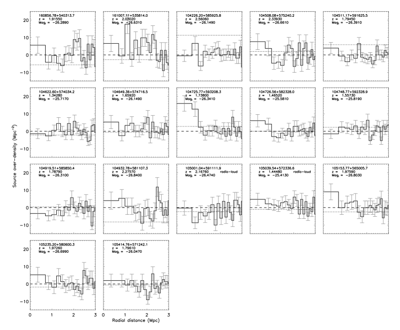
Figure 6.— Individual source over-density before being corrected for completeness vs radial distance for the 17 QSOs in the redshift range of $1.3<z<2.7$. The first bin has a radius of $700$ kpc and the other bins are of the same area as the first. The error bars show the Poisson error on the number counts. The dashed line shows the subtracted local background level (zero level) determined from an annulus of $2$ Mpc$-400$ arcsec from the QSOs. The dotted line shows, for comparison, the global background as determined from taking the average source density in large apertures over the SERVS fields. Also labelled are the QSO’s redshifts and absolute SDSS $i$-band magnitudes and those which are radio-loud.

4.4. Background level

It is important to have a measure of the background level of sources expected in the field with which to measure any over-densities against. There are several ways in which this can be done, one would be to use a systematic offset from the target and measure the source density in that region. This is known as a blank or control field and provides an estimate of the local background level. Another method when working with a large survey such as SERVS is to use a global background where the average source density of a large area or the whole survey is used. There are advantages and disadvantages to each method; using the larger area washes out any fluctuations on small scales which might affect a local value. However, if these local fluctuations are of an amplitude which makes it important to take them into account in the background determination then a local background will help if it is close enough to the target. The trade off with this method is that being too close may result in measuring the same structure of galaxies in both the background and target field.

Both methods have been experimented with in this paper. The global background has been calculated for each of the two SERVS fields, EN1 and the Lockman Hole, by placing a series of $0.5^{\circ}$ radius circles on to the catalogues and determining the average source density contained within them. The local values have been calculated by using the average source density in an annulus which is sufficiently far from the QSOs that it should not be measuring the same structure. These annuli have a maximum radius of $400$ arcsec from the QSO to ensure none of them fall off the image edges. The inner radius is determined such that it should be 2 Mpc from the QSOs at their redshift. This should be far enough that we are not likely to be measuring the same large-scale structure that the QSOs reside in. Most evidence in the literature suggests that, except for the largest galaxy groups and clusters, most of their members are found within a radius $<2$ Mpc (for example Hansen et al. 2005 and Papovich et al. 2010).

Obviously the background levels have to be determined in an identical way to how we measure the source density in the environments of the QSOs and will be a different value for each colour and $r$-band criterion that we use. The error on the background is calculated as the Poisson error on the raw number counts used for the background measurements. This is then scaled to the same area and added in quadrature to the error on the source density measurements to get the error on any over-density.

4.5. Completeness

In order to account for the incompleteness of the Spitzer data near the flux limit of the survey we ran an extensive completeness simulation. This largely followed the process used in Falder et al. (2010) and full details are given there. It involved cutting out regions of the Spitzer images surrounding each QSO that measured $900\times 900$ arcsec, i.e., large enough to include all annuli used in our analysis. We then inserted 10000 artificial sources into each of these cut outs for 40 different flux levels. To avoid increasing source confusion these were added in batches of 1000 which meant that they were never too close together that they could become confused with another artificial source. At each flux level we compared the number of inserted sources to those found in the source catalogues. We consider a source recovered if it is found within $1.2$ arcsec (2 pixels) of the inserted location and within a factor of 2 of the inserted flux. The results of this analysis are measured for each annulus separately which then enables us to apply a completeness correction specific to each annulus. This means we account for missed area in the vicinity of bright stars or indeed the QSOs. It was shown in Falder et al. (2010) that the bright QSO in the first annulus has the effect of lowering the completeness in innermost annuli.

To eliminate the scatter in the measured completeness curves we then fitted them with an empirical model of the form $Completeness=(S^{a})/(b+cS^{a})$ (Coppin et al. 2006) where $S$ is the 3.6 $\mu$m or 4.5 $\mu$m flux density and $a$, $b$ and $c$ are constants that are fitted. It was found, however, that this model alone was unable to provide a good fit at the knee between the bright end and the steep slope; the data appear less complete here than would be expected based on the S shape curve although this is at most a 10 per cent effect. It is suspected this effect is likely due to source confusion as the SERVS data are confused using the classical definition of 30 beams per source (Mauduit et al. 2011, in prep). In order to overcome this effect we instead fitted a power law to the data points when the completeness was greater than 0.70 (see Fig.5). The completeness is measured in both the $3.6\mu$m and $4.5\mu$m images. We are then able for each detected source in the real catalogues to calculate the correct completeness correction to apply by multiplying the completeness fraction corresponding to the measured $3.6\mu$m and $4.5\mu$m fluxes of the source.

We show the mean completeness curve for the $3.6\mu$m cutouts in Fig.5 based on the outer annuli, therefore away from the bright QSOs. To make a conservative cut at the 50 per cent completeness value, we use the flux density at which we are 50 per cent complete in the first annulus. This gives a mean 50 per cent completeness at $3.6\mu$m of $1.50\pm 0.11\mu$Jy ($23.46^{+0.08}_{-0.07}$) and at $4.5\mu$m of $1.77\pm 0.08\mu$Jy ($23.28^{+0.05}_{-0.05}$). To be conservative we only use sources detected with fluxes greater than the highest flux level at which any of our QSO’s first annuli were 50 per cent complete in each channel; these values are $1.71\mu$Jy (23.32) at $3.6\mu$m and $1.89\mu$Jy (23.21) at $4.5\mu$m.

5. Results

In order to have suitable numbers of objects in each redshift range we have divided the sample into two redshift bins shown in Fig. 2. The first is centred on $z\sim 2.0$ and spans the range $1.3<z<2.7$ and the second is centred on $z\sim 3.3$ and spans the range $2.8<z<3.8$. These bins were chosen since there is a natural divide in the sample at $z\sim 2.8$ which gives samples of 11 and 17 QSOs in the two bins. This is a trade off between having enough QSOs in the sub-samples whilst restricting the sample to as small a fraction of cosmic time as is possible. As mentioned earlier for QSOs with $z<1.3$ the colour space is contaminated by lower redshift galaxies and these are already better studied in the literature. We also looked at the two $z\sim 5$ QSOs but failed to gain a significant detection of galaxies in their environments, which is not surprising for such a small sample.

5.1. $z\sim 2.0$ sample

Table 1Table showing the set of upper and lower $3.6$-$4.5\mu$m colour criterion used for the Monte-Carlo analysis on the sample centred on $z\sim 2.0$, along with each set’s associated Poisson significance. Also shown is the percentage of times that this significance was achieved in the Monte-Carlo simulation around random points for this colour criterion. The colour criterion that gives the most significant over-density is shown in bold. The bottom two colour steps are designed for comparison to look above and below the region of colour space at which we expect to find an over-density, as would be expected these two criterion do not produce a significant over-density.

Lower cut	Upper cut	$\sigma_{Poisson}$	Monte-Carlo %
-0.30	0.10	3.22	0.50
-0.30	0.15	4.01	0.10
-0.30	0.20	3.32	0.60
-0.30	0.25	3.13	1.00
-0.30	0.30	3.18	1.00
-0.25	0.10	3.29	0.40
-0.25	0.15	4.10	0.10
-0.25	0.20	3.37	0.40
-0.25	0.25	3.17	0.80
-0.25	0.30	3.21	0.80
-0.20	0.10	3.23	0.40
-0.20	0.15	4.08	0.00
-0.20	0.20	3.29	0.50
-0.20	0.25	3.07	1.00
-0.20	0.30	3.12	1.20
-0.15	0.10	2.60	1.20
-0.15	0.15	3.56	0.20
-0.15	0.20	2.72	1.80
-0.15	0.25	2.50	3.10
-0.15	0.30	2.56	3.20
-0.10	0.10	2.03	3.80
-0.10	0.15	3.12	0.50
-0.10	0.20	2.23	4.30
-0.10	0.25	2.00	7.41
-0.10	0.30	2.08	7.01
-0.05	0.10	1.50	10.11
-0.05	0.15	2.76	1.00
-0.05	0.20	1.79	9.21
-0.05	0.25	1.56	13.71
-0.05	0.30	1.65	12.11
NA	-0.20	0.70	31.03
0.20	NA	-0.84	78.18

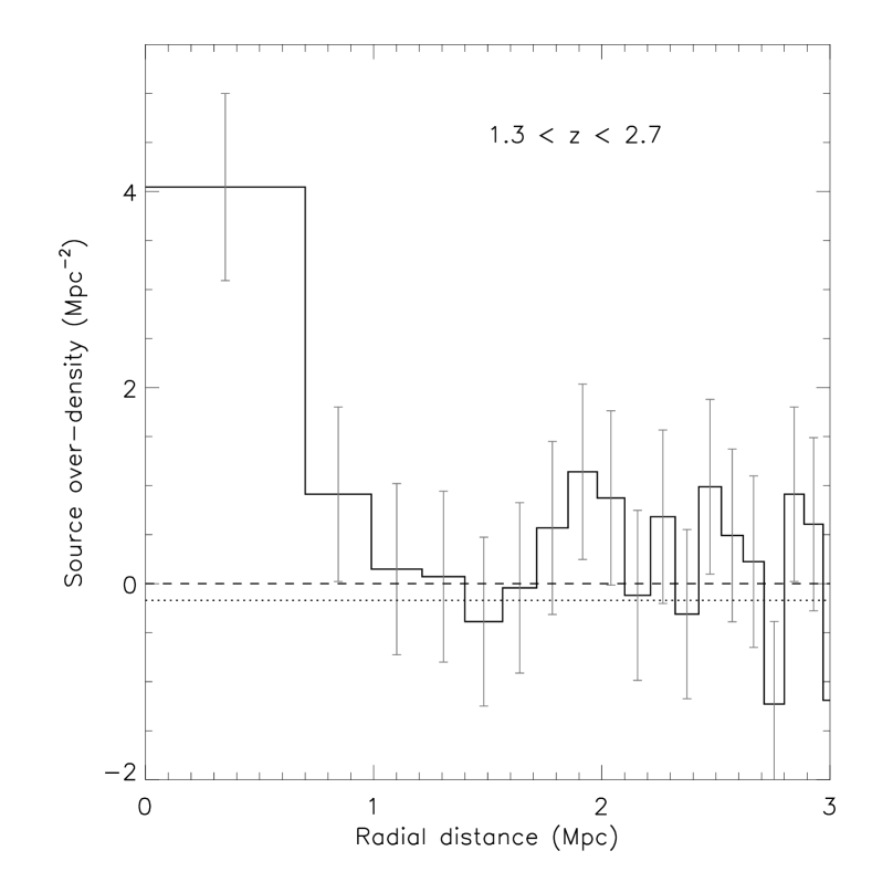
Figure 7.— Stacked source over-density before being corrected for completeness vs radial distance for the 17 QSOs in the redshift range of $1.3<z<2.7$. The first bin has a radius of $700$ kpc and the other bins are of the same area as the first. The error bars show the Poisson error on the number counts. The dashed line shows the subtracted local background level (zero level) determined from an annulus of $2$ Mpc$-400$ arcsec from the QSOs. The dotted line shows, for comparison, the global background as determined from taking the average source density in large apertures over the SERVS fields.

Figure 8.— Histograms showing the IRAC $3.6$-$4.5\mu$m colour of sources in the SERVS catalogues. In the top panel the dotted line shows the averaged local background source density surrounding the QSOs in the $z\sim 2.0$ sample and the dashed line shows the averaged source density inside the first annuli surrounding these QSOs. The bottom panel shows the result of subtracting the local background from the source density in the first annulus.

In the redshift range $1.3<z<2.7$ there are 17 QSOs of which two are detected by FIRST. These are 105001.04+591111.9 and 105039.54+572336.6 with radio luminosities of Log${}_{10}(\rm L_{1400}/\rm{W\ Hz}^{-1}\ \rm{sr}^{-1})=25.39$ and $25.16$ respectively (calculated using the FIRST radio flux and assuming a spectral index of 0.7). The flux limit at which we are 50 per cent complete at the maximum redshift of this part of the sample corresponds to an absolute magnitude of -23.4 and so we restrict our search around each QSO to galaxies brighter than this value (note that we ignore the $k$-correction within the bin as this is at most a 0.02 magnitude effect). The adopted limit represents galaxies which are roughly $0.7L_{*}$ or brighter in this redshift range.

To choose a colour criterion for this sample we use Fig. 3 to point us towards colours which may select galaxies at the redshift we are interested in. We then use our Monte-Carlo code to vary both the upper and lower colour cuts in steps within an appropriate range of model predictions. The results of this analysis are shown in Table 1 which shows that the most significant over-density of $4.10\sigma$ occurs in the stacked source density when a colour criterion of $-0.25<$ $3.6$-$4.5\mu$m $<0.15$ is used. In addition to the IRAC colour cut, we remove sources detected in the $r$-band with an apparent magnitude brighter than 23.5. This criterion corresponds to removing objects that are $\sim 4L_{*}$ or brighter according to our choice of models, meaning we are only excluding, if anything, the rarest galaxies associated with the QSOs.

The individual histograms of source over-density versus radial distance for each of these 17 QSOs are shown in Fig. 6; these show the source density with the local background level subtracted. One of these QSOs has a significant over-density around it at $>3\sigma$ level (given by Poisson statistics), while several of the other first annuli are more than 1-$\sigma$ over-dense, which suggests stacking may produce a robust signal. It is worth noting that neither of the two radio-loud QSOs (labelled) show any sign of an over-density, which means we are confident that they will not bias the stacked source-density as the results of Falder et al. (2010) suggests they might, probably due to their comparatively low radio luminosity.

The resulting stacked source density is shown in Fig. 7, which shows an over-density within $700$ kpc of the QSOs and is significantly above the local background level at the 4.10-$\sigma$ (given by Poisson statistics) level. The next annulus is also above the background level hinting that the over-density extends to around the $1$ Mpc scale. If we exclude the QSO that has an individually significant over-density this reduces to the 3.3-$\sigma$ level suggesting that the over-density we see in the stacked histogram is not just around that one object. The global background while looking consistent in most cases, seems to be too high or low in a few cases, suggesting they are in a region with a locally high or low background density. Using the global background has the effect of increasing the detected over-density to the 4.44-$\sigma$ level; we show where the global background level would be for comparison with a dotted line in Figs. 6 and 7.

To put this choice of colour cut into context we show a histogram of the $3.6$-$4.5\mu$m colour space in Fig. 8 for both the local background and the first annuli surrounding the QSOs; shown in the bottom panel is a histogram of the result of subtracting the local background from the first annulus. There is a clear over-density significant at the $4$-$\sigma$ level in the QSO fields, the location of which in this colour space is consistent with it being in the redshift range of the QSOs.

When we run our Monte-Carlo code 1000 times on batches of 17 random locations (to match the number of QSOs used) avoiding the QSO’s locations in the process, we find that we can generate similar sized over-densities only 0.1 per cent of the time in the same colour space. This increases to only 0.5 per cent of the time over all colour space sampled in this analysis (see Table 1). We are therefore confident that this over-density is real and associated with the QSOs at the 99.5 per cent confidence level using this method. The reason that this random field test does not generate Poisson statistics is that in reality galaxies are clustered, and so the probability of finding a second galaxy is not mutually exclusive of finding the first as is the case for the Poisson distribution. It is worth noting that if we apply a more simplistic colour cut $-0.25<$ $3.6$-$4.5\mu$m, to remove only foreground galaxies a 2.8-$\sigma$ (Poisson) over-density still remains.

Physically, the over-density in the first bin including a correction for completeness corresponds to, on average, 7-10 brighter than $\sim 0.7L_{*}$ galaxies, with our choice of models. This number is in excess of the local field level around each QSO within $\sim 700$ kpc, taking into account the range spanned by the 1-$\sigma$ error bars in Fig. 7.

5.2. $z\sim 3.3$ sample

Table 2Table showing the same as in Table 1 but for the sample centred on $z\sim 3.3$. This is shown both for the analysis down to the conservative 50 per cent completeness limit (c50) and the 30 per cent completeness limit (c30).

Lower cut	Upper cut	$\sigma_{c50}$	M-C %c50	$\sigma_{c30}$	M-C %c30
-0.10	0.30	0.94	28.50	1.29	23.00
-0.10	0.35	1.33	19.90	1.77	14.70
-0.10	0.40	1.36	18.80	1.83	14.00
-0.10	0.45	1.63	13.90	2.08	9.10
-0.05	0.30	1.17	22.10	1.49	19.40
-0.05	0.35	1.57	14.70	1.99	11.70
-0.05	0.40	1.60	13.50	2.05	11.30
-0.05	0.45	1.88	10.00	2.31	7.60
0.00	0.30	0.79	31.90	1.08	26.20
0.00	0.35	1.24	20.70	1.64	16.10
0.00	0.40	1.27	19.20	1.70	15.80
0.00	0.45	1.58	14.10	1.98	10.90
0.05	0.30	1.61	10.80	1.77	11.50
0.05	0.35	2.04	6.90	2.33	5.40
0.05	0.40	2.06	7.10	2.38	5.40
0.05	0.45	2.37	4.20	2.66	3.50
0.10	0.30	1.18	19.40	1.36	17.60
0.10	0.35	1.69	9.60	2.01	7.30
0.10	0.40	1.71	9.90	2.06	7.50
0.10	0.45	2.06	6.00	2.38	4.30
0.15	0.30	1.59	10.20	1.95	5.70
0.15	0.35	2.14	4.40	2.62	2.20
0.15	0.40	2.14	4.40	2.65	2.60
0.15	0.45	2.51	1.70	2.99	0.70
0.20	0.30	1.60	9.20	2.11	2.80
0.20	0.35	2.22	2.90	2.86	0.70
0.20	0.40	2.19	2.90	2.85	0.50
0.20	0.45	2.62	1.10	3.22	0.10
0.45	NA	0.46	37.80	0.23	41.70
NA	0.05	0.55	36.10	0.75	31.90

In the bin that spans the redshift range $2.8<z<3.8$ there are 11 SDSS QSOs. Using Fig. 3 we again experiment, as in Section 5.1 with our Monte-Carlo method of adjusting the colour cuts. The results of this analysis are given in Table 2 which shows that we find that a colour criterion of $0.20<$ $3.6$-$4.5\mu$m $<0.45$ provides the largest over-density. We again hope to minimise contamination from the foreground by cutting all sources detected in the $r$-band with an apparent magnitude brighter than 23.5. In this redshift range this criterion corresponds to cutting objects that are $\sim 4L_{*}$ or brighter, according to our choice of models, ensuring once again we are only excluding, if any, the rarest galaxies associated with the QSOs. The flux at which we are 50 per cent complete corresponds to an absolute magnitude of -24.4 at the maximum redshift of this samples range and so we restrict the search around each QSO to galaxies brighter than this limit (we ignore the $k$-correction within the bin as this is at most a 0.2 magnitude effect). Our adopted limit represents galaxies which are roughly $1.1L_{*}$ or brighter in this redshift range.

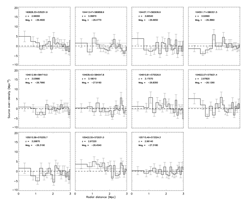
Figure 9.— Showing the individual source over-density vs radial distance for the 11 QSOs in the redshift range $2.8<z<3.8$. The first bin has a radius of $700$ kpc and the other bins are of the same area as the first. The error bars show the Poisson error on the number counts. The dashed line shows the subtracted local background level (zero level) determined from an annulus of $2$ Mpc$-400$ arcsec from the QSOs. The dotted line shows, for comparison, the global background as determined by taking the average source density in large apertures over the SERVS fields. Also labelled are the QSO’s redshifts and absolute SDSS $i$-band magnitudes. This is the source density before being corrected for completeness.

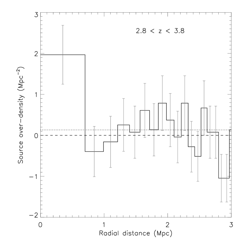
Figure 10.— Stacked source over-density vs radial distance for the 11 QSOs in the redshift range of $2.8<z<3.8$. The first bin has a radius of $700$ kpc and the other bins are of the same area as the first. The error bars show the Poisson error on the number counts. The dashed line shows the subtracted local background level (zero level) determined from an annulus of $2$ Mpc$-400$ arcsec from the QSOs. The dotted line shows, for comparison, the global background as determined from taking the average source density in large apertures over the SERVS fields. This is the source density before being corrected for completeness.

Figure 11.— Histograms showing the IRAC $3.6$-$4.5\mu$m colour of sources in the SERVS catalogues. In the top panel the dotted line shows the average local background source density surrounding the QSOs in the $z\sim 3.3$ sample and the dashed line shows the average source density inside the first annulus surrounding these QSOs. The bottom panel shows the result of subtracting the local background from the source density first annulus.

The individual histograms of source density versus radial distance for each of these 11 QSOs are shown in the top panel of Fig. 9. Though there are no statistically significant over-densities, many of the first annuli are more than 1-$\sigma$ (given by Poisson statistics) with one 2-$\sigma$ above the local background level.

The stacked source density is plotted in Fig. 10 which shows a clear peak in the source density within $700$ kpc of the QSOs. This peak is significantly above the local background at the 2.62-$\sigma$ (given by Poisson statistics). Looking at the individual histograms (Fig. 9) we again find that there is evidence to suggest that using local background subtraction is the right approach. However, using a global background in the stacking process has little affect on the result, only reducing the significance to the 2.55-$\sigma$ level. We find that if we allow our search to be slightly more sensitive by going down to the flux at which we are 30 per cent complete the stacked source density in this colour space becomes more significantly over-dense ($3.2$-$\sigma$), see Table 2. This is further evidence that the result is likely to be real since we get a stronger signal despite relaxing our conservative flux cut. We use the source-density from the 50 per cent completeness analysis for comparison to other work.

In Fig. 11, we show the $3.6$-$4.5\mu$m colour space for the local backgrounds and first annulus for this sample along with the result of subtracting the local background. There is a clear over-density at the $\sim 2.6$-$\sigma$ level in the colour range chosen. The result of this test is thus consistent with the detected over-density being at the redshift of the QSOs in this part of the sample.

When we run our Monte-Carlo code 1000 times on batches of 11 random locations, avoiding these QSOs, we find that in this colour space we can generate similar sized over-densities only 1.1 per cent of the time. If we extend this to all the colour space used in the analysis (see Table 2) then this increases to 11.9 per cent. Using the more sensitive 30 per cent completeness flux limit this improves such that in the colour space chosen we only get a $3.2$-$\sigma$ over-density 0.1 per cent of the time, and over all colour space 5 per cent of the time.

Physically this over-density with a correction for completeness corresponds to on average 2-5 brighter than $\sim 1.1L_{*}$ galaxies, with our choice of models, in excess of the local field level around each QSO within $\sim 700$ kpc.

5.3. Comparison between redshift bins

To compare our two sub-samples we re-analyse the $z\sim 2.0$ sample such that we are only sensitive to galaxies with absolute magnitudes brighter than -24.4, to match the sensitivity of the $z\sim 3.3$ sample, again neglecting the $k$-correction which is a 0.02 magnitude effect. In doing this we find 3-6 galaxies brighter $\sim L_{*}$ around the $z\sim 2.0$ sample. Hence the population of massive, brighter than $\sim L_{*}$, galaxies around the two samples seems to be comparable. This is certainly good evidence that the massive (larger than $L_{*}$) galaxies in proto-clusters are already in place by $z\sim 3$-$4$, where to date only a handful of detections have been made predominantly around individual high-$z$ radio-galaxies (e.g., Overzier et al. 2006, 2008). This picture fits in with the idea of downsizing where massive galaxies form and cluster before those of lower mass (Cowie et al. 1996; Heavens et al. 2004).

6. Comparison with previous work at ${z}\sim 1$.

In this section we compare our results to the previous work at $z\sim 1$ by Falder et al. (2010). The data for the $z\sim 1$ sample is sensitive to galaxies with an absolute magnitude of -23.0. We therefore looked again at the data from Falder et al. (2010) using a $700$ kpc annulus and restricting ourselves to flux limits which mean that we our sampling the same absolute magnitude range at $z\sim 1$ as in the samples discussed here using the SERVS data. To compare with the $z\sim 2.0$ sample in which we are sensitive to an absolute magnitude of -23.4 we apply a $k$-correction of 0.4 magnitudes and re-analyse the $z\sim 1$ data down to an absolute magnitude of -23.0. This gives 4-6 galaxies within $700$ kpc compared to the 7-12 around the $z\sim 2.0$ sample. In the $z\sim 3.3$ sample we are sensitive to galaxies with absolute magnitudes of -24.4, again applying a $k$-correction of 0.4 magnitudes we re-analyse the $z\sim 1$ data down to an absolute magnitude of -24.0. This gives 1-2 galaxies within $700$ kpc compared to the 2-5 around the $z\sim 3.3$ sample. On face value therefore it suggests that the number of galaxies around $z\sim 1$ sample is lower. This may well be the case and would fit in with the idea of downsizing of the AGN population where AGN at higher redshift are those in bigger groups or clusters than at lower redshift (Romano-Diaz et al., 2010). However it is likely that the colour selection that we use in this work means we are more efficiently removing contamination and therefore detecting a higher signal, this may go some way to explaining the difference.

7. Comparison with galaxy formation models

In this section we compare our findings with predictions from the Durham semi-analytic galaxy formation model of Bower et al. (2006), which is based on the $\Lambda$CDM millennium simulation (Springel et al., 2005). They populate the dark matter haloes created by the millennium simulation with galaxies using their semi-analytic formula, galform. The millennium simulation is an N-body simulation consisting of a box with sides of $500/h~{}$Mpc in co-moving units containing $10^{10}$ particles of mass $8.6\times 10^{8}{\mbox{\,$\rm M_{\odot}$}}/h$. The simulation started from an initial set of density perturbations at $z=127$ calculated analytically, which is then allowed to evolve under the influence of only gravity to the present day. Snapshot catalogues of the structures (dark matter haloes) that formed and merged in the box were saved at 64 epochs and it is these on to which the Durham galaxies are added. The choice of the Durham model is partly based on the fact that they give their galaxies central black-hole masses (see (Bower et al., 2006) for details), which we use to compare to our QSOs, but also because it has recently shown to be one of the best fitting models to the observed luminosity function at $z<4$ (Cirasuolo et al., 2010). However, as with all current models there are still some issues with both the faint and bright end predictions (e.g. Cirasuolo et al., 2010; Henriques et al., 2010).

In order to compare our findings with what is predicted by the Durham model we have queried the catalogues for each subset of our QSO sample. We have generated catalogues from the model which contain objects with luminosities a factor of $2$ fainter than we are sensitive to in each of the redshift ranges. This allows us to show how the predictions change if we have under or over-estimated our survey depth within a reasonable range. For each redshift range we query the model catalogues at the closest snapshot to the mid-point of the redshift range. We have then searched these catalogues for objects around galaxies with black-hole masses greater than three different values ($M_{bh}>$$10^{8.50}$, $10^{8.75}$ and $10^{9.0}\mbox{\,$\rm M_{\odot}$}$).

This procedure should replicate as closely as possible what we have done with the SDSS QSOs in SERVS, as by observing the fields around luminous high-$z$ QSOs we know we are centring on large black-holes at the redshift of the QSO. It is not currently possible for most of our sample to measure the black-hole masses using virial methods as even the Mgii  line moves out of the SDSS spectral range at $z=2.25$. However, we know that these high luminosity QSOs must be hosted by some of the largest black-holes at any given epoch. One way to quantify this is through using Eddington arguments to place lower limits on the black-hole masses of our QSOs. Using the SDSS absolute $i$-band magnitude with a bolometric correction of 15 (Richards et al., 2006) we can make the assumption that the QSOs are accreting at the Eddington limit and so their bolometric luminosity is equal to their Eddington luminosity. This then allows us to place a lower limit on the mass of black-hole required to power each QSO, using the relationship between Eddington luminosity and black-hole mass from Rees (1984). We present the results of this analysis on the right-hand axis of Fig. 2 showing the range of black-hole mass lower limits for each part of the sample. It is worth noting that there are no black-holes in the model at $z\sim 3.3$ that have a mass $>10^{9.25}\mbox{\,$\rm M_{\odot}$}$, hence why we didn’t extend the range of black holes we searched around to better match our range in Fig. 2.

We are able to query the full simulation box for the higher redshift part of our sample, but for the lower redshift part we have to restrict the volume queried to a $350/h$ Mpc on a side box due to the time restriction on queries. This is not an issue, however, because at lower redshift the population of large black holes is, as would be expected, higher and so we require less area to find the same number of suitable targets. As the longest wavelength that the model produces is the $K$-band we use our modelled $K-3.6{\mu}m$ colour from Section 4.2 to match to our observations. To account for the effect of in reality measuring counts in a cylinder we search within our physical search radius of $700$ kpc in two dimensions of the simulation and then within $3$ Mpc in the third dimension. This effect as described in Yee & Ellingson (1995) increases the sources detected by a factor of $\sim$1.5. We can then compare the measured over-density, which we assume is all associated with the QSOs, to the number of comparable galaxies we find in the model catalogues within the same radius.

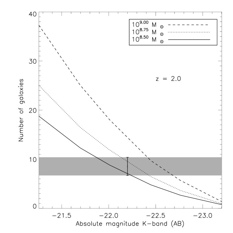
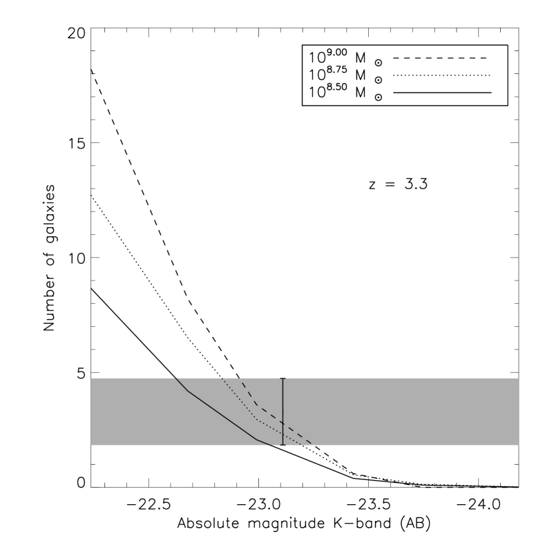
Figure 12.— The left panel shows the comparison of the $1.3<z<2.7$ sample to the Durham model, the right panel shows the same but for the $2.8<z<3.8$ sample. The grey shaded band shows the 1-$\sigma$ error on the number of galaxies we have found surrounding our QSOs in each case, and the error bars show where we estimate we have reached down to on the galaxy luminosity function. These numbers are completeness corrected. The lines then show the number of galaxies predicted by the model within the same radius with three different masses for the central galaxy’s black-hole mass (where the solid, dot, and dashed lines represent $10^{8.50}$, $10^{8.75}$ and $10^{9.0}\mbox{\,$\rm M_{\odot}$}$ black-holes respectively).

The results of this comparison are shown in Fig. 12. The grey shaded band shows the 1-$\sigma$ error on the number of galaxies we have found surrounding our QSOs in each case, and the error bar shows where we estimate we have reached down to in terms of galaxy absolute magnitude with our analysis. The lines then show the number of galaxies predicted by the model within the same cylindrical search area for galaxies with three different central black-hole masses.

Interestingly, in both cases we find that our detected source density matches well with the predictions of the models. In the $z\sim 2.0$ redshift bin the model predictions for the $10^{8.50}$ and $10^{8.75}\mbox{\,$\rm M_{\odot}$}$ black-holes fall within the $1$-$\sigma$ error bars of our measured source density. In the $z\sim 3.3$ redshift bin the model predictions for the $10^{8.75}$ and $10^{9.00}\mbox{\,$\rm M_{\odot}$}$ black-holes fall within the $1$-$\sigma$ error bars of our measured source density. It is worth noting that in our estimates of the black-hole masses of our sample the $z\sim 3.3$ part of the sample has on average larger black-hole masses due to its on average higher luminosity.

8. Summary

In this paper we have undertaken a study of the environments of SDSS QSOs in the deep SERVS survey using data from Spitzer’s IRAC instrument at $3.6~{}{\mu}m$ and $4.5~{}{\mu}m$. We concentrate our study on the high-redshift QSOs as these have not previously been studied with statistically large samples or with data of this depth. These are highly luminous QSOs $M_{i}\lesssim-26$ and hence harbour massive black-holes $M_{bh}\gtrsim 10^{8}\mbox{\,$\rm M_{\odot}$}$. In contrast, the environments of lower redshift QSOs have been studied in detail with much larger samples (Falder et al., 2010). We split the $z>1$ QSOs up into two sub-samples depending on their redshift, this allows us to apply different source selection criteria to each sample. The criteria we apply are a combination of an IRAC $3.6$-$4.5\mu$m colour selection and a cut of sources detected above a certain brightness in the the ancillary $r$-band data from the INT.

Using this method we are able to detect a significant ($>4$-$\sigma$) over-density of galaxies around the QSOs in the sub-sample centred on $z\sim 2.0$ and ($>2$-$\sigma$) in the sub-sample centred on $z\sim 3.3$, providing furthur evidence that high luminosity AGN can be used to trace clusters and proto clusters at these epochs. We compare the number counts of $L_{*}$ or brighter galaxies around each sample and find them to be comparable, suggesting the massive galaxies in proto-clusters are in place by $z\sim 3-4$ which is consistent with the idea of downsizing. We then compare these findings to those of Falder et al. (2010) at $z\sim 1$ and find that the over-densities found in this work are slightly larger than those found in Falder et al. (2010). However it is likely that the colour selection used in this work allows for a more efficient detection of possible companion galaxies and therefore this difference may well not be a real effect.

We then compare our results to the predictions from the Durham (Bower et al., 2006) galaxy formation model, built on top of the Millennium simulation (Springel et al., 2005) dark matter halo catalogues. In both cases we find the model predictions are within the $1$-$\sigma$ error bars of our measured source density.

References

- Abazajian et al. (2009) Abazajian, K. N., et al. 2009, ApJS, 182, 543
- Antonucci (1993) Antonucci, R. 1993, ARA&A, 31, 473
- Becker et al. (1995) Becker, R. H., White, R. L., & Helfand, D. J. 1995, ApJ, 450, 559
- Bertin & Arnouts (1996) Bertin, E., & Arnouts, S. 1996, A&AS, 117, 393
- Best et al. (2003) Best, P. N., Lehnert, M. D., Miley, G. K., & Röttgering, H. J. A. 2003, MNRAS, 343, 1
- Bolzonella et al. (2000) Bolzonella, M., Miralles, J., & Pelló, R. 2000, A&A, 363, 476
- Bower et al. (2006) Bower, R. G., Benson, A. J., Malbon, R., Helly, J. C., Frenk, C. S., Baugh, C. M., Cole, S., & Lacey, C. G. 2006, MNRAS, 370, 645
- Bruzual & Charlot (2003) Bruzual, G., & Charlot, S. 2003, MNRAS, 344, 1000
- Calzetti et al. (2000) Calzetti, D., Armus, L., Bohlin, R. C., Kinney, A. L., Koornneef, J., & Storchi-Bergmann, T. 2000, ApJ, 533, 682
- Cirasuolo et al. (2010) Cirasuolo, M., McLure, R. J., Dunlop, J. S., Almaini, O., Foucaud, S., & Simpson, C. 2010, MNRAS, 401, 1166
- Coppin et al. (2006) Coppin, K., et al. 2006, MNRAS, 372, 1621
- Cowie et al. (1996) Cowie, L. L., Songaila, A., Hu, E. M., & Cohen, J. G. 1996, AJ, 112, 839
- Doherty et al. (2010) Doherty, M., et al. 2010, A&A, 509, A83
- Eisenhardt et al. (2008) Eisenhardt, P. R. M., et al. 2008, ApJ, 684, 905
- Elbaz et al. (2009) Elbaz, D., Jahnke, K., Pantin, E., Le Borgne, D., & Letawe, G. 2009, A&A, 507, 1359
- Falder et al. (2010) Falder, J. T., et al. 2010, MNRAS, 405, 347
- Fan et al. (2003) Fan, X., et al. 2003, AJ, 125, 1649
- Fazio et al. (2004) Fazio, G. G., et al. 2004, ApJS, 154, 10
- Galametz et al. (2010) Galametz, A., Stern, D., Stanford, S. A., De Breuck, C., Vernet, J., Griffith, R. L., & Harrison, F. A. 2010, A&A, 516, A101
- Hall & Green (1998) Hall, P. B., & Green, R. F. 1998, ApJ, 507, 558
- Hansen et al. (2005) Hansen, S. M., McKay, T. A., Wechsler, R. H., Annis, J., Sheldon, E. S., & Kimball, A. 2005, ApJ, 633, 122
- Hatch et al. (2010) Hatch, N. A., et al. 2010, MNRAS, 1702
- Heavens et al. (2004) Heavens, A., Panter, B., Jimenez, R., & Dunlop, J. 2004, Nature, 428, 625
- Henriques et al. (2010) Henriques, B., Maraston, C., Monaco, P., Fontanot, F., Menci, N., De Lucia, G., & Tonini, C. 2010, ArXiv e-prints
- Hutchings et al. (2009) Hutchings, J. B., Scholz, P., & Bianchi, L. 2009, AJ, 137, 3533
- Ivison et al. (2000) Ivison, R. J., Dunlop, J. S., Smail, I., Dey, A., Liu, M. C., & Graham, J. R. 2000, ApJ, 542, 27
- Kauffmann et al. (2008) Kauffmann, G., Heckman, T. M., & Best, P. N. 2008, MNRAS, 384, 953
- Lonsdale et al. (2003) Lonsdale, C. J., et al. 2003, PASP, 115, 897
- McLure & Dunlop (2001) McLure, R. J., & Dunlop, J. S. 2001, MNRAS, 321, 515
- McMahon et al. (2001) McMahon, R. G., Walton, N. A., Irwin, M. J., Lewis, J. R., Bunclark, P. S., & Jones, D. H. 2001, New A Rev., 45, 97
- Overzier et al. (2008) Overzier, R. A., et al. 2008, ApJ, 673, 143
- Overzier et al. (2006) Overzier, R. A., et al. 2006, ApJ, 637, 58
- Papovich (2008) Papovich, C. 2008, ApJ, 676, 206
- Papovich et al. (2010) Papovich, C., et al. 2010, ApJ, 716, 1503
- Pentericci et al. (2000) Pentericci, L., et al. 2000, A&A, 361, L25
- Rawlings & Jarvis (2004) Rawlings, S., & Jarvis, M. J. 2004, MNRAS, 355, L9
- Rees (1984) Rees, M. J. 1984, ARA&A, 22, 471
- Richards et al. (2006) Richards, G. T., et al. 2006, ApJS, 166, 470
- Romano-Diaz et al. (2010) Romano-Diaz, E., Shlosman, I., Trenti, M., & Hoffman, Y. 2010, ArXiv e-prints
- Schneider et al. (2010) Schneider, D. P., et al. 2010, AJ, 139, 2360
- Serber et al. (2006) Serber, W., Bahcall, N., Ménard, B., & Richards, G. 2006, ApJ, 643, 68
- Springel et al. (2005) Springel, V., et al. 2005, Nature, 435, 629
- Stern et al. (2003) Stern, D., Holden, B., Stanford, S. A., & Spinrad, H. 2003, AJ, 125, 2759
- Stevens et al. (2003) Stevens, J. A., et al. 2003, Nature, 425, 264
- Tanaka et al. (2010) Tanaka, M., Finoguenov, A., & Ueda, Y. 2010, ApJ, 716, L152
- Taylor (2005) Taylor, M. B. 2005, in Astronomical Society of the Pacific Conference Series, Vol. 347, Astronomical Data Analysis Software and Systems XIV, ed. P. Shopbell, M. Britton, & R. Ebert, 29
- Venemans et al. (2007) Venemans, B. P., et al. 2007, A&A, 461, 823
- Willott et al. (2003) Willott, C. J., McLure, R. J., & Jarvis, M. J. 2003, ApJ, 587, L15
- Wilson et al. (2009) Wilson, G., et al. 2009, ApJ, 698, 1943
- Wold et al. (2003) Wold, M., Armus, L., Neugebauer, G., Jarrett, T. H., & Lehnert, M. D. 2003, AJ, 126, 1776
- Wold et al. (2001) Wold, M., Lacy, M., Lilje, P. B., & Serjeant, S. 2001, MNRAS, 323, 231
- Yee & Ellingson (1995) Yee, H. K. C., & Ellingson, E. 1995, ApJ, 445, 37
- Yee & Green (1987) Yee, H. K. C., & Green, R. F. 1987, ApJ, 319, 28