Bounding rare event probabilities in computer experiments

Abstract

We are interested in bounding probabilities of rare events in the context of computer experiments. These rare events depend on the output of a physical model with random input variables. Since the model is only known through an expensive black box function, standard efficient Monte Carlo methods designed for rare events cannot be used. We then propose a strategy to deal with this difficulty based on importance sampling methods. This proposal relies on Kriging metamodeling and is able to achieve sharp upper confidence bounds on the rare event probabilities. The variability due to the Kriging metamodeling step is properly taken into account.
The proposed methodology is applied to a toy example and compared to more standard Bayesian bounds. Finally, a challenging real case study is analyzed. It consists of finding an upper bound of the probability that the trajectory of an airborne load will collide with the aircraft that has released it.

Keywords: computer experiments, rare events, Kriging, importance sampling, Bayesian estimates, risk assessment with fighter aircraft.

1 Introduction

Rare events are a major concern in the reliability of complex systems (Heidelberg,, 1995; Shahabuddin,, 1995). We focus here on rare events depending on computer experiments. A computer experiment (Welch et al.,, 1992; Koehler and Owen,, 1996) consists of an evaluation of a black box function which describes a physical model,

$$y=f(\mathbf{x})\,,$$ (1.1)

where $y\in\mathbb{R}$ and $\mathbf{x}\in E$ where $E$ is a compact subset of $\mathbb{R^{d}}$. The code which computes $f$ is expensive since the model is complex. We assume that no more than $N$ calls to $f$ are possible. The input $\mathbf{x}$ are measured with a lack of precision and some variables are uncontrollable. Both sources of uncertainties are modeled by a random distribution on $E$. Let $\mathbf{X}$ be the random variable. Our goal is to propose an upper bound of the probability:

$$\pi_{\rho}=\mathbb{P}(f(\mathbf{X})<\rho))=\mathbb{P}(\mathbf{X}\in R_{\rho})=\mathbb{P}_{\mathbf{X}}(R_{\rho})\,,$$

where $R_{\rho}$ is a subset of $E$ defined by $R_{\rho}=\{\mathbf{x}:f(\mathbf{x})<\rho\}$ and $\rho\in\mathbb{R}$ is a given threshold.

In a crude Monte Carlo scheme, the following estimator of $\pi_{\rho}$ is obtained:

$$\hat{\pi}_{\rho,N}=\frac{\Gamma(f,\mathbf{X}_{1:N},\rho)}{N}\,,\\$$ (1.2)

where $\Gamma(f,\mathbf{X}_{1:N},\rho)$ is defined by

$$\Gamma(f,\mathbf{X}_{1:N},\rho)=\sum_{i=1}^{N}\mathbb{I}_{]-\infty,\rho[}(f(\mathbf{X}_{i}))\,,\\$$ (1.3)

and $\mathbf{X}_{1:N}=(\mathbf{X}_{1},\ldots,\mathbf{X}_{N})$ is an $N$-sample of random variables with the same distribution as $\mathbf{X}$. Its expectation and its variance are:

$$\mathbb{E}(\hat{\pi}_{\rho,N})=\mathbb{P}(\mathbf{X}\in R_{\rho})=\pi_{\rho}\,,\quad\mathbb{V}(\hat{\pi}_{\rho,N})=\frac{1}{N}\pi_{\rho}(1-\pi_{\rho})\,.\\$$

Since $\Gamma(f,\mathbf{X}_{1:N},\rho)$ follows a binomial distribution with parameters $N$ and $\pi_{\rho}$, an exact confidence upper bound on $\pi_{\rho}$:

$$\mathbb{P}(\pi_{\rho}\leq b(\Gamma(f,\mathbf{X}_{1:N},\rho),N,\alpha))\geq 1-\alpha\,,$$

is available.

Indeed, let $T$ be a random variable which follows a binomial distribution with parameters $N$ and $p$. For any real number $\alpha\in[0,1]$, we can easily show that the upper confidence bound $b$ on $p$:

$$\mathbb{P}_{T}(p\leq b(T,N,\alpha))\geq 1-\alpha$$

is such that:

$$\left\{\begin{array}[]{ll}b=1&\text{if }T=N\\ b\text{ is the solution of equation }\sum_{k=0}^{T}\binom{N}{k}b^{k}(1-b)^{N-k}=\alpha&\text{otherwise}\end{array}\right.\,.$$ (1.4)

This upper bound is not in closed form but easily computable.

In the case where $\Gamma(f,\mathbf{X}_{1:N},\rho)=0$ which happens with probability $(1-\pi_{\rho})^{N}$, the $(1-\alpha)$-confidence interval is $[0,1-(\alpha)^{1/N}]$. As an example, if the realization of $\Gamma(f,\mathbf{X}_{1:N},\rho)$ is equal to $0$, an upper confidence bound at level $0.9$, $\pi_{\rho}\leq 10^{-5}$ can be warranted only if more than 230,000 calls to $f$ were performed.
When the purpose is to assess the reliability of a system under the constraint of a limited number of calls to $f$, there is a need for a sharper upper bound on $\pi_{\rho}$. Several ways to improve the precision of estimation and bounding have been proposed in the literature.

Since Monte Carlo estimation works better for frequent events, the first idea is to change the crude scheme in such a manner that the event becomes less rare. It is what importance sampling and splitting methods schemes try to achieve.
For example L’Ecuyer et al., (2007) showed that randomized quasi-Monte Carlo can be used jointly with splitting and/or importance sampling. By analysing a rare event as a cascade of intermediate less rare events, Del Moral and Garnier, (2005) developed a genealogical particle system approach to explore the space of inputs $E$. Cérou and Guyader, 2007a ; Cérou and Guyader, 2007b proposed an adaptive multilevel splitting also based on particle systems. An adaptive directional sampling method is presented by Munoz Zuniga et al., (2010) to accelerate the Monte Carlo simulation method. These methods can still need too many calls to $f$ and the importance distribution is hard to set for an importance sampling method.

A general approach in computer experiments is to make use of a metamodel which is a fast computing function which approximates $f$. It has to be built on the basis of data $\{f(\mathbf{x}_{1}),\cdots,f(\mathbf{x}_{n})\}$ which are evaluations of $f$ at points of a well-chosen design $D_{n}=\{\mathbf{x}_{1},\cdots,\mathbf{x}_{n}\}$. The bet is that these $n$ evaluations will allow the building of more accurate bounds on the probability of the target event.
Kriging is such a metamodeling tool: one can see Santner et al., (2003) and more recently Li and Sudjianto, (2005); Joseph, (2006); Bingham et al., (2006). The function $f$ is seen as a realization of a Gaussian process which is a Bayesian prior.
The related posterior distribution is computed conditionally to the data. It is still a Gaussian process whose mean can be used as a prediction of $f$ everywhere on $E$ and the variance as a pointwise measure of the confidence one can have in the prediction.
By using this mean and this variance, Oakley, (2004) has developed a sequential method to estimate quantiles and Vazquez and Bect, (2009) a sequential method to estimate the probability of a rare event. Cannamela et al., (2008) have proposed some sampling strategies based only on a reduced model which is a coarse approximation of $f$ (no information about the accuracy of prediction is given), to estimate quantiles.

In this paper, we also use Kriging metamodeling. Indeed, we assume that $f$ is a realization of a Gaussian process $F$. This Gaussian process is assumed independent of $\mathbf{X}$ since it models the uncertainty in our knowledge of $f$ while $\mathbf{X}$ models a physical uncertainty on the input variables. As a consequence, $\pi_{\rho}$ is a realization of the random variable:

$$\Pi_{\rho}=\mathbb{E}(\mathbb{I}_{]-\infty,\rho[}(F(\mathbf{X}))|F)\,.$$

A natural approach consists of focusing on the posterior distribution of $\Pi_{\rho}$ which depends on the posterior distribution of $f$ given its computed evaluations. A Bayesian estimator of $\Pi_{\rho}$ can be computed and a credible bound is reachable by simulating realizations of the conditional Gaussian process to obtain realizations of $\Pi_{\rho}$.
We propose another approach which makes use of an importance sampling method the importance distribution of which is based on the metamodel.

The paper is organized as follows: Section 2 describes the posterior distribution of the Gaussian process and how to obtain an estimator and a credible bound of $\Pi_{\rho}$. Section 3 presents our importance sampling method and the stochastic upper bound which is provided with a high probability. Finally in Section 4, the two methods are compared on a toy example. Different designs of numerical experiments (sequential and non sequential) are performed for this comparison. A solution to a real aeronautical case study about the risk that the trajectory of an airborne load will collide with the aircraft that has released it, is proposed.

2 Standard Bayesian bounds

The first step for Kriging metamodeling is to choose a design $D_{n}=\{\mathbf{x}_{1},\ldots,\mathbf{x}_{n}\}$ of numerical experiments (one can see Morris and Mitchell, (1995); Koehler and Owen, (1996) and more recently Fang et al., (2006); Mease and Bingham, (2006); Dette and Pepelyshev, (2010)). Let $y_{D_{n}}=(y_{1}=f(\mathbf{x}_{1}),\ldots,y_{n}=f(\mathbf{x}_{n}))$ be the evaluations of $f$ on $D_{n}$.

Let us start from a statistical model consisting of Gaussian processes $F_{\boldsymbol{\beta},\sigma,\boldsymbol{\theta}}$, the expressions of which are given by: for $\mathbf{x}\in E$,

$$F_{\boldsymbol{\beta},\sigma,\boldsymbol{\theta}}(\mathbf{x})=\sum_{k=1}^{L}\beta_{j}h_{j}(\mathbf{x})+\zeta(\mathbf{x})=H(\mathbf{x})^{T}\boldsymbol{\beta}+\zeta(\mathbf{x})\,,$$ (2.1)

where

• $h_{1},\ldots,h_{L}$ are regression functions, and $\boldsymbol{\beta}=(\beta_{1},\ldots,\beta_{L})$ is a vector of parameters,

• $\zeta$ is a centered Gaussian process with covariance

  $$\text{Cov}(\zeta(\mathbf{x}),\zeta(\mathbf{x}^{\prime}))=\sigma^{2}K_{\boldsymbol{\theta}}(\mathbf{x},\mathbf{x}^{\prime})\,,$$

  where $K_{\boldsymbol{\theta}}$ is a correlation function depending on some parameters $\boldsymbol{\theta}$ (for details about kernels, see Koehler and Owen,, 1996).

The maximum likelihood estimates $\hat{\boldsymbol{\beta}},\hat{\sigma},\hat{\boldsymbol{\theta}}$ of $\boldsymbol{\beta},\sigma,\boldsymbol{\theta}$ are computed on the basis of the observations. Then, the Bayesian prior on $f$ is chosen to be $F=F_{\hat{\boldsymbol{\beta}},\hat{\sigma},\hat{\boldsymbol{\theta}}}$ and the process $F$ is assumed independent of $\mathbf{X}$. We denote $F^{D_{n}}$ the process $F$ conditionally to $F(\mathbf{x}_{1})=y_{1},\ldots,F(\mathbf{x}_{n})=y_{n}$, in short $Y_{D_{n}}=y_{D_{n}}$.

The process $F^{D_{n}}$ is still a Gaussian process (see Santner et al.,, 2003) with

• mean: $\forall\mathbf{x}$,

  $$m_{D_{n}}(\mathbf{x})=H(\mathbf{x})^{T}\hat{\boldsymbol{\beta}}+\Sigma_{\mathbf{x}{D_{n}}}^{T}\Sigma_{{D_{n}}{D_{n}}}^{-1}(y_{D_{n}}-H_{D_{n}}\hat{\boldsymbol{\beta}})\,,$$ (2.2)

• covariance: $\forall\mathbf{x},\mathbf{x}^{\prime},$

  $$K_{D_{n}}(\mathbf{x},\mathbf{x}^{\prime})=\hat{\sigma}^{2}(K_{\hat{\boldsymbol{\theta}}}(\mathbf{x},\mathbf{x}^{\prime})-\Sigma_{\mathbf{x}{D_{n}}}^{T}\Sigma_{{D_{n}}{D_{n}}}^{-1}\Sigma_{\mathbf{x}^{\prime}{D_{n}}})\,,$$ (2.3)

where

$$(\Sigma_{{D_{n}}{D_{n}}})_{1\leq i,j\leq n}=K_{\hat{\boldsymbol{\theta}}}(\mathbf{x}_{i},\mathbf{x}_{j})\text{ and }\Sigma_{\mathbf{x}{D_{n}}}=\left(K_{\hat{\boldsymbol{\theta}}}(\mathbf{x},\mathbf{x}_{i})\right)_{1\leq i\leq n}^{T}\,.$$

In this approach the conditioning to the data regards the parameters as fixed although they are estimated.

The Bayesian prior distribution $\mathbb{P}_{F}$ on $f$ leads to a Bayesian prior distribution on $\Pi_{\rho}$. Our goal is to use the distribution of the posterior process $F^{D_{n}}$ conditionally to the observation of $Y_{D_{n}}$, to learn about the posterior distribution of $\Pi_{\rho}$. It is straightforward to show that $\Pi_{\rho}$ given $Y_{D_{n}}=y_{D_{n}}$, denoted $\Pi_{\rho}^{D_{n}}$, has the same distribution as $\mathbb{E}(\mathbb{I}_{]-\infty,\rho[}(F^{D_{n}}(\mathbf{X}))|F^{D_{n}})$. The mean and the variance of $\Pi_{\rho}^{D_{n}}$ are then given by:

$$\mathbb{E}(\Pi_{\rho}^{D_{n}})=\int_{E}\mathbb{E}(\mathbb{I}_{]-\infty,\rho[}(F^{D_{n}}(\mathbf{x})))\mathbb{P}_{\mathbf{X}}(d\mathbf{x})=\mathbb{E}\left(\Phi\left(\frac{\rho-m_{D_{n}}(\mathbf{X})}{\sqrt{K_{D_{n}}(\mathbf{X},\mathbf{X})}}\right)\right)\,,$$ (2.4)

where $\Phi$ is the cumulative distribution function of a centered reduced Gaussian random variable,

$$\mathbb{V}(\Pi_{\rho}^{D_{n}})=\int_{E\times E}\mathbb{C}\mathrm{ov}(\mathbb{I}_{]-\infty,\rho[}(F^{D_{n}}(\mathbf{x})),\mathbb{I}_{]-\infty,\rho[}(F^{D_{n}}(\mathbf{x}^{\prime}))\mathbb{P}_{\mathbf{X}}\times\mathbb{P}_{\mathbf{X}}(d\mathbf{x},d\mathbf{x}^{\prime})\,.$$ (2.5)

A numerical Monte Carlo integration can be used to compute the posterior mean and variance since they do not need more calls to $f$. However, the computation time requested by a massive Monte Carlo integration, especially for $\mathbb{V}(\Pi_{\rho}^{D_{n}})$, can be very long as can be seen in the examples.

The mean and the variance of $\Pi_{\rho}^{D_{n}}$ can be used to obtain credible bounds. As a consequence of Markov inequality, it holds, for any $\alpha\in[0,1]$,

$$\mathbb{P}\left(\Pi_{\rho}^{D_{n}}\leq\frac{\mathbb{E}(\Pi_{\rho}^{D_{n}})}{\alpha}\right)\geq 1-\alpha\,.$$ (2.6)

Likewise, Chebychev inequality gives, for any $\alpha\in[0,1]$,

$$\mathbb{P}\left(\Pi_{\rho}^{D_{n}}\leq\mathbb{E}(\Pi_{\rho}^{D_{n}})+\sqrt{\frac{\mathbb{V}(\Pi_{\rho}^{D_{n}})}{\alpha}}\right)\geq 1-\alpha\,.$$ (2.7)

Moreover, the quantiles of $\Pi_{\rho}^{D_{n}}$ can be estimated through massive simulations of the conditional process $F^{D_{n}}$. These realizations of $F^{D_{n}}$ lead to realizations of $\Pi_{\rho}^{D_{n}}$ from which quantiles can be estimated. These quantiles of $\Pi_{\rho}^{D_{n}}$ are exactly the upper bounds that are sought.

We adapt the algorithm proposed by Oakley, (2004) to obtain realizations of $\Pi_{\rho}^{D_{n}}$. From a realization $F^{D_{n}}$, the corresponding realization of $\Pi_{\rho}^{D_{n}}$ is computed using a massive Monte Carlo integration with respect to the distribution of $\mathbf{X}$. Thus, a credible bound on $\Pi_{\rho}^{D_{n}}$ is constructed. Given $\alpha\in(0,1)$, a constant $a\in[0,1]$ is found such that:

$$\mathbb{P}(\Pi_{\rho}^{D_{n}}<a)\geq 1-\alpha\,.$$

However, it is not possible to get an exact realization of $F^{D_{n}}$ or to sample jointly $F^{D_{n}}$ at all the inputs of the Monte Carlo sample (of $\mathbf{X}$) since this sample is too large. Thus, the algorithm relies on a discretization of the process. The same scheme as the one followed by Oakley, (2004) is used. We choose $T$ points in $E$: $D^{\prime}=\{\mathbf{x}_{1}^{\prime},\ldots,\mathbf{x}_{T}^{\prime}\}$ where the corresponding realizations of $F^{D_{n}}$ are simulated. From the set $\{y_{1}^{\prime},\ldots,y_{T}^{\prime}\}$ of joint realizations of $\{F^{D_{n}}(\mathbf{x}_{1}^{\prime}),\ldots,F^{D_{n}}(\mathbf{x}_{T}^{\prime})\}$, a realization of $F^{D_{n}}$ is approximated by the mean of $F^{D_{n},D^{\prime}}$ which is the process $F$ conditioned to $F(\mathbf{x}_{1})=y_{1},\ldots,F(\mathbf{x}_{n})=y_{n}$ and $F(\mathbf{x}_{1}^{\prime})=y_{1}^{\prime},\ldots,F(\mathbf{x}_{T}^{\prime})=y_{T}^{\prime}$. The variance of $F^{D_{n},D^{\prime}}$ has to be very small for any point in $E$ for the approximation to be valid. Hence, $T$ has to be large enough and the points in $D^{\prime}$ have to fill the space $E$. When the dimension of the input space is low, to propose such a set $D^{\prime}$ is quite easy. However, it can be burdensome to fill the space in high dimension and it can lead to a too large number of needed realizations of $F^{D_{n}}$ which are impossible to simulate jointly. The discretization step is a major concern since it induces an uncontrollable error on the credible bound on $\Pi_{\rho}^{D_{n}}$. We propose then in the next Section, an alternative approach based on importance sampling which avoids this discretization step.

3 Metamodel-based importance sampling

As was explained in Section 1, the major drawback of the crude Monte Carlo scheme is the high level of uncertainty when it is used for estimating the probability of a rare event. Importance sampling is a way to tackle this problem. The basic idea is to change the distribution to make the target event more frequent. We aim at sampling according to the importance distribution:

$$\mathbb{P}_{\mathbf{Z}}:A\subset E\mapsto\mathbb{P}_{\mathbf{X}}(A|\hat{R}_{\rho})\,,$$

where $\hat{R}_{\rho}\subset E$ is to be designed close to $R_{\rho}=\{\mathbf{x}\in E:f(\mathbf{x})<\rho\}$. Thanks to $n$ calls to the metamodel, a set $\hat{R}_{\rho}$ can be chosen as follows:

$$\hat{R}_{\rho}=\hat{R}_{\rho,\kappa}=\left\{\mathbf{x}:m_{D_{n}}(\mathbf{x})<\rho+\kappa\sqrt{K_{D_{n}}(\mathbf{x},\mathbf{x})}\right\}\,,$$ (3.1)

where $\kappa$ is fixed such that “$\{\mathbf{x}:F(\mathbf{x})<\rho\}\subset\hat{R}_{\rho,\kappa}$ with a good confidence level”. In other words, if $\mathbf{x}$ is such that $f(\mathbf{x})<\rho$, we want $\mathbf{x}$ to be in $\hat{R}_{\rho,\kappa}$. We recall that the posterior mean $m_{D_{n}}(\mathbf{x})$ is an approximation of $f(\mathbf{x})$ and $\kappa\sqrt{K_{D_{n}}(\mathbf{x},\mathbf{x})}$ has been added to take into account the uncertainty of the approximation.

A set of $m$ points, $\mathbf{Z}_{1:m}=(\mathbf{Z}_{1},\ldots,\mathbf{Z}_{m})$, is drawn to be an i.i.d. sample following the importance distribution. The corresponding importance sampling estimator of $\pi_{\rho}$ is

$$\frac{\mathbb{P}_{\mathbf{X}}(\hat{R}_{\rho})}{m}\Gamma(f,\mathbf{Z}_{1:m})=\frac{\mathbb{P}_{\mathbf{X}}(\hat{R}_{\rho})}{m}\sum_{k=1}^{m}\mathbb{I}_{]-\infty,\rho[}(f(\mathbf{Z}_{k}))\,.$$ (3.2)

The probability $\mathbb{P}_{\mathbf{X}}(\hat{R}_{\rho})$ is computable by a Monte Carlo integration since it does not depend on $f$; yet, $m$ more calls to $f$ are necessary to compute $\mathbb{I}_{]-\infty,\rho[}(f(\mathbf{Z}_{k}))$. This estimator is only unbiased provided that $R_{\rho}\subset\hat{R}_{\rho}$. Nevertheless, it is an unbiased estimator of $\mathbb{E}_{\mathbf{X}}(\mathbb{I}_{]-\infty,\rho[}(f(\mathbf{X}))\mathbb{I}_{\hat{R}_{\rho}}(\mathbf{X}))$. Since $\Gamma(f,\mathbf{Z}_{1:m})$ follows a binomial distribution
$\mathcal{B}\left(m,\frac{\mathbb{E}(\mathbb{I}_{]-\infty,\rho[}(f(\mathbf{X}))\mathbb{I}_{\hat{R}_{\rho}}(\mathbf{X}))}{\mathbb{P}_{\mathbf{X}}(\hat{R}_{\rho})}\right)$, for any $\alpha\in]0;1[$, the following confidence upper bound holds:

$$\mathbb{P}\left(\mathbb{E}(\mathbb{I}_{]-\infty,\rho[}(f(\mathbf{X}))\mathbb{I}_{\hat{R}_{\rho}}(\mathbf{X}))\leq b(\Gamma(f,\mathbf{Z}_{1:m},\rho),m,\alpha)\mathbb{P}_{\mathbf{X}}(\hat{R}_{\rho})\right)>1-\alpha\,,$$ (3.3)

by using the bound (1.4). This is an upper bound on $\pi_{\rho}$ only if the estimator (3.2) is unbiased i.e. only if $R_{\rho}\subset\hat{R}_{\rho}$. As is noticed in the decomposition:

$$\pi_{\rho}=\mathbb{E}(\mathbb{I}_{]-\infty,\rho[}(f(\mathbf{X})))=\mathbb{E}(\mathbb{I}_{]-\infty,\rho[}(f(\mathbf{X}))\mathbb{I}_{\hat{R}_{\rho}}(\mathbf{X}))+\mathbb{E}(\mathbb{I}_{]-\infty,\rho[}(f(\mathbf{X}))(1-\mathbb{I}_{\hat{R}_{\rho}}(\mathbf{X})))\,,$$

the second term on the right-hand side which is the opposite of the bias has to be controlled. That is why the random variable

$$\Pi_{\rho}^{D_{n}}=\mathbb{E}(\mathbb{I}_{]-\infty,\rho[}(F^{D_{n}}(\mathbf{X}))|F^{D_{n}})\,,$$

whose a realization is $\pi_{\rho}$, is considered.
Similarly to the previous decomposition, it holds that

$$\Pi_{\rho}^{D_{n}}=\mathbb{E}(\mathbb{I}_{]-\infty,\rho[}(F^{D_{n}}(\mathbf{X}))\mathbb{I}_{\hat{R}_{\rho}}(\mathbf{X})|F^{D_{n}})+\mathbb{E}(\mathbb{I}_{]-\infty,\rho[}(F^{D_{n}}(\mathbf{X}))(1-\mathbb{I}_{\hat{R}_{\rho}}(\mathbf{X}))|F^{D_{n}})\,.$$ (3.4)

A bound on $\mathbb{E}(\mathbb{I}_{]-\infty,\rho[}(F^{D_{n}}(\mathbf{X}))\mathbb{I}_{\hat{R}_{\rho}}(\mathbf{X})|F^{D_{n}})$ comes from (3.3).

Proposition 3.1.

For $\alpha\in]0,1[$, it holds that

$$\mathbb{P}(\left(\mathbb{E}(\mathbb{I}_{]-\infty,\rho[}(F^{D_{n}}(\mathbf{X}))\mathbb{I}_{\hat{R}_{\rho}}(\mathbf{X})|F^{D_{n}})\leq\mathbf{b}\ \mathbb{P}_{\mathbf{X}}(\hat{R}_{\rho})\right)\geq 1-\alpha\,,$$ (3.5)

where $\mathbf{b}$ stands for $b(\Gamma(F^{D_{n}},\mathbf{Z}_{1:m},\rho),m,\alpha)$.

Proof
Let $\varphi$ be any realization of $F^{D_{n}}$.
As in (3.3), we have

$$\mathbb{P}\left(\mathbb{E}(\mathbb{I}_{]-\infty,\rho[}(\varphi(\mathbf{X}))\mathbb{I}_{\hat{R}_{\rho}}(\mathbf{X}))\leq b(\Gamma(\varphi,\mathbf{Z}_{1:m},\rho),m,\alpha)\mathbb{P}_{\mathbf{X}}(\hat{R}_{\rho})\right)\geq 1-\alpha\,.$$

Thus, since this result holds for any realization of $F^{D_{n}}$,

$$\mathbb{P}\left(\mathbb{E}(\mathbb{I}_{]-\infty,\rho[}(F^{D_{n}}(\mathbf{X}))\mathbb{I}_{\hat{R}_{\rho}}(\mathbf{X})|F^{D_{n}})\leq b(\Gamma(F^{D_{n}},\mathbf{Z}_{1:m},\rho),m,\alpha)\mathbb{P}_{\mathbf{X}}(\hat{R}_{\rho})\right)\geq 1-\alpha\,.$$

$\Box$
The next proposition states an upper bound for the second term in (3.4).

Proposition 3.2.

For $\beta\in]0,1[$, it holds that

$$\mathbb{P}\left(\mathbb{E}(\mathbb{I}_{]-\infty,\rho[}(F^{D_{n}}(\mathbf{X}))(1-\mathbb{I}_{\hat{R}_{\rho}}(\mathbf{X}))|F^{D_{n}})\leq\frac{\mathbf{c}}{\beta}\right)\geq 1-\beta\,,$$

where $\mathbf{c}=\mathbb{E}\left(\Phi\left(\frac{\rho-m_{D_{n}}(\mathbf{X})}{\sqrt{K_{D_{n}}(\mathbf{X},\mathbf{X})}}\right)(1-\mathbb{I}_{\hat{R}_{\rho}}(\mathbf{X}))\right)$.

Proof
The mean of $\mathbb{E}(\mathbb{I}_{]-\infty,\rho[}(F^{D_{n}}(\mathbf{X}))(1-\mathbb{I}_{\hat{R}_{\rho}}(\mathbf{X}))|F^{D_{n}})$ can be computed in the same fashion as the mean of $\Pi_{\rho}^{D_{n}}$. It gives

$$\mathbb{E}\left(\mathbb{E}(\mathbb{I}_{]-\infty,\rho[}(F^{D_{n}}(\mathbf{X}))(1-\mathbb{I}_{\hat{R}_{\rho}}(\mathbf{X}))|F^{D_{n}})\right)=\mathbb{E}\left(\Phi\left(\frac{\rho-m_{D_{n}}(\mathbf{X})}{\sqrt{K_{D_{n}}(\mathbf{X},\mathbf{X})}}\right)(1-\mathbb{I}_{{\hat{R}_{\rho}}}(\mathbf{X}))\right)\,.$$

Then, Markov inequality is applied which completes the proof. $\Box$
Finally, by gathering the results of Proposition 3.1 and Proposition 3.2, a stochastic upper bound is found on $\Pi_{\rho}^{D_{n}}$.

Proposition 3.3.

For $\alpha,\beta\in]0,1[$ such that $\alpha+\beta<1$, it holds that

$$\mathbb{P}\left(\Pi_{\rho}^{D_{n}}\leq\mathbf{b}\mathbb{P}_{\mathbf{X}}(\hat{R}_{\rho})+\frac{\mathbf{c}}{\beta}\right)\geq 1-(\alpha+\beta)\,,$$ (3.6)

where $\mathbf{b}$ and $\mathbf{c}$ have been defined above.

The proof is obvious.

If $\hat{R}_{\rho}$ is chosen as proposed in (3.1), the bound $\mathbf{c}$ is:

$$\mathbf{c}=c(\kappa)=\mathbb{E}\left(\Phi\left(\frac{\rho-m_{D_{n}}(\mathbf{X})}{\sqrt{K_{D_{n}}(\mathbf{X},\mathbf{X})}}\right)\mathbb{I}_{]-\infty,-\kappa[}\left(\frac{\rho-m_{D_{n}}(\mathbf{X})}{\sqrt{K_{D_{n}}(\mathbf{X},\mathbf{X})}}\right)\right)\,.$$

4 Numerical experiments

4.1 A toy example

We study on a toy example, described below, the two bounding strategies: the Bayesian strategy (credible bound obtained by simulating realizations of $F^{D_{n}}$ as described in the end of Section 2) and the MBIS (metamodel-based importance sampling) strategy (stochastic bound given by Proposition 3.3). Since the credible bounds in the Bayesian strategy are directly derived from the metamodeling, the Bayesian strategy is the reference and if the dimension of $E$ is low, it should perform well. Our aim is to test whether the MBIS strategy can achieve such good bounds. Since the choice in the design $D_{n}$ should directly impact the set $\hat{R}_{\rho,\kappa}$ (3.1) and hence the quality of the importance sampling, different kind of designs are considered to compare the strategies.

The function $f:E=[-10,10]^{2}\rightarrow\mathbb{R}_{+}$ is assumed to describe a physical model:

$$f(x_{1},x_{2})=-\frac{\sin(x_{1})}{x_{1}}-\frac{\sin(x_{2}+2)}{x_{2}+2}+2\,.$$

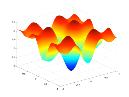
Figure 1: The function $f$

The input vector $\mathbf{X}$ is supposed to have a uniform distribution on $E$. The threshold is set to $\rho=0.01$ which corresponds to the probability
$\mathbb{P}_{\mathbf{X}}\left(f(\mathbf{X})<\rho\right)=4.72\cdot 10^{-4}$. This probability was computed thanks to a massive Monte Carlo integration.
It is assumed that no more than $N=100$ calls to $f$ are allowed. For the Bayesian strategy, all of the $N=100$ available calls to $f$ are used to build the metamodel, while for the MBIS strategy (using notations of Section 3) $n=50$ and $m=50$ are set. The two strategies are compared with different design sampling methods. Three design sampling methods are used: an LHS-maximin method (Morris and Mitchell,, 1995) which is non sequential and space filling and two sequential methods. The sequential sampling methods are based on a first LHS-maximin design including $80\%$ of the points and the last $20\%$ are added sequentially according to the criterion tIMSE (targeted Integrated Mean Square Error) proposed by Picheny et al., (2010) for one method and according to the criterion J SUR (Stepwise Uncertainty Reduction) proposed by Bect et al., (2011) for the other method. These sequential methods are based on a trade-off between reduction of uncertainty in the knowledge of $f$ and the exploration of the space around the critical set $R_{\rho}$. All Kriging metamodels are built with an intercept as the regression function and a Gaussian correlation function is chosen as the correlation function of the Gaussian process $\zeta$ i.e. $\forall\mathbf{x}\in E$, $h(\mathbf{x})=1$ and $\forall\mathbf{x},\mathbf{x}^{\prime}\in E$, $K(\mathbf{x},\mathbf{x})=\exp\left(-\theta\|\mathbf{x}-\mathbf{x}^{\prime}\|^{2}\right)$ are set for the model given by equation (2.1). For the Bayesian strategy, a thousand realizations of $\Pi_{\rho}^{D_{N}}$ are computed from which the credible bound is obtained. The discretization is done on a grid with $100$ points and to prevent ill-conditioned covariance matrices, if a point of the grid is too close to a point of the design $D_{N}$ it is replaced with a point in $E$ far enough from the points of the design and the points of the grid. The numerical integration to compute the realization of $\Pi_{\rho}^{D_{N}}$ from the realization of the process is done with a $10^{5}$-sample. In the MBIS strategy, the probability $\mathbb{P}_{\mathbf{X}}(\hat{R}_{\rho,\kappa})$ (and also the bound on the bias, given in Proposition 3.2) was computed by a Monte Carlo integration on a $10^{7}$-sample and $\kappa=3$ has been set.

There are sources of variability on the estimators and the bounds due to the design sampling methods. Indeed, the designs are computed to be maximin by using a finite number of iterations of a simulated annealing algorithm. Moreover, there exist symmetries within the class of maximin designs. In the sequential method, the point to be added is sought through a stochastic algorithm. Concerning the importance sampling strategy, the sampling which gives $\mathbf{Z}_{1:m}$ induces variability. In order to test the sensitivity to these sources of variability, each of the two strategies for each of the three design sampling methods is repeated one hundred times.

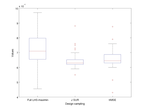
Figure 2: Bayesian $98\%$ credible bound for $\pi_{\rho}$

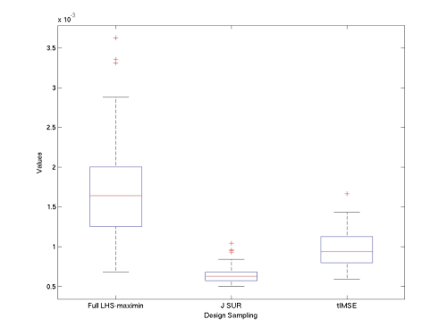
Figure 3: MBIS $98\%$ stochastic bounds of $\pi_{\rho}$

	Full LHS-maximin	J SUR	tIMSE
Minimum	$4.55$	$5.50$	$4.30$
$1^{\text{st}}$ quartile	$6.55$	$6.20$	$6.30$
Mean	$7.78$	$7.58$	$52.2$
Median	$7.10$	$6.30$	$6.45$
$3^{\text{rd}}$ quartile	$7.97$	$6.52$	$6.87$
Maximum	$35.3$	$55.4$	$3027$

Table 1: Bayesian $98\%$ credible bound of $\pi_{\rho}$ multiplied by $10^{4}$

	Full LHS-maximin	J SUR	tIMSE
Minimum	$6.82$	$4.98$	$5.88$
$1^{\text{st}}$ quartile	$12.58$	$5.71$	$8.00$
Mean	$16.8$	$6.43$	$9.67$
Median	$16.4$	$6.28$	$9.39$
$3^{\text{rd}}$ quartile	$20.1$	$6.81$	$11.3$
Maximum	$36.3$	$10.4$	$16.7$

Table 2: IS $98\%$ stochastic bounds of $\pi_{\rho}$ multiplied by $10^{4}$

Figure 2 and Table 1 display the results for $98\%$ credible bounds obtained by the Bayesian strategy and Figure 3 and Table 2 display the results for $98\%$ stochastic bounds obtained by the MBIS strategy. The results are provided according to the design sampling method. For the MBIS stochastic bounds, $\alpha=1\%$ and $\beta=1\%$ have been set using the notations of Proposition 3.3. If a crude Monte Carlo scheme as presented in Section 1 is used here with only $N=100$ calls, the estimator is equal to $0$ with probability greater than $0.95$ and in this case, the upper confidence bound is $0.038$ at level $98\%$. The two strategies bring much sharper bounds on the probability of the rare event. The sequential design sampling method with J SUR criterion leads to the better bounds whatever the strategy. The MBIS strategy manages to reach the same sharp bounds as the ones provided by the Bayesian strategy in the case where the design is obtained thanks to the J SUR criterion. The Bayesian strategy is less sensitive to the choice in the design sampling method. However, the Bayesian method suffers from the fact that the quantiles are estimated thanks to conditional simulations of the Gaussian process which rely on a discretization of the space. Hence, it leads to an approximation in results and stability concern as is noticed in the results (see the maximum credible bound obtained with the tIMSE sampling criterion). Furthermore, a limited number of iterations is achievable since the simulations are quite burdensome.

The bound provided by Markov inequality (2.6) is not interesting in this example since it cannot be less than 0.01. Chebychev inequality has not been used since we were not able to determine the posterior variance in a reasonable time.

As the strategies depend on the Kriging model hypothesis (2.1), a leave-one-out cross validation as proposed by Jones et al., (1998) can be performed to check whether this hypothesis is sensible. It consists of building $n$ metamodels with posterior mean and variance denoted respectively by $m_{D_{n}^{-i}}$ and $\sigma^{2}_{D_{n}^{-i}}$, from designs

$$D_{n}^{-i}=\{\mathbf{x}_{1},\ldots,\mathbf{x}_{i-1},\mathbf{x}_{i+1},\ldots,\mathbf{x}_{n}\}\,,$$

where $i=1,\ldots,n$.
Then, the values

$$\frac{|f(\mathbf{x}_{i})-m_{D_{n}^{-i}}(\mathbf{x}_{i})|}{\sigma^{2}_{D_{n}^{-i}}(\mathbf{x}_{i})}\,,$$ (4.1)

are computed. If something like $99.7\%$ of them lie in the interval $[-3,3]$, the Kriging hypothesis is not rejected. In our toy example, in all of the tests which were done, all these values are in $[-2,2]$.

4.2 A real case study: release envelope clearance

4.2.1 Context

When releasing an airborne load, a critical issue is the risk that its trajectory could collide with the aircraft. The behavior of such a load after release depends on many variables. Some are under the control of the crew: mach, altitude, load factor, etc. We call them controlled variables and denote their variation domain as $C$. The others are uncontrolled variables: let $E$ be the set of their possible values. The release envelope clearance problem consists of exploring the set $C$ to find a subset where the release is safe, whatever the uncontrolled variables are. To investigate this problem, we can use a simulator which computes the trajectory of the carriage when the values of all the variables are given. Moreover, for $\mathbf{x}_{C}\in C$ and $\mathbf{x}\in E$, besides the trajectory $\tau(\mathbf{x}_{C},\mathbf{x})$, the program delivers a danger score $f(\mathbf{x}_{C},\mathbf{x})$ to be interpreted as an “algebraic distance”: a negative value characterizes a collision trajectory.
To assess the safety of release at a given point of $C$, we suppose that the values of the uncontrolled variables are realizations of a random variable $\mathbf{X}\in E$ that can be simulated. Therefore, for a given value $\mathbf{x}_{C}\in C$, and $\rho\geq 0$ the $\rho$-collision risk is the probability

$$\pi_{\rho}(\mathbf{x}_{C})=\mathbb{P}(f(\mathbf{x}_{C},\mathbf{X})<\rho)\,.$$

We do not aim at estimating this risk accurately.
We would rather classify the points into three categories: according to the position of $0$-risk $\pi_{0}(\mathbf{x}_{C})$ with respect to the two markers $10^{-5}$ and $10^{-2}$, $\mathbf{x}_{C}$ is said to be

1. totally safe if $\pi_{0}(\mathbf{x}_{C})\leq 10^{-5}$,

2. relatively safe if $10^{-5}<\pi_{0}(\mathbf{x}_{C})<10^{-2}$,

3. unsafe if $\pi_{0}(\mathbf{x}_{C})\geq 10^{-2}$.

In this example, there are $5$ controlled and $26$ uncontrolled variables, so that $C\subset\mathbb{R}^{5},E\subset\mathbb{R}^{26}$. From budgetary point of view, experts consider that a set of about $400$ representative points of $C$ is enough to cover the domain $C$ consistently. On the other hand, the computation of $800,000$ trajectories takes about 4 days which is considered reasonable. On the basis of these indications, the maximum amount of available calls to the simulator is $N=2000$ per point.

4.2.2 Bounding strategy

As the dimension of the set of uncontrolled variables $E$ is high, the credible bounds obtained with the Bayesian strategy are impossible to get. The stochastic bounds provided by the MBIS strategy are still available. Unfortunately, a sequential sampling method for the design of experiments is not achievable since the simulator is too expensive if only one point is evaluated per call. Indeed, a fixed part of the cost of a call does not depend on the number of points for which the code is run. Although the MBIS strategy with an LHS-maximin sampling method is not optimal, it is still efficient.

We propose this two-step bounding strategy which can be applied for each point of the set of representative points (in the set $C$). Each step uses half of the calls budget: $m=n=\frac{N}{2}=1000$. Let $\mathbf{x}_{C}\in C$ be the current point of interest that we suppose fixed. For any $\mathbf{x}\in E$, $f(\mathbf{x})=f(\mathbf{x}_{C},\mathbf{x})$ is set. It then corresponds to the notation introduced in the first part of the paper.

1. At the first stage, a Gaussian process is built as explained in (2), on the basis of evaluations $f(\mathbf{x}_{1}),\cdots,f(\mathbf{x}_{n})\in\mathbb{R}^{n}$ of $f$ on $D_{n}=\{\mathbf{x}_{1},\cdots,\mathbf{x}_{n}\}$. We know that $\pi_{\rho}$ is a realization of the random variable $\Pi_{\rho}^{D_{n}}$ whose mean

   $$\mathbb{E}(\Pi_{\rho}^{D_{n}})=\mathbb{E}\left(\Phi\left(\frac{\rho-m_{D_{n}}(\mathbf{X})}{\sqrt{K_{D_{n}}(\mathbf{X},\mathbf{X})}}\right)\right)\,,$$

   can be computed accurately.
   As stated by (2.6), applying Markov inequality gives, for any $\alpha\in]0;1[$,

   $$\mathbb{P}\left(\Pi_{\rho}^{D_{n}}\leq\frac{\mathbb{E}(\Pi_{\rho}^{D_{n}})}{\alpha}\right)\geq 1-\alpha\,.$$

   According to the value of $\mathbb{E}(\Pi_{\rho}^{D_{n}})$ we then take the following decisions:

   • if $\mathbb{E}(\Pi_{\rho}^{D_{n}})\leq\frac{1}{2}10^{-10}$ which leads by (2.6) to $\mathbb{P}\left(\Pi_{\rho}^{D_{n}}\leq\frac{10^{-5}}{2}\right)\geq 1-\frac{10^{-5}}{2}$, we qualify the current point $\mathbf{x}_{C}\in C$ as totally safe,

   • if $\mathbb{E}(\Pi_{\rho}^{D_{n}})\geq 10^{-2}$, we conservatively classify $\mathbf{x}_{C}$ as unsafe,

   • if $\frac{1}{2}10^{-10}<\mathbb{E}(\Pi_{\rho}^{D_{n}})<10^{-2}$ we use a second stage procedure to refine the risk assessment.

2. A million-sample $\mathbf{x}_{1},\cdots,\mathbf{x}_{M}$ of $\mathbf{X}$ is drawn from which we tune $\kappa$ in such a way that $m=1000$ of these million elements of $E$ are in $\hat{R}_{\rho,\kappa}$. The resulting points $\mathbf{z}_{1},\cdots,\mathbf{z}_{m}$ are an $m$-sample $\mathbf{z}_{1:m}$ of realizations of the random variable $\mathbf{Z}$ which follows the importance distribution,
   

   $$\mathbb{P}_{\mathbf{Z}}:A\mapsto\mathbb{P}_{\mathbf{X}}(A|\hat{R}_{\rho,\kappa})\,.$$

   By using $m$ calls to the simulator, $\Gamma(f,\mathbf{z}_{1:m},\rho)$ is computed. Drawn from Proposition 3.3 with setting $\alpha=\beta$, we obtain the bound

   $$b(\Gamma(f,\mathbf{z}_{1:m},\rho),m,\alpha)\mathbb{P}_{\mathbf{X}}(\hat{R}_{\rho,\kappa})+\frac{c(\kappa)}{\alpha}\,,$$

   which is a decreasing function of $\alpha$.
   Let us define $\alpha_{0}=\min\{\alpha:b(\Gamma(f,\mathbf{z}_{1:m},\rho),m,\alpha)\mathbb{P}_{\mathbf{X}}(\hat{R}_{\rho,\kappa})+\frac{c(\kappa)}{\alpha}\leq 2\alpha\}$. For such an $\alpha_{0}$, Proposition 3.3 states:

   $$\mathbb{P}\left(\Pi_{\rho}^{D_{n}}\leq b(\Gamma(F^{D_{n}},\mathbf{Z}_{1:m},\rho),m,\alpha_{0})\mathbb{P}_{\mathbf{X}}(\hat{R}_{\rho})+\frac{c(\kappa)}{\alpha_{0}}\right)\geq 1-2\alpha_{0}\,,$$

   which provides $2\alpha_{0}$ as a $1-2\alpha_{0}$ confidence upper bound on $\pi_{\rho}$.

4.2.3 Experiments

Three points of $C$ have been experienced. Of these cases the first one is known to be a null $0$-risk point, while the third one is very unsafe and the second one is in-between. For benchmarking purposes, besides the simulator calls budget required for the estimation process described in 4.2.2, a $10,000$ sample of realizations of $f(\mathbf{x}_{E},\mathbf{X})$ has been computed for each of the three examples. For each case, we began by estimating a Gaussian process on the basis of $f$-values computed on the points of a $1000$-point design $D_{n}=\{\mathbf{x}_{1},\cdots,\mathbf{x}_{n}\}$. This design was obtained by LHS-maximin sampling. Figures 4, 5 and 6 show the predictive performance of the processes when applied to the benchmark points. These points, which appear in red, are sorted according to their process mean values while the blue curves mark the predicted 3 standard deviation positions around the means. As appears rather clearly, the dispersion of the real values is underestimated by the model: they overflow the blue zone with a frequency ($\sim 5\%$) higher than expected ($0.27\%$). The worst case is the first one, for which large deviations appear for benchmark points with low values of $f$.

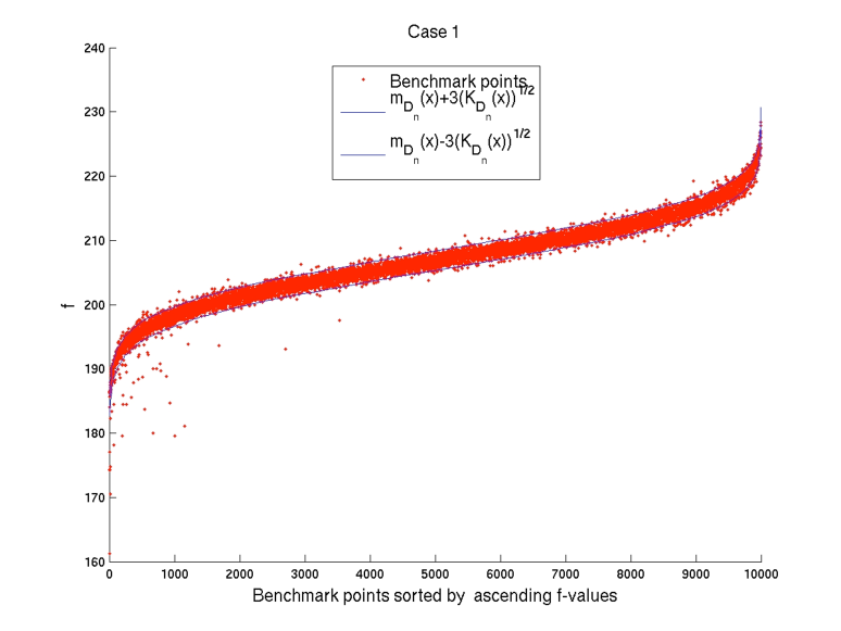
Figure 4: Prediction performance case 1

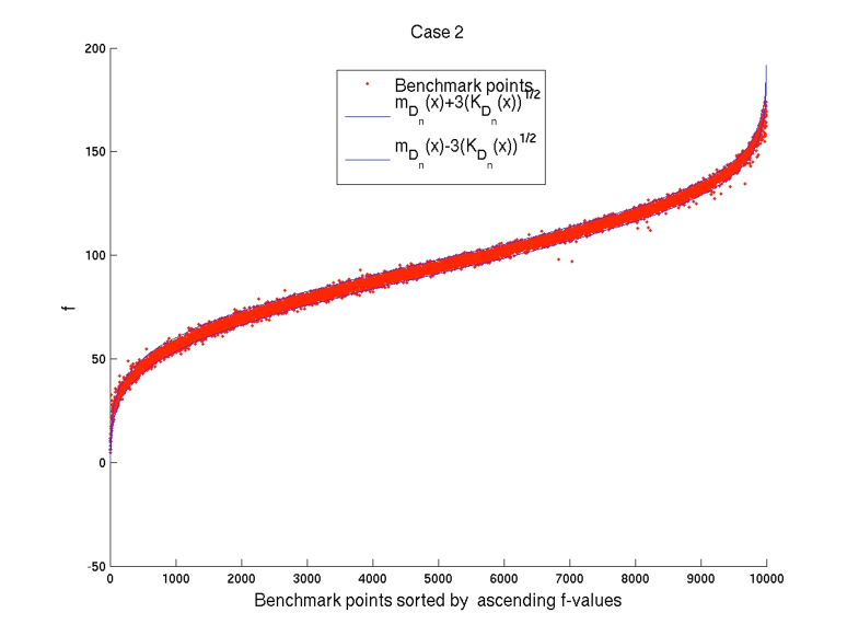
Figure 5: Prediction performance case 2

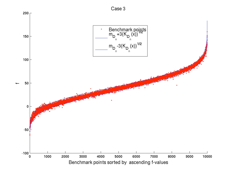
Figure 6: Prediction performance case 3

In order to obtain bounds from (2.6), we then computed $\mathbb{E}(\Pi_{0}^{D_{n}})$ using (2.4):

• In the first case, the massive Monte Carlo procedure leads to a numerically null evaluation of $\mathbb{E}(\Pi_{0}^{D_{n}})$ and, as a consequence, to the classification of the related $C$ point as totally safe.

• In the second example, $\mathbb{E}(\Pi_{0}^{D_{n}})$ being evaluated at $1.68\ 10^{-4}$, we need to proceed to the second step of the bounding strategy to refine the collision probability estimation. The obtained confidence upper bound is $1.2\ 10^{-5}$ at confidence level $1-1.2\ 10^{-5}$. The benchmark data do not show collision case: a $90\%$ confidence upper bound is $2.3\ 10^{-4}$.

• $\mathbb{E}(\Pi_{0}^{D_{n}})=0.103$ in case 3 which is consistent with the $90\%$ confidence interval $[0.0999;0.1101]$, obtained on benchmark data.

5 Discussion

In this paper, we have especially focused on bounding the probability of a rare event. From our point of view, it seems much more reliable to assess that the probability of a feared event (failure of a system, natural disaster, etc.) not exceeding a given level with high probability than to estimate the probability of this event happening. Using Kriging metamodels to cope with the expensive black box model induces a random interpretation of the probability to be estimated. Two strategies were studied in that context including our MBIS strategy. On a toy example, the efficiency of the two strategies was shown and it was highlighted that a sequential design sampling, when possible, is preferable. Concerning the importance sampling strategy, further investigations could be about proposing an optimal splitting of the calls to the code used for the metamodel or for the importance sampling. Other concerns could be about tuning $\kappa$ to construct the set $\hat{R}_{\rho,\kappa}$.

We have dealt with a cross-validation method to assess the Kriging hypothesis. However, in the case where the cross-validation leads one to reconsider this hypothesis, a solution is to extend the confidence interval on the prediction by tuning by hand the parameter $\sigma^{2}$ in equation (2.1). In Bayesian words, it can be called using a less informative prior distribution on $f$.

We have not managed to compute the posterior variance (2.5) by using a massive Monte Carlo integration in our examples since it is very small. However, other rare event methods can be investigated since the variance no longer depends on $f$.

References

- Bect et al., (2011) Bect, J., Ginsbourger, D., Li, L., Picheny, V., and Vazquez, E. (2011). Sequential design of computer experiments for the estimation of a probability of failure. Statistics and Computing. to appear.
- Bingham et al., (2006) Bingham, D., Hengartner, N., Higdon, D., and Kenny, Q. Y. (2006). Variable Selection for Gaussian Process Models in Computer Experiments. Technometrics, 48(4):478–490.
- Cannamela et al., (2008) Cannamela, C., Garnier, J., and Iooss, B. (2008). Controlled stratification for quantile estimation. The Annals of Applied Statistics, 2(4):1554–1580.
- (4) Cérou, F. and Guyader, A. (2007a). Adaptive multilevel splitting for rare event analysis. Stochastic Analysis and Applications, 25(2):417–443.
- (5) Cérou, F. and Guyader, A. (2007b). Adaptive particle techniques and rare event estimation. In Conference Oxford sur les méthodes de Monte Carlo séquentielles, volume 19 of ESAIM Proc., pages 65–72. EDP Sci., Les Ulis.
- Del Moral and Garnier, (2005) Del Moral, P. and Garnier, J. (2005). Genealogical particle analysis of rare events. The Annals of Applied Probability, 15(4):2496–2534.
- Dette and Pepelyshev, (2010) Dette, H. and Pepelyshev, A. (2010). Generalized Latin Hypercube Design for Computer Experiments. Technometrics, 52(4):421–429.
- Fang et al., (2006) Fang, K.-T., Li, R., and Sudjianto, A. (2006). Design and Modeling for Computer Experiments. Computer Science and Data Analysis. Chapman & Hall/CRC.
- Heidelberg, (1995) Heidelberg, P. (1995). Fast simulation of rare events in queuing and reliability models. ACM Transactions on Modeling and Computer Simulation, 5:43–85.
- Jones et al., (1998) Jones, D. R., Schonlau, M., and Welch, W. J. (1998). Efficient Global Optimization of Expensive Black-Box Functions. Journal of Global Optimization, 13(4):455–492.
- Joseph, (2006) Joseph, V. R. (2006). Limit Kriging. Technometrics, 48(4):458–466.
- Koehler and Owen, (1996) Koehler, J. and Owen, A. (1996). Computer experiments. In Design and analysis of experiments, volume 13 of Handbook of Statistics, pages 261–308. North Holland, Amsterdam.
- L’Ecuyer et al., (2007) L’Ecuyer, P., Demers, V., and Tuffin, B. (2007). Rare events, splitting, and quasi-Monte Carlo. ACM Trans. Model. Comput. Simul., 17(2).
- Li and Sudjianto, (2005) Li, R. and Sudjianto, A. (2005). Analysis of Computer Experiments using Penalized Likelihood in Gaussian Kriging Models. Technometrics, 47(2):111–120.
- Mease and Bingham, (2006) Mease, D. and Bingham, D. (2006). Latin Hyperrectangle Sampling for Computer Experiments. Technometrics, 48(4):467–477.
- Morris and Mitchell, (1995) Morris, M. and Mitchell, T. (1995). Exploratory designs for computer experiments. Journal of Statistical Planning and Inference, 43:381–402.
- Munoz Zuniga et al., (2010) Munoz Zuniga, M., Garnier, J., Remy, E., and de Rocquigny, E. (2010). Adaptative directional stratification for controlled estimation of the probability of a rare event. Technical report.
- Oakley, (2004) Oakley, J. (2004). Estimating percentiles of uncertain computer code outputs. Applied Statistics, 53:83–93.
- Picheny et al., (2010) Picheny, V., Ginsbourger, D., Roustant, O., and Haftka, R. (2010). Adaptive designs of experiments for accurate approximation of a target region. Journal of Mechanical Design, 132(7).
- Santner et al., (2003) Santner, T., Williams, B., and Notz, W. (2003). The Design and Analysis of Computer Experiments. Springer-Verlag.
- Shahabuddin, (1995) Shahabuddin, P. (1995). Rare event simulation in stochastic models. In WSC’95: Proceedings of the 27th conference on Winter simulation.
- Vazquez and Bect, (2009) Vazquez, E. and Bect, J. (2009). A sequential Bayesian algorithm to estimate a probability of failure. In 15th IFAC SYmposium on System IDentification (SYSID 2009).
- Welch et al., (1992) Welch, W. J., Buck, R. J., Sack, J., Wynn, H. P., Mitchell, T. J., and Morris, M. D. (1992). Screening, Predicting, and Computer Experiments. Technometrics, 34(1):15–25.