Exotic leaky wave radiation from anisotropic epsilon near zero metamaterials

Abstract

We investigate the emission of electromagnetic waves from biaxial subwavelength metamaterials. For tunable anisotropic structures that exhibit a vanishing dielectric response along a given axis, we find remarkable variation in the launch angles of energy associated with the emission of leaky wave radiation. We write closed form expressions for the energy transport velocity and corresponding radiation angle $\varphi$, defining the cone of radiation emission, both as a functions of frequency, and material and geometrical parameters. Full wave simulations exemplify the broad range of directivity that can be achieved in these structures.

Metamaterials are composite structures engineered with subwavelength components, and with the purpose of manipulating and directing electromagnetic (EM) radiation. Recently many practical applications have emerged, and structures fabricated related to cloaking, metamaterial perfect absorbers liu2 , and chirality zhang2 ; menzel . For metamaterials, the desired EM response to the incident electric (${\bm{E}}$) and magnetic (${\bm{H}}$) fields, typically involves tuning the permittivity, $\epsilon$, and permeability, $\mu$ in rather extraordinary ways. This includes double negative index media (negative real parts of both $\epsilon$ and $\mu$), single negative index media (negative real part of $\epsilon$ or $\mu$), matched impedance zero index media zio ; cuong (real part of $\epsilon$ and $\mu$ is near zero), and epsilon near zero (ENZ) media (real part of $\epsilon$ is near zero). Scenarios involving ENZ media in particular have gained prominence lately as useful components to radiative systems over a broad range of the EM spectrum enoch ; eng ; alu .

In conjunction with ENZ developments, there have also been advances in infrared metamaterials, where thermal emitters laroche , optical switches shen , and negative index metamaterials zhang ; zhang2 have been fabricated. Due to the broad possibilities in sensing technologies, this EM band is of considerable importance. Smaller scale metamaterial devices can also offer more complex and interesting scenarios, including tunable devices souk , filters alek , and nanoantennas liu . For larger scale ENZ metamaterials, high directivity of an incident beam has been demonstrated enoch . This can be scaled down and extended to composites containing an array of nanowires, yielding a birefringent response with only one direction possessing ENZ properties alek . A metamaterial grating can be designed to also have properties akin to ENZ media mocella .

Often times, the structure being modeled is assumed isotropic. Although this offers simplifications, anisotropy is an inextricable feature of metamaterials that plays a crucial role in their EM response. For instance, at optical and infrared frequencies, incorporating anisotropy into a thin planar (nonmagnetic) waveguide can result in behavior indicative of double negative index media pod . Anisotropic metamaterial structures can now be created that contain elements that possess extreme electric and magnetic responses to an incident beam. The inclusion of naturally anisotropic materials that are also frequency dispersive (e.g., liquid crystals), allows additional control in beam direction. It has also been shown that metamaterial structures requiring anisotropic permittivity and permeability can be created using tapered waveguides smol . By assimilating anisotropic metamaterial leaky wave structures within conventional radiative systems, the possibility exists to further control the emission characteristics.

Prompted by submicron experimental developments, and potential beam manipulation involving metamaterials with vanishing dielectric response, we investigate a planar anisotropic system with an ENZ response at near-ir frequencies along a given (longitudinal) direction. By “freezing” the phase in the longitudinal direction and tuning the electric and magnetic responses in the transverse directions, we will demonstrate the ability to achieve remarkable emission control and directivity. When excited by a source, the direction of energy flow can be due to the propagation of localized surface waves. There can also exist leaky waves, whereby the energy radiatively “leaks” from the structure while attenuating longitudinally. Indeed, there can be a complex interplay between the different type of allowed modes whether radiated or guided, or some other mechanism involving material absorption. Through a judicious choice of parameters, the admitted modes for the metamaterial can result in radiation launched within a narrow cone spanned by the outflow of energy flux.

Some of the earliest works involving conventional leaky wave systems reported narrow beamwidth antennas with prescribed radiation angles tamir , and forward/backward leaky wave propagation in planar multilayered structures tamir2 . In the microwave regime, photonic crystals colak ; micco ; laroche and transmission lines can also can serve as leaky wave antennas lim . More recently, a leaky wave metamaterial antenna exhibited broad side scanning at a single frequency lim . The leaky wave characteristics have also been studied for grounded single and double negative metamaterial slabs bacc . Directive emission in the microwave regime was demonstrated for magnetic metamaterials in which one of the components of $\bm{\mu}$ is small yuan . Nonmagnetic slabs can also yield varied beam directivity slab2 .

To begin our investigation, a harmonic time dependence $\exp(-i\omega t)$ for the TM fields is assumed. The planar structure contains a central biaxial anisotropic metamaterial of width $2d$ sandwiched between the bulk superstrate and substrate, each of which can in general be anisotropic. The material in each region is assumed linear with a biaxial permittivity tensor, $\bm{\epsilon}_{i}=\epsilon_{i}^{xx}\hat{\bf x}\hat{\bf x}+\epsilon_{i}^{yy}\hat{\bf y}\hat{\bf y}+\epsilon_{i}^{zz}\hat{\bf z}\hat{\bf z}$. Similarly, the biaxial magnetic response is represented via ${\bm{\mu}}_{i}=\mu_{i}^{xx}\hat{\bf x}\hat{\bf x}+\mu_{i}^{yy}\hat{\bf y}\hat{\bf y}+\mu_{i}^{zz}\hat{\bf z}\hat{\bf z}$. The translational invariance in the $y$ and $z$ directions allows the magnetic field in the $i$th layer, ${\bf H}_{i}$, to be written ${\bf H}_{i}=\hat{\bm{y}}h_{i}^{y}(x)e^{i(\gamma z-\omega t)}$, and the electric field as ${\bf E}_{i}=[\hat{\bm{x}}e_{i}^{x}(x)+\hat{\bm{z}}e_{i}^{z}(x)]e^{i(\gamma z-\omega t)}$. Here, $\gamma\equiv\beta+i\alpha$ is the complex longitudinal propagation constant. We focus on wave propagation occurring in the positive $x$ direction, and nonnegative $\beta$ and $\alpha$. Upon matching the tangential $\bm{E}$ and $\bm{H}$ fields at the boundary, we arrive at the general dispersion equation that governs the allowed modes for this structure,

$$\epsilon^{zz}_{2}k_{\perp,2} (\epsilon^{zz}_{3}k_{\perp,1}+\epsilon^{zz}_{1}k_{\perp,3})+$$ (1)

$$[(\epsilon^{zz}_{2})^{2}k_{\perp,1}k_{\perp,3}-\epsilon^{zz}_{1}\epsilon^{zz}_{3}k^{2}_{\perp,2}]\tan(2dk_{\perp,2})=0,$$

where the transverse wavevector in the superstrate (referred to as region 1), $k_{\perp,1}$, is,

$$k_{\perp,1}=\pm\sqrt{\epsilon_{1}^{zz}/\epsilon_{1}^{xx}(\beta^{2}-\alpha^{2})-k_{0}^{2}\mu_{1}^{yy}\epsilon_{1}^{zz}+2i\alpha\beta\epsilon_{1}^{zz}/\epsilon_{1}^{xx}}.$$ (2)

For the metamaterial region (region 2), we write $k_{\perp,2}=\pm\sqrt{k_{0}^{2}\mu_{2}^{yy}\epsilon_{2}^{zz}-\gamma^{2}\epsilon_{2}^{zz}/\epsilon_{2}^{xx}}$, and for the substrate (region 3), $k_{\perp,3}=\pm\sqrt{\gamma^{2}\epsilon_{3}^{zz}/\epsilon_{3}^{xx}-k_{0}^{2}\mu_{3}^{yy}\epsilon_{3}^{zz}}$. The choice of sign in regions 1 and 3 plays an important role in the determination of the physical nature of the type of mode solution that will arise. The two roots associated with $k_{\perp,2}$, results in the same solutions to Eq. (1). The dispersion (Eq. (1)) is also obtained from the poles of the reflection coefficient for a plane wave incident from above on the structure. The transverse components of the ${\bm{E}}$ field in region 1 are, $e_{1}^{z}=-ik_{\perp,1}/(k_{0}\epsilon^{zz}_{1})H_{1}e^{-k_{\perp,1}(x-d)}$, $e_{1}^{x}=\gamma/(k_{0}\epsilon^{xx}_{1})h_{1}^{y}$, and $h_{1}^{y}=H_{1}e^{-k_{\perp,1}(x-d)}$, where $H_{1}$ is a constant coefficient.

Next, to disentangle the evanescent and leaky wave fields, we separate the wavevector $k_{\perp,1}$ into its real and imaginary parts: $k_{\perp,1}=\pm(q^{-}+iq^{+})$, with $q^{+}$ and $q^{-}$ real. The $k_{\perp,1}$, $q^{-}$, and $q^{+}$ are in general related, depending on $\operatorname{sgn}(\epsilon_{1}^{zz}\alpha\beta/\epsilon_{1}^{xx})$. For upward wave propagation ($+x$ direction), clearly we have $q^{+}q^{-}\geq 0$. It is also apparent that the parameter $q^{-}$ represents the inverse length scale of wave increase along the transverse $x$-direction. We are mainly concerned with the $k_{\perp,1}$ that correspond to exponential wave increase in the transverse direction while decaying in $z$, a hallmark of leaky waves. Although leaky wave modes are not localized, they can be excited by a point or line source which gives rise to limited regions of space of EM wave amplitude increase before eventually decaying. When explicitly decomposing $k_{\perp,1}$ into its real and imaginary parts, there is an intricate interdependence among $\gamma$, $\bm{\epsilon}_{i}$, and $\bm{\mu}_{i}$ (for $\alpha\neq 0$): $q^{\pm}=1/\sqrt{2}(\sqrt{{\cal A}^{2}+{\cal B}^{2}}\mp{\cal A})^{1/2}$, where ${\cal A}=\epsilon_{1}^{zz}/\epsilon_{1}^{xx}(\beta^{2}-\alpha^{2})-k_{0}^{2}\mu_{1}^{yy}\epsilon_{1}^{zz}$, and ${\cal B}=2\alpha\beta\epsilon_{1}^{zz}/\epsilon_{1}^{xx}$. We will see below that $q^{+}$ is the root of interest in determining leaky wave emission for our structure. At this point the surrounding media can have frequency dispersion in $\bm{\epsilon}_{i}$, and $\bm{\mu}_{i}$, while the anisotropic metamaterial region can be dispersive and absorptive.

We are ultimately interested in anisotropic metamaterials with an ENZ response along the axial direction ($z$-axis). In the limit of vanishing $\epsilon_{2}^{zz}$, and perfectly conducting ground plane, Eq. (1) can be solved analytically for the complex propagation constant, $\gamma$. The result is

$$\gamma^{\pm}=\dfrac{1}{\sqrt{2}}\dfrac{\sqrt{(\epsilon_{2}^{xx})^{2}+8(k_{0}d)^{2}\epsilon_{1}^{xx}\epsilon_{1}^{zz}\epsilon_{2}^{xx}\mu_{2}^{yy}\pm\left|\epsilon_{2}^{xx}\right|\sqrt{(\epsilon_{2}^{xx})^{2}+(4k_{0}d)^{2}\epsilon_{1}^{zz}\epsilon_{1}^{xx}(\mu_{2}^{yy}\epsilon_{2}^{xx}-\mu_{1}^{yy}\epsilon_{1}^{xx})}}}{2k_{0}d\sqrt{\epsilon_{1}^{xx}\epsilon_{1}^{zz}}}.$$ (3)

The two possible roots correspond to distinct dispersion branches (seen below). There are, in all, four solutions, $\gamma^{\pm}$, and $-\gamma^{\pm}$. The geometrical and material dependence contained in Eq. (3), determines the entire spectrum of the leaky radiation fields that may exist in our system.

There are numerous quantities one can study in order to effectively characterize leaky wave emission. One physically meaningful quantity is the energy transport velocity, ${\bm{v}}_{T}$, which is the velocity at which EM energy is transported through a medium loudon ; ruppin . It is intuitively expressed as the ratio of the time-averaged Poynting vector, ${\bm{S}}_{\rm avg}$, to the energy density, $U$: ${\bm{v}}_{T}\equiv{\bm{S}}_{\rm avg}/U$. Properly accounting for frequency dispersion that may be present, we can thus write the energy velocity for EM radiation emitted above the structure,

$${\bm{v}}_{T}=\dfrac{c/(8\pi){\rm Re}[{\bm{E}}_{1}\times{\bm{H}}_{1}^{*}]}{1/(16\pi)\Bigl{[}{\bm{E}}_{1}^{\dagger}\cdot\dfrac{d(\omega{\bm{\epsilon}}_{1})}{d\omega}{\bm{E}}_{1}+{\bm{H}}_{1}^{\dagger}\cdot\dfrac{d(\omega{\bm{\mu}}_{1})}{d\omega}{\bm{H}}_{1}\Bigr{]}},$$ (4)

where the conventional definition shitz of $U$ has been extended to include anisotropy. Inserting the calculated EM fields, we get the compact expression (assuming no dispersion in the superstrate),

$${\bm{v}}_{T}=\omega\dfrac{\bigl{(}\epsilon_{1}^{xx}q^{+}\hat{\bm{x}}+\epsilon_{1}^{zz}\beta\hat{\bm{z}}\bigr{)}}{\epsilon_{1}^{zz}\beta^{2}+\epsilon_{1}^{xx}(q^{+})^{2}}.$$ (5)

The corresponding direction of energy outflow is straightforwardly extracted from the vector directionality in Eq. (5),

$$\varphi=\tan^{-1}\bigl{(}\dfrac{\epsilon_{1}^{xx}q^{+}}{\epsilon_{1}^{zz}\beta}\bigr{)},$$ (6)

which holds in the case of loss and frequency dispersion in the metamaterial. It is evident that Eq. (6) satisfies $\varphi\rightarrow 0$ as $\alpha\rightarrow 0$, corresponding to the disappearance of the radiation cone and possible emergence of guided waves. In this limit, ${\bm{v}}_{T}=\hat{\bm{z}}\omega/\beta$, which corresponds to the expected phase velocity, or velocity at which plane wavefronts travel along the $z$-direction. There is also angular symmetry, where $\varphi(\epsilon_{2}^{xx})\rightarrow\varphi(-\epsilon_{2}^{xx})$, when $\mu_{2}^{yy}\rightarrow-\mu_{2}^{yy}$. For high refractive index media ($\epsilon_{2}^{xx}$ or $\mu_{2}^{yy}$ $\rightarrow\infty$), we moreover recover the expected result that $\varphi$ tends toward broadside ($\varphi=0$).

Leaky wave emission from an anisotropic metamaterial in vacuum

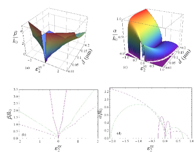
Figure 1: (Color online). The real ($\beta$) and imaginary ($\alpha$) parts of the complex propagation constant $\gamma^{+}$, normalized by the vacuum wavevector $k_{0}$ at $f=280$ THz ($\mu_{2}^{yy}=1$). The figures (a) and (c) are 3D global views depicting $\alpha$ and $\beta$ as functions of $\epsilon_{2}^{xx}$ and the thickness parameter $d$. Figures (b) and (d) represent the normalized $\beta$ and $\alpha$, respectively, as functions of $\epsilon_{2}^{xx}$ and for $d=0.01$ µm (solid curve), $d=0.05$ µm (dotted curve), and $d=0.1$ µm (dashed curve).

is characterized in Figs. 1 (a) and (c), where 3-D views of the normalized $\beta$ (${\rm Re}[\gamma^{+}]$), and $\alpha$ (${\rm Im}[\gamma^{+}]$), are shown as functions of the transverse dielectric response, $\epsilon_{2}^{xx}$, and thickness parameter, $d$ (the width = $2d$). In Fig. 1 (b) and (d), 2D slices depict the normalized $\beta$ and $\alpha$ as functions of $\epsilon_{2}^{xx}$. Only the positive root, $\gamma^{+}$, is shown, corresponding to the leaky wave case of interest, with $\alpha\geq 0$. The slight kinks in the curves (see Fig. 1(b)) are at points where the $\gamma^{-}$ solutions would emerge (for $\alpha<0$). Both panels on the left clearly demonstrate how $\beta$ rises considerably with increasing $|\epsilon_{2}^{xx}|$. For subwavelength widths ($k_{0}d\ll 1$), and to lowest order, the propagation constant varies linearly in $\epsilon_{2}^{xx}$, as $\beta/k_{0}\approx\epsilon_{2}^{xx}/(2k_{0}d\sqrt{\epsilon_{1}^{xx}\epsilon_{1}^{zz}})$. As the dielectric response $\epsilon_{2}^{xx}$ vanishes, corresponding to an isotropic ENZ slab, we see from the figures (and Eq. (3)) that $\beta\rightarrow 0$ (long wavelength limit), and emission is subsequently perpendicular to the interface (see below). It is also interesting that the important parameter $\alpha$ characterizing leaky waves rapidly increases from zero at $\epsilon_{2}^{xx}=0$ and peaks at differing values, depending on the width of the emitting structure (Figs. 1 (c) and (d)), until eventually returning to zero at the two points, $\epsilon_{2}^{xx}=4[-2(k_{0}d)^{2}\pm\sqrt{(k_{0}d)^{2}+4(k_{0}d)^{4}}]$. This illustrates that $\alpha$ is spread over a greater range of $\epsilon_{2}^{xx}$ for larger widths, but as previously discussed in conjunction with Fig. 1, $\alpha$ simultaneously suffers a dramatic reduction. For small $d/\lambda$, the extremum of Eq. (3), reveals that the strength of the $\alpha$ peaks, $\alpha_{\rm max}$, are given by $\alpha_{\rm max}\approx 1/2\pm k_{0}d$.

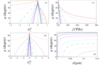
Figure 2: (Color online) Leaky wave launch angle, $\varphi$, as a function of permittivity, $\epsilon_{2}^{xx}$ (Figs. (a) and (b)) for eight different thicknesses in succession, starting with $d=1$ µm (dotted orange curve), and subsequent values of $d$ (in µm), equaling $1/5,1/10,1/20,1/30,1/40,1/50$, and $1/60$. Other parameters are as in Fig. 1. In (c) the emission angle is shown as a function of frequency for the same thicknesses in (a) and (b). In (d), the effects of geometrical variation are presented for $\epsilon_{2}^{xx}=0.001,0.01,0.05,0.2,0.4,0.6$, and $0.8$. The curves with larger overall $\varphi$ correspond to smaller $\epsilon_{2}^{xx}$ in succession.

Next, in Fig. 2, we show the angle, $\varphi$, which defines the radiation cone from the surface of the metamaterial structure, as functions of both $\epsilon_{2}^{xx}$, frequency, and thickness parameter $d$. In panel (a), the variation in $\varphi$ is shown over a broad range of $\epsilon_{2}^{xx}$ for nonmagnetic media ($\mu_{2}^{yy}=1$), while panel (b) is for a metamaterial with vanishing $\mu_{2}^{yy}$, representative of a type of matched impedance cuong . The eight curves in Fig. 2 (a) and (b) represent different widths, identified in the caption. We see that for $\epsilon_{2}^{xx}\rightarrow 0$, we recover the isotropic result of nearly normal emission ($\varphi\approx 90^{\rm o}$), discussed and demonstrated in the millimeter regime enoch . This behavior can be understood in our system, at least qualitatively, from a geometrical optics perspective and a generalization of Snell’s Law for bianisotropic media kong . When the magnetic response vanishes (Fig. 2 (b)), the emission angle becomes symmetric with respect to $\epsilon_{2}^{xx}$, dropping from $\varphi=\pi/2$ for zero $\epsilon_{2}^{xx}$, to broadside ($\varphi=0$) when $\epsilon_{2}^{xx}=\pm 4k_{0}d$. Thus thinner widths result in more rapid beam variation as a function of $\epsilon_{2}^{xx}$. In Fig. 2(c) we show how the emission angle varies as a function of frequency, with the transverse response obeying the Drude form, $\epsilon_{2}^{xx}=1-\omega_{p}^{2}/(\omega^{2}+i\Gamma\omega)$. Here, $\omega_{p}=(2\pi)120$ THz and $\Gamma=0$, to isolate leaky wave effects. With increasing frequency, we observe similar trends found in the previous figures, where a larger dielectric response pulls the beam towards the metamaterial. In (d), a geometrical study illustrates how the emission angle varies with thickness: for $\epsilon_{2}^{xx}\mu_{2}^{yy}<1$, the emission angle rises abruptly with increased $d$, before leveling off at $\phi=\tan^{-1}(\sqrt{1/(\epsilon_{2}^{xx}\mu_{2}^{yy})-1})$. Physically, as the slab increases in size, the complex propagation constant becomes purely real, $\gamma\rightarrow\sqrt{\epsilon_{2}^{xx}\mu_{2}^{yy}}$, and $q^{+}\rightarrow\sqrt{1-\epsilon_{2}^{xx}\mu_{2}^{yy}}$. This is consistent with what was discussed previously involving the depletion of $\alpha$ with $d$; for thick ENZ slabs, leaky wave radiation is replaced by conventional propagating modes. For fixed $\epsilon_{2}^{xx}$, there is also a critical thickness, $d^{*}$, below which no leaky waves are emitted, which by Eq. (3) is, $d^{*}=\epsilon_{2}^{xx}/(4k_{0}\sqrt{1-\epsilon_{2}^{xx}\mu_{2}^{yy}})$.

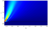
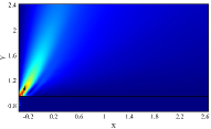
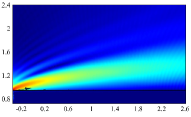
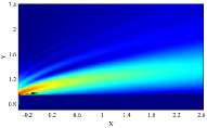
Figure 3: Normalized field profiles illustrating broad angular variation in beam emission. The arrows along the interfaces depict the Poynting vector. The top left and right panels correspond to $\epsilon_{2}^{xx}=0.05$, and $\epsilon_{2}^{xx}=0.05+0.02i$, respectively. The the bottom left and right panels are for $\epsilon_{2}^{xx}=0.66$ and $\epsilon_{2}^{xx}=0.66+0.02i$, respectively. The metamaterial is subwavelength ($d=1/20$ µm) and nonmagnetic ($\mu_{2}^{yy}=1$). Coordinates are given in units of $(\times 10)$ µm.

These results are consistent with simulations from a commercial finite element software package comsol . In Fig. 3, we show the normalized $|{\bm{H}}|$ arising from a source excitation (at $f=280$ THz) within the metamaterial for $d=1/20$ µm. The left two panels are for $\Gamma=0$, and the right two have absorption present. The full wave simulations agree with Fig. 2(a) (dashed green curve), where the leaky-wave energy outflow spans a broad angular range when $0\lesssim\epsilon_{2}^{xx}\lesssim 0.68$. The right two panels exemplify the robustness of this effect for moderate amounts of loss present in the metamaterial.

In conclusion, we have demonstrated leaky wave radiation in subwavelength biaxial metamaterials with vanishing permittivity along the longitudinal direction. The leaky-wave radiation cone illustrated broad directionality through variations in the transverse EM response. By utilizing nanodeposition techniques, such structures can be fabricated by implementing an array of metallic nanowires embedded in a self-organized porous nanostructured material alek .

- (1) X. Liu, et al., Phys. Rev. Lett. , 104, 207403 (2010).
- (2) S. Zhang, et al., Phys. Rev. Lett. , 102, 023901 (2009).
- (3) C. Menzel, et al., Phys. Rev. Lett. , 104, 253902 (2010).
- (4) R.W. Ziolkowski, Phys. Rev. E70, 046608 (2004).
- (5) V. C. Nguyen, et al., Phys. Rev. Lett. 105, 233908 (2010).
- (6) S. Enoch, et al., Phys. Rev. Lett. 89, 213902 (2002).
- (7) M. Silveirinha and N. Engheta, Phys. Rev. Lett. 97, 157403 (2006).
- (8) A. Alù, et al., Phys. Rev. B, 65, 155410 (2007).
- (9) M. Laroche, et al., Phys. Rev. Lett. 96, 123903 (2006).
- (10) N.-H. Shen, et al., Phys. Rev. Lett. , bf 106, 037403 (2011).
- (11) S. Zhang, et al., Phys. Rev. Lett. , 95, 137404 (2005).
- (12) N.-H. Shen, et al., Phys. Rev. Lett. 106, 037403 (2011).
- (13) L.V. Alekseyev, et al., Appl. Phys. Lett. 97, 131107 (2010).
- (14) X-X. Liu and A. Alù, Phys. Rev. B82 144305 (2010).
- (15) V. Mocella, et al., Opt. Express 18, 25068 (2010).
- (16) V.A. Podolskiy and E.E. Narimanov, Phys. Rev. B, 71, 201101(R) (2005).
- (17) I. I. Smolyaninov, et al., Phys. Rev. Lett. 102, 213901 (2009).
- (18) R. E. Collin and F. J. Zucker, Antenna Theory, Part II, Mcgraw-Hill (1969).
- (19) T. Tamir and F. Y. Kou, IEEE J. Quantum Electr. 22, 544 (1986).
- (20) E. Colak, et al., Optics Express 17, 9879 (2009).
- (21) A. Micco, et al., Phys. Rev. B79, 075110 (2009).
- (22) S. Lim, IEEE trans. on Microw. theory and Tech. 52, 2678 (2004).
- (23) P. Baccarelli, et al., IEEE Trans. on Microw. Th. and Tech., 53, 32 (2005).
- (24) Y. Yuan, et al., Phys. Rev. A77, 053821 (2008).
- (25) H. Liu and K. J. Webb, Phys. Rev. B 81, 201404(R) (2010).
- (26) R. Loudon, J. Phys A 3, 233 (1970).
- (27) R. Ruppin, Phys. Lett. A 299, 309 (2002).
- (28) L. D. Landau, E. M. Lifshitz, and L. P. Pitaevskii, Electrodynamics of Continuous Media (Butterworth-Heinemann, Oxford, 1984), 2nd ed.
- (29) T. M. Grzegorczyk, et al., IEEE Trans. On Microw. Theory and Tech. 53, 1443 (2005).
- (30) COMSOL Multiphysics, http://www.comsol.com