Improved Mixing Condition on the Grid for Counting and Sampling Independent Sets

Abstract

The hard-core model has received much attention in the past couple of decades as a lattice gas model with hard constraints in statistical physics, a multicast model of calls in communication networks, and as a weighted independent set problem in combinatorics, probability and theoretical computer science.

In this model, each independent set $I$ in a graph $G$ is weighted proportionally to $\lambda^{|I|}$, for a positive real parameter $\lambda$. For large $\lambda$, computing the partition function (namely, the normalizing constant which makes the weighting a probability distribution on a finite graph) on graphs of maximum degree $\Delta\geq 3$, is a well known computationally challenging problem. More concretely, let $\lambda_{c}(\mathbb{T}_{\Delta})$ denote the critical value for the so-called uniqueness threshold of the hard-core model on the infinite $\Delta$-regular tree; recent breakthrough results of Dror Weitz (2006) and Allan Sly (2010) have identified $\lambda_{c}(\mathbb{T}_{\Delta})$ as a threshold where the hardness of estimating the above partition function undergoes a computational transition.

We focus on the well-studied particular case of the square lattice $\mathbb{Z}^{2}$, and provide a new lower bound for the uniqueness threshold, in particular taking it well above $\lambda_{c}(\mathbb{T}_{4})$. Our technique refines and builds on the tree of self-avoiding walks approach of Weitz, resulting in a new technical sufficient criterion (of wider applicability) for establishing strong spatial mixing (and hence uniqueness) for the hard-core model. Our new criterion achieves better bounds on strong spatial mixing when the graph has extra structure, improving upon what can be achieved by just using the maximum degree. Applying our technique to $\mathbb{Z}^{2}$ we prove that strong spatial mixing holds for all $\lambda<{2.3882}$, improving upon the work of Weitz that held for $\lambda<27/16=1.6875$. Our results imply a fully-polynomial deterministic approximation algorithm for estimating the partition function, as well as rapid mixing of the associated Glauber dynamics to sample from the hard-core distribution.

1 Introduction

In this paper we study phase transitions for sampling weighted independent sets (weighted by an activity $\lambda>0$) of the 2-dimensional integer lattice $\mathbb{Z}^{2}$. In statistical physics terminology, we study the hard-core lattice gas model ([6, 13]), which is a simple model of a gas whose particles have non-negligible size (thus preventing them from occupying neighboring sites), with activity $\lambda\in\mathbb{R}_{+}$ corresponding to the so-called fugacity of the gas. More formally, for a finite graph $G=(V,E)$, let $\Omega=\Omega(G)$ denote the set of independent sets of $G$. Given an independent set $\sigma\in\Omega$, its weight is defined as $w(\sigma)=\lambda^{|\sigma|}$ and $v\in V$ is said to be occupied under $\sigma$ if $v\in\sigma$. The associated Gibbs (or Boltzmann) distribution $\mu=\mu_{G,\lambda}$ is defined on $\Omega$ as $\mu(\sigma)=w(\sigma)/Z$, where $Z=Z(G,\lambda)=\sum_{\eta\in\Omega}w(\eta)$ is commonly referred to as the partition function.

Recall that Valiant [33] showed that exactly computing the number of independent sets is #P-complete, even when restricted to 3-regular graphs (see Greenhill [16]). Hence, we focus our attention on approximation algorithms for estimating the number, or more generally, the partition function. It is well known [17] that the problem of approximating the partition function $Z$ and that of sampling from a distribution that is close to the Gibbs distribution $\mu$, are polynomial-time reducible to each other (see also [31]).

The fundamental notion of a phase transition for a statistical mechanics model on an infinite graph addresses the critical point at which the model starts to exhibit a certain long-range dependence, as a system parameter is varied. In particular, the so-called critical inverse temperature $\beta_{c}$ for the Ising or the Potts model, and the critical activity $\lambda_{c}$ for the hard-core lattice gas model, are prime examples where the system undergoes a transition from uniqueness to multiplicity of the infinite-volume Gibbs measures.

Phase transition in the hard-core model is also intimately related to the computational complexity of estimating the partition function $Z$. Recently, a remarkable connection was established between the computational complexity of approximating the partition function for graphs of maximum degree $\Delta$ and the phase transition $\lambda_{c}(\mathbb{T}_{\Delta})$ for the infinite regular tree $\mathbb{T}_{\Delta}$ of degree $\Delta$. On the positive side, Weitz [34] showed a deterministic fully-polynomial time approximation algorithm (FPAS) for approximating the partition function for any graph with maximum degree $\Delta$, when $\lambda<\lambda_{c}(\mathbb{T}_{\Delta})$ and $\Delta$ is constant. On the other side, Sly [30] recently showed that for every $\Delta\geq 3$, it is NP-hard (unless NP=RP) to approximate the partition function for graphs of maximum degree $\Delta$, when $\lambda_{c}(\mathbb{T}_{\Delta})<\lambda<\lambda_{c}(\mathbb{T}_{\Delta})+\epsilon_{\Delta}$, for some function $\epsilon_{\Delta}>0$. More recently, Galanis et al. [12] improved the range of $\lambda$ in Sly’s inapproximability result, extending it to all $\lambda>\lambda_{c}(\mathbb{T}_{\Delta})$ for the cases $\Delta=3$ and $\Delta\geq 6$.

1.1 Prior history and current work

Our work builds upon Weitz’s work to get improved results for specific graphs of interest. We focus our attention on what is arguably the simplest, not yet well-understood, case of interest namely the square grid, or the 2-dimensional integer lattice $\mathbb{Z}^{2}$. Empirical evidence suggests that the critical point $\lambda_{c}(\mathbb{Z}^{2})\approx 3.796$ [13, 3, 26], but rigorous results are significantly far from this conjectured point. The possibility of there being multiple such $\lambda_{c}$ is not ruled out, although no one believes that this is the case.

From below, van den Berg and Steif [6] used a disagreement percolation argument to prove $\lambda_{c}(\mathbb{Z}^{2})>\frac{p_{c}}{1-p_{c}}$ where $p_{c}$ is the critical probability for site percolation on $\mathbb{Z}^{2}$. Applying the best known lower bound on $p_{c}>0.556$ for $\mathbb{Z}^{2}$ by van den Berg and Ermakov [5] implies $\lambda_{c}(\mathbb{Z}^{2})>1.252\dots$. Prior to that work, an alternative approach aimed at establishing the Dobrushin-Shlosman criterion [10], yielded, via computer-assisted proofs, $\lambda_{c}(\mathbb{Z}^{2})>1.185$ by Radulescu and Styer [28], and $\lambda_{c}(\mathbb{Z}^{2})>1.508$ by Radulescu [27].

These results were improved upon by Weitz [34] who showed that $\lambda_{c}(\mathbb{Z}^{2})\geq\lambda_{c}(\mathbb{T}_{4})=27/16=1.6875$, where $\mathbb{T}_{\Delta}$ is the infinite, complete, regular tree of degree $\Delta$. For the upper bound, a classical Peierls’ type argument implies $\lambda_{c}(\mathbb{Z}^{2})=O(1)$ [9]. (A related result of Randall [29] showing slow mixing of the Glauber dynamics for $\lambda>8.066$ gives hope for a better upper bound on $\lambda_{c}(\mathbb{Z}^{2})$.) The regular tree $\mathbb{T}_{\Delta}$ is one of the only examples (that we know of) where the critical point is known exactly, and in this case, Kelly [18] showed that $\lambda_{c}(\mathbb{T}_{\Delta})=(\Delta-1)^{\Delta-1}/(\Delta-2)^{\Delta}$.

In this work we present a new general approach which, for the case of the hard-core model on $\mathbb{Z}^{2}$, improves the lower bound to $\lambda_{c}(\mathbb{Z}^{2})>{2.3882}$. There are various algorithmic implications for finite subgraphs of the $\mathbb{Z}^{2}$ when $\lambda<{2.3882}$. Our results imply that Weitz’s deterministic FPAS is also valid on subgraphs of $\mathbb{Z}^{2}$ for the same range of $\lambda$. Thanks to the existing literature on general spin systems ([22, 23, 8, 11]), our results also imply that the Glauber dynamics has $O(n\log{n})$ mixing time for any finite subregion $G=(V,E)$ of $\mathbb{Z}^{2}$ when $\lambda<{2.3882}$, where $n=|V|$. Recall that the Glauber dynamics is a simple Markov chain that updates the configuration at a randomly chosen vertex in each step, see [19] for an introduction to the Glauber dynamics. The stationary distribution of this chain is the Gibbs distribution. Hence, it is of interest as an algorithmic technique to randomly sample from the Gibbs distribution, and also as a model of how physical systems reach equilibrium. The mixing time is the number of steps (from the worst initial configuration) until the distribution is guaranteed to be within variation distance $\leq 1/4$ of the stationary distribution.

As in Weitz’s work, our approach can be used for other 2-spin systems, such as the Ising model. This is discussed in Section 6. As will be evident from the following high-level idea of our approach, it can be applied to other graphs of interest. Our work also provides an arguably simpler way to derive the main technical result of Weitz showing that any graph with maximum degree $\Delta$ has strong spatial mixing (SSM) when $\lambda<\lambda_{c}(\mathbb{T}_{\Delta})$.

To underline the difficulty in estimating bounds on $\lambda_{c}$, we remark that the existence of a (unique) critical activity $\lambda_{c}$ remains conjectural and an open problem for $\mathbb{Z}^{d}$, for $d\geq 2$. In contrast, for the Ising model, the critical inverse temperature $\beta_{c}(\mathbb{Z}^{2})$ has been known since 1944 [24]; interestingly, the corresponding critical point for the $q$-state Potts model (for $q\geq 2$) has only recently been established (by Beffara and Duminil-Copin [4]) to be $\beta_{c}(q)=\log(1+\sqrt{q})$, settling a long-standing open problem. The lack of monotonicity in $\lambda$ in the hard-core model poses a serious challenge in establishing such a sharp result for this model. In fact, Brightwell et al. [7] showed that in general such a monotonicity need not hold, by providing an example with a non-regular tree.

2 Technical Preliminaries and Proof Approach

Before presenting our approach, it is useful to review briefly the uniqueness/non-uniqueness phase transition, and introduce associated notions of decay of spatial correlation, known as weak and strong spatial mixing properties. Much of the below discussion is simplified for the case of the hard-core model on $\mathbb{Z}^{2}$, wherein one utilizes certain induced monotonicity (given by the bipartite property) in the model and the amenability of the graph.

2.1 Uniqueness, Weak and Strong Spatial Mixing

Let $B_{L}$ denote the finite graph corresponding to a box of side-length $2L+1$ centered around the origin in $\mathbb{Z}^{2}$. Thus, $B_{L}=(V,E)$, where $V={(i,j)\in\mathbb{Z}^{2}:-2L-1\leq i,j\leq 2L+1}$ with edges between pairs of vertices at $L_{1}$ distance (or Manhattan distance) equal to one. Since this is a bipartite graph, we may fix one such partition $V=\mathrm{even}\cup\mathrm{odd}$ – for example, it is standard to consider the set of vertices at an even distance from the origin as the even set. The boundary of $B_{L}$ are those vertices $v=(v_{1},v_{2})\in V$ where $|v_{i}|=2L+1$ for $i=1$ or $i=2$. The hard-core model on bipartite graphs is a monotone system (e.g., see [11]), which for the current discussion implies that we only have to consider two assignments to the boundary: all even vertices or all odd vertices on the boundary are occupied. Let $\alpha_{L,r}^{\mathrm{even}}$ ($\alpha_{L,r}^{\mathrm{odd}}$) denote the marginal probability that the origin $r$ is unoccupied given the even (odd, respectively) boundary. Then to establish uniqueness of the Gibbs measures, we need that:

$$\lim_{L\rightarrow\infty}|\alpha_{L,r}^{\mathrm{even}}-\alpha_{L,r}^{\mathrm{odd}}|=0.$$

We are interested in the critical point $\lambda_{c}$ for the transition between uniqueness and non-uniqueness. A standard way to establish uniqueness is by proving one of the spatial mixing properties introduced next.

Let $G=(V,E)$ be a (finite) graph. For $S\subset V$, a configuration $\boldsymbol{\rho}$ on $S$ specifies a subset of $S$ as occupied and the remainder as unoccupied. Let $\mu^{\boldsymbol{\rho}}=\mu^{\boldsymbol{\rho}}_{G}$ denote the Gibbs distribution conditional on configuration $\boldsymbol{\rho}$ to $S$. For $v\in V$, let $\alpha^{\boldsymbol{\rho}}_{v}=\alpha_{G,v}^{\boldsymbol{\rho}}$ denote the marginal probability that $v$ is unoccupied in $\mu^{\boldsymbol{\rho}}$.

The first spatial mixing property is Weak Spatial Mixing (WSM). Here we consider a pair of boundary configurations on a subset $S$ and consider the “influence” on the marginal probability that a vertex $v$ is unoccupied. WSM says that the influence on $v$ decays exponentially in the distance of $S$ from $v$.

Definition 1 (Weak Spatial Mixing).

For the hard-core model at activity $\lambda$, for finite graph $G=(V,E)$, WSM holds with rate $\gamma\in(0,1)$ if for every $v\in V$, every $S\subset V$, and every two configurations $\boldsymbol{\rho},\boldsymbol{\eta}$ on $S$,

$$\left|\alpha^{\boldsymbol{\rho}}_{v}-\alpha^{\boldsymbol{\eta}}_{v}\right|~{}\leq~{}\gamma^{\mathrm{dist}(v,T)}$$

where $\mathrm{dist}(v,S)$ is the graph distance (i.e., length of the shortest path) between $v$ and (the nearest point in) the subset $S$.

The second property of interest is Strong Spatial Mixing (SSM). The intuition is that if a pair of boundary configurations on a subset $S$ agree at some vertices in $S$ then those vertices “encourage” $v$ to agree. Therefore, SSM says that the influence on $v$ decays exponentially in the distance of $v$ from the subset of vertices where the pair of configurations differ.

Definition 2 (Strong Spatial Mixing).

For the hard-core model at activity $\lambda$, for finite graph $G=(V,E)$, SSM holds with rate $\gamma\in(0,1)$ if for every $v\in V$, every $S\subset V$, every $S^{\prime}\subset S$, and every two configurations $\boldsymbol{\rho},\boldsymbol{\eta}$ on $S$ where $\boldsymbol{\rho}(S\setminus S^{\prime})=\boldsymbol{\eta}(S\setminus S^{\prime})$,

$$\left|\alpha^{\boldsymbol{\rho}}_{v}-\alpha^{\boldsymbol{\eta}}_{v}\right|~{}\leq~{}\gamma^{\mathrm{dist}(v,S^{\prime})}.$$

Note that since $\mathrm{dist}(v,T)\leq\mathrm{dist}(v,T\setminus S)$, SSM implies WSM for the same rate. Moreover, it is a standard fact that such an exponential decay in finite boxes (say), in $\mathbb{Z}^{d}$, implies uniqueness of the corresponding infinite volume Gibbs measure on $\mathbb{Z}^{d}$, see Georgii [14] for an introduction to the theory of infinite-volume Gibbs measures. We can specialize the above notions of WSM and SSM to a particular vertex $v$, in which case we say that WSM or SSM holds at $v$. If the graph is a rooted tree, we will always assume that the notions of WSM and SSM are considered at the root.

For the hard-core model on a graph $G=(V,E)$, for a subset of vertices $S$ and a fixed configuration $\rho$ on $S$, it is equivalent to consider the subgraph $G^{\prime}$ which we obtain for each $v\in S$ that is fixed to be unoccupied we remove $v$ from $G$, and for each $v\in S$ that is fixed to be occupied we remove $v$ and its neighbors $N(v)$ from $G$. In this way we obtain the following observation which will be useful for proving SSM holds.

Observation 1.

For a graph $G=(V,E)$ and $v\in V$, SSM holds in $G$ at vertex $v$ iff WSM holds for all subgraphs $G^{\prime}$ (of $G$) at vertex $v$. To be precise, by subgraphs we mean graphs obtained by considering all subgraphs of $G$ and taking the component containing $v$.

2.2 Self-Avoiding Walk Tree Representation

Since our work builds on that of Weitz’s, we first describe the self-avoiding walk (SAW) tree representation introduced in [34]. Given $G=(V,E)$, we first fix an arbitrary ordering $>_{w}$ on the neighbors of each vertex $w$ in $G$. For each $v\in V$, the tree $T_{\mathrm{saw}}(G,v)$ is constructed as follows. Consider the tree $T$ of self-avoiding walks originating from $v$, additionally including the vertices closing a cycle as leaves of the tree. We then fix such leaves of $T$ to be occupied or unoccupied in the following manner. If a leaf vertex closes a cycle in $G$, say $w\to v_{1}\to\dots v_{\ell}\to w$, then if $v_{1}>_{w}v_{\ell}$ we fix this leaf to be unoccupied, otherwise if $v_{1}<_{w}v_{\ell}$ we fix the leaf to be occupied. Note, if the leaf is fixed to be unoccupied we simply remove that vertex from the tree. If the leaf is fixed to be occupied, we remove that leaf and all of its neighbors, i.e. we remove the parent of that leaf from the tree. The resulting tree is denoted as $T_{\mathrm{saw}}=T_{\mathrm{saw}}(G,v)$. See Figure 1 for an illustration of $T_{\mathrm{saw}}$ for a particular example.

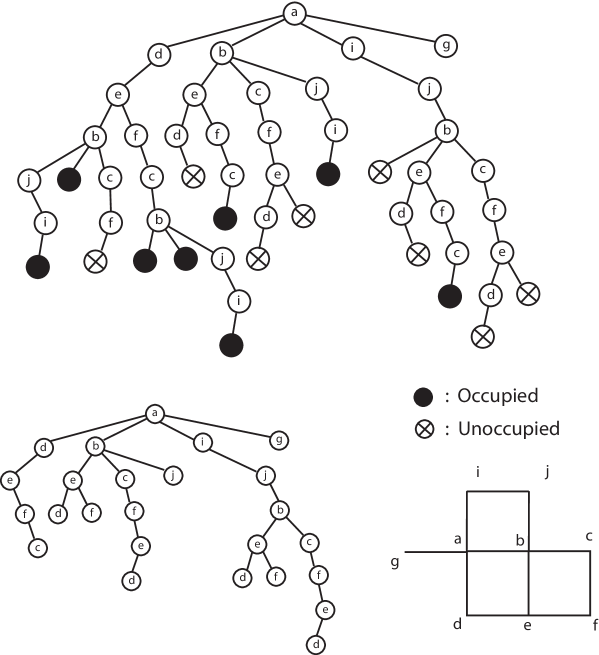
Figure 1: Example of self-avoiding walk tree $T_{\mathrm{saw}}$. The above tree describes $T_{\mathrm{saw}}(G,a)$ with occupied and unoccupied leaves, while the below one is the same tree after removing those assigned leaves. At each vertex, we consider the ordering $N>E>S>W$ of its neighbors where $N,E,S,W$ represent the neighbors in the North, East, South, West directions, respectively.

Weitz [34] proves the following theorem for the hard-core model, which shows that the marginal distribution at the root in $T_{\mathrm{saw}}(G,v)$ is identical to the marginal distribution for $v$ in $G$. For a graph $G=(V,E)$, a subset $S\subset V$ and configuration $\rho$ on $S$, for $T_{\mathrm{saw}}=T_{\mathrm{saw}}(G,v)$, let $\rho$ in $T_{\mathrm{saw}}$ denote the configuration on $S$ in $T_{\mathrm{saw}}$ where for $w\in S$ every occurrence of $w$ in $T_{\mathrm{saw}}$ is assigned according to $\rho$.

Theorem 1 (SAW Tree Representation, Theorem 3.1 in [34]).

For any graph $G=(V,E)$, $v\in V$, $\lambda>0$, and configuration $\boldsymbol{\rho}$ on $S\subset V$, for $T=T_{\mathrm{saw}}(G,v)$ the following holds:

$$\alpha_{G,v}^{\boldsymbol{\rho}}=\alpha_{T,v}^{\boldsymbol{\rho}}.$$

Note, the tree $T_{\mathrm{saw}}(G,v)$ preserves the distance of vertices from $v$ in $G$, which implies the following corollary.

Corollary 2.

If SSM holds with rate $\gamma$ for $T_{\mathrm{saw}}(G,v)$ for all $v$, then SSM holds for $G$ with rate $\gamma$.

The reverse implication of Corollary 2 does not hold since there are configurations on $S$ in $T_{\mathrm{saw}}$ which are not necessarily realizable in $G$. Observe that if $G$ has maximum degree $\Delta$, any SAW tree of $G$ is a subtree of the regular tree of degree $\Delta$.

2.3 Our Proof Approach

In summary, Weitz [34] first shows (via Theorem 1) that to prove SSM holds on a graph $G=(V,E)$, it suffices to prove SSM holds on the trees $T_{\mathrm{saw}}(G,v)$, for all $v\in V$. Weitz then proves that the regular tree $\mathbb{T}_{\Delta}$ “dominates” every tree of maximum degree $\Delta$ in the sense that, for all trees of maximum degree $\Delta$, SSM holds when $\lambda<\lambda_{c}(\mathbb{T}_{\Delta})$. We refine this second part of Weitz’s approach. In particular, for graphs with extra structure, such as $G=\mathbb{Z}^{2}$, we bound $T_{\mathrm{saw}}(\mathbb{Z}^{2})$ by a tree $T^{*}$ that is much closer to it than the regular tree $\mathbb{T}_{\Delta}$. We then establish a criterion that achieves better bounds on SSM for trees when the trees have extra structure.

The tree $T^{*}$ will be constructed in a regular manner so that we can prove properties about it – the construction of $T^{*}$ is governed by a (progeny) $t\times t$ matrix $\boldsymbol{M}$, whose rows correspond to $t$ types of vertices, with the entry $M_{ij}$ specifying the number of children of type $j$ that a vertex of type $i$ begets. We will then show a sufficient condition using entries of $\boldsymbol{M}$ which implies that SSM holds for $T^{*}$ and for any subgraph of $T^{*}$, including $T_{\mathrm{saw}}(\mathbb{Z}^{2})$. The construction of $T^{*}$ is reminiscent of the strategy employed in [1, 25] to upper bound the connectivity constant of several lattice graphs, including $\mathbb{Z}^{2}$. The derivation of our sufficient condition has some inspiration from belief propagation algorithms.

As a byproduct of our proof that our new criterion implies SSM for $T^{*}$, we get a new (and simpler) proof of the second part of Weitz’s approach, namely, that for all trees of maximum degree $\Delta$, SSM holds when $\lambda<\lambda_{c}(\mathbb{T}_{\Delta})$.

3 Branching Matrices and Strong Spatial Mixing

As alluded to above, we will utilize more structural properties of self-avoiding walk trees. To this end, we consider families of trees which can be recursively generated by certain rules; we then show that such a general family is also analytically tractable.

3.1 Definition of Branching Matrices

We say that the matrix $\boldsymbol{M}$ is a $t\times t$ branching matrix if every entry $M_{ij}$ is a non-negative integer. We say the maximum degree of $\boldsymbol{M}$ is $\Delta=\Delta(\boldsymbol{M})=\max_{1\leq i\leq t}\sum_{1\leq j\leq t}M_{ij}$, the maximum row sum. Given a branching matrix $\boldsymbol{M}$, we define the following family of graphs. In essence, it includes a graph $G$ if the self-avoiding walk trees of $G$ can be generated by $\boldsymbol{M}$.

Definition 3 (Branching Family).

Given a $t\times t$ branching matrix $\boldsymbol{M}$, $\mathcal{F}_{\leq\boldsymbol{M}}$ includes trees which can be generated under the following restrictions:

• Each vertex in tree $T\in\mathcal{F}_{\leq\boldsymbol{M}}$ has its type $i\in\{1,\dots,t\}$.

• Each vertex of type $i$ has at most $M_{ij}$ children of type $j$.

In addition, we use the notation $G=(V,E)\in\mathcal{F}_{\leq\boldsymbol{M}}$ if $T_{\mathrm{saw}}(G,v)\in\mathcal{F}_{\leq\boldsymbol{M}}$ for all $v\in V$.

For example, the family $\mathcal{F}_{\leq\boldsymbol{M}}$ with $\boldsymbol{M}=[\Delta]$ includes the family of trees with maximum branching $\Delta$. On the other hand, $\mathcal{F}_{\leq\boldsymbol{M}}$ with $\boldsymbol{M}=\begin{pmatrix}0&\Delta+1\\ 0&\Delta\end{pmatrix}$ describes the family of graphs of maximum degree $\Delta+1$, by assigning the root of tree $T\in\mathcal{F}_{\leq\boldsymbol{M}}$ to be of type 1 and the other vertices of the tree to be of type 2. Note that if $\boldsymbol{M}$ has maximum degree $\Delta$, then every $G\in\mathcal{F}_{\leq\boldsymbol{M}}$ also has maximum degree $\Delta$.

In this framework, Weitz’s result establishing SSM for all graphs of maximum degree $\Delta$ when $\lambda<\lambda_{c}(\mathbb{T}_{\Delta})$ can be stated as establishing SSM with uniform rate for all $G\in\mathcal{F}_{\leq\boldsymbol{M}}$ with $\boldsymbol{M}=\begin{pmatrix}0&\Delta\\ 0&\Delta-1\end{pmatrix}$; and we are interested in establishing its analogy for general $\boldsymbol{M}$. To this end, we will use the following notion of SSM for $\boldsymbol{M}$.

Remark 1.

To establish SSM for $\boldsymbol{M}$, it suffices to prove that SSM holds with uniform rate for all trees in $\mathcal{F}_{\leq\boldsymbol{M}}$ due to Corollary 2. In addition, note that SSM holds for $\boldsymbol{M}=\begin{pmatrix}0&\Delta+1\\ 0&\Delta\end{pmatrix}$ if and only if it holds for $(\Delta)$ since the root of a tree $T\in\mathcal{F}_{\leq\boldsymbol{M}}$ is the only possible vertex of type 1 in $T$.

Finally, we define SSM for a branching matrix $\boldsymbol{M}$.

Definition 4.

Given a branching matrix $\boldsymbol{M}$, we say SSM holds for $\boldsymbol{M}$ if SSM holds with uniform rate for all $G\in\mathcal{F}_{\leq\boldsymbol{M}}$.

Remark 2.

To establish SSM for $\boldsymbol{M}$, it suffices to prove that SSM holds with uniform rate for all trees in $\mathcal{F}_{\leq\boldsymbol{M}}$ due to Corollary 2.

3.2 Implications of SSM

We present a new approach for proving SSM for a branching matrix $\boldsymbol{M}$. There are multiple consequences of SSM for $\boldsymbol{M}$ as summarized in the following theorem. We first state some definitions needed for stating the theorem.

Following Goldberg et al. [15] we use the following variant of amenability for infinite graphs. Here we consider an infinite graph $G=(V,E)$. For $v\in V$ and a non-negative integer $d$, let $\mathrm{B}_{d}(v)$ denote the set of vertices within distance $\leq d$ from $v$, where distance is the length of the shortest path. For a set of vertices $S$, the (outer) boundary and neighborhood amenability are defined, respectively, as:

$$\partial S:=\{w\in V:w\notin S,\mbox{ and $w$ has a neighbor $y\in S$}\}\ \ \mbox{ and }\ \ r_{d}=\sup_{v\in V}\frac{|\partial\mathrm{B}_{d}(v)|}{|\mathrm{B}_{d}(v)|}\,.$$

The infinite graph is said to be neighborhood-amenable if $\inf_{d}r_{d}=0$.

Now we can state the following theorem detailing the implications of SSM of interest to us.

Theorem 3.

For a $t\times t$ branching matrix $\boldsymbol{M}$, if SSM holds for $\boldsymbol{M}$ then the following hold:

1. For every $G\in\mathcal{F}_{\leq\boldsymbol{M}}$, SSM holds on $G$.

2. For every infinite graph $G\in\mathcal{F}_{\leq\boldsymbol{M}}$, there is a unique infinite-volume Gibbs measure on $G$.

3. If $\boldsymbol{M}$ has maximum degree $\Delta$, if $t=O(1)$ and $\Delta=O(1)$, then for every (finite) $G\in\mathcal{F}_{\leq\boldsymbol{M}}$, Weitz’s algorithm [34] gives an FPAS for approximating the partition function $Z(G)$.

4. For every infinite $H\in\mathcal{F}_{\leq\boldsymbol{M}}$ which is neighborhood-amenable, for every finite subgraph $G=(V,E)$ of $H$, the Glauber dynamics has $O(n^{2})$ mixing time. Moreover, if $H=\mathbb{Z}^{d}$ for constant $d$, then for every finite subgraph $G=(V,E)$ of $H$, the Glauber dynamics has $O(n\log{n})$ mixing time.

Proof.

Part 1 is by the definition of SSM for $\boldsymbol{M}$. The uniqueness result follows from the fact that the infinite-volume extremal Gibbs measures on the infinite graph $G$ can be obtained by taking limits of finite measures, see Georgii [14] for an introduction to infinite-volume Gibbs measures, and see Martinelli [21] for Part 2. Part 3 immediately follows from the work of Weitz [34]. Finally, for Part 4, there is a long line of work showing that for the integer lattice $\mathbb{Z}^{d}$ in fixed dimensions, for the Ising model SSM on $\mathbb{Z}^{d}$ implies $O(n\log{n})$ mixing time of the Glauber dynamics on finite subregions of $\mathbb{Z}^{d}$, e.g., see Cesi [8] and Martinelli [21] (and the references therein) for recent results on this problem. These results for the Ising model are typically stated for a general class of models, but that class does not include models with hard constraints, such as the hard-core model studied here. Dyer et al. [11] showed a simpler proof for the hard-core model that utilizes the monotonicity of the model. We use this result of [11] in Theorem 8 to get $O(n\log{n})$ mixing time for subregions of $\mathbb{Z}^{2}$. Goldberg et al. [15, Theorem 8] showed that for $k$-colorings, if SSM holds for an infinite graph $G$ that is neighborhood-amenable, the Glauber dynamics has $O(n^{2})$ mixing time for all finite subgraphs of $G$. Their proof holds for the hard-core model which implies Part 4. ∎

4 Establishing SSM for Branching Matrices

In this section we present a sufficient condition implying SSM for the family of trees generated by a branching matrix. As a consequence of the approach presented in this section we get a simpler proof of Weitz’s result [34] implying SSM for all graphs with maximum degree $\Delta$ when $\lambda<\lambda_{c}(\mathbb{T}_{\Delta})$. We then apply the condition presented in this section to $\mathbb{Z}^{2}$ in Section 5.

To show the decay of influence of a boundary condition $\boldsymbol{\rho}$, a common strategy is to prove some form of contraction for the ‘one-step’ iteration given in (1) below. More generally, we will prove such a contraction for an appropriate set of ‘statistics’ of the unoccupied marginal probability.

A statistic of the univariate parameter $x\in[a,b]$ is a monotone (i.e., strictly increasing or decreasing) function $\varphi:[a,b]\rightarrow\mathbb{R}$. For a $t\times t$ branching matrix $\boldsymbol{M}$ we consider a set of $t$ statistics $\varphi_{1},\dots,\varphi_{t}$, one for each type. For the simpler case when $\boldsymbol{M}=[\Delta]$ and hence $t=1$, we have a single statistic $\varphi$. Our aim is proving contraction for an appropriate set of statistics of the probability that the root of a tree is unoccupied.

We first focus on the case of a single type. Consider a tree $T=(V,E)\in\mathcal{F}_{\leq\boldsymbol{M}}$ with root $r$. For $v\in V$, let $N(v)$ denote the children of $v$, and let $d(v):=|N(v)|$ the number of children. Let $T_{v}$ denote the subtree rooted at $v$. We will analyze the unoccupied probability for a vertex $v$, but $v$ will always be the root of its subtree. Hence, to simplify the notation, for a boundary condition $\boldsymbol{\rho}$ on $S\subset V$, let $\alpha_{v}^{\boldsymbol{\rho}}=\alpha_{T_{v},v}^{\boldsymbol{\rho}}$.

A straightforward recursive calculation with the partition function leads to the following relation:

$$\alpha^{\boldsymbol{\rho}}_{v}=\left\{\begin{array}[c]{cc}\frac{1}{1+\lambda}&\mbox{if }N(v)=\emptyset\vspace{0.05in}\\ \frac{1}{1+\lambda\prod_{w\in N(v)}\alpha_{w}^{\boldsymbol{\rho}}}&\mbox{otherwise.$~{}~{}$}\end{array}\right.$$ (1)

Note, the unoccupied probability always lies in the interval $I:=\left[\frac{1}{1+\lambda},1\right]$, i.e., for all $v$, all $\rho$, $\alpha_{v}^{\rho}\in I$.

For $v\in V$, let $m_{v}^{\boldsymbol{\rho}}:=\varphi(\alpha^{\boldsymbol{\rho}}_{v})$ be the ‘message’ at vertex $v$. The messages satisfy the following recurrence:

$$m_{v}^{\boldsymbol{\rho}}=\varphi\left(\frac{1}{1+\lambda\prod_{w\in N(v)}\alpha_{w}^{\boldsymbol{\rho}}}\right)=\varphi\left(\frac{1}{1+\lambda\prod_{w\in N(v)}\varphi^{-1}(m_{w}^{\boldsymbol{\rho}})}\right).$$

Our aim is to prove uniform contraction of the messages on all trees $T\in\mathcal{F}_{\leq\boldsymbol{M}}$. To this end, we will consider a more general set of messages. Namely, we consider messages $m_{1},\dots,m_{\Delta}$ where for every $1\leq i\leq\Delta$, $m_{i}=\varphi(\alpha_{i})$ and $\alpha_{i}\in I:=\left[\frac{1}{1+\lambda},1\right]$. This set of tuples $\alpha_{1},\dots,\alpha_{\Delta}\in I$ contains all of the tuples obtainable on a tree.

For $\alpha_{1},\dots,\alpha_{\Delta}\in I$, let $m_{i}=\varphi(\alpha_{i}),1\leq i\leq\Delta$, and let

$$F(m_{1},\ldots,m_{\Delta}):=\varphi\left(\frac{1}{1+\lambda\prod_{i=1}^{\Delta}\varphi^{-1}(m_{i})}\right).$$

Ideally, we would like to establish the following contraction: there exists a $0<\gamma<1$ such that for all $\alpha_{1},\dots,\alpha_{\Delta},\alpha^{\prime}_{1},\dots,\alpha^{\prime}_{\Delta}\in I$,

$$|F(m_{1},\dots,m_{\Delta})-F(m^{\prime}_{1},\dots,m^{\prime}_{\Delta})|\leq\gamma\max_{1\leq i\leq\Delta}|m_{i}-m^{\prime}_{i}|,$$

where $m_{i}=\varphi(\alpha_{i})$ and $m^{\prime}_{i}=\varphi(\alpha^{\prime}_{i})$. We will instead show that the following weaker condition suffices. Namely, that the desired contraction holds for all $|\alpha_{i}-\alpha^{\prime}_{i}|\leq\epsilon$ for some $\epsilon>0$. This is equivalent to the following condition.

Definition 5.

Let $I=\left[\frac{1}{1+\lambda},1\right]$. For the branching matrix $\boldsymbol{M}=[\Delta]$, we say that Condition (${\star}$) is satisfied if for all $\alpha_{1},\ldots,\alpha_{\Delta}\in I$, by setting $m_{i}=\varphi(\alpha_{i})$ for $1\leq i\leq\Delta$, the following holds:

$$\left\|\nabla F\left(m_{1},\ldots,m_{\Delta}\right)\right\|_{1}=\sum_{i=1}^{\Delta}\left|\frac{\partial F\left(m_{1},\ldots,m_{\Delta}\right)}{\partial m_{i}}\right|<1.$$

Let us now consider a natural generalization of the above notion for a branching matrix with multiple types. Let $\boldsymbol{M}$ be a $t\times t$ branching matrix. For $1\leq\ell\leq t$, let $\Delta_{\ell}=\sum_{k=1}^{t}M_{\ell k}$ denote the maximum number of children of a vertex of type $\ell$. Once again, consider a tree $T=(V,E)\in\mathcal{F}_{\leq\boldsymbol{M}}$ with root $r$. For $v\in V$, let $t(v)$ denote its type. As before, $N(v)$ are the children of $v$, $d(v)$ is the number of children of $v$, and for a boundary condition $\boldsymbol{\rho}$ on $S\subset V$, $\alpha_{v}^{\boldsymbol{\rho}}$ is the unoccupied probability for $v$ in the tree $T_{v}$ under $\rho$.

The recursive calculation in (1) for $\alpha_{v}$ in terms of $\alpha_{w},w\in N(v)$, still holds. For the case of multiple types, for $v\in V$, let $m_{v}^{\boldsymbol{\rho}}:=\varphi_{t(v)}(\alpha^{\boldsymbol{\rho}}_{v})$ be the message at vertex $v$. The messages satisfy the following recurrence:

$$m_{v}^{\boldsymbol{\rho}}=\varphi_{t(v)}\left(\frac{1}{1+\lambda\prod_{w\in N(v)}\varphi^{-1}_{t(w)}(m_{w}^{\boldsymbol{\rho}})}\right).$$

For each type $1\leq\ell\leq t$, we consider contraction of messages derived from all $\alpha_{1},\dots,\alpha_{\Delta_{\ell}}\in I$. We need to identify the type of each these quantities $\alpha_{i}$ in order to determine the appropriate statistic to apply. The assignment of types needs to be consistent with the branching matrix $\boldsymbol{M}$. Hence, let $s_{\ell}:\{1,\dots,\Delta_{\ell}\}\rightarrow\{1,\dots,t\}$ be the following assignment. Let $M_{\ell,\leq 0}=0$ and for $1\leq i\leq t$, let $M_{\ell,\leq i}=\sum_{k=1}^{i}M_{\ell,k}$. For $1\leq i\leq t$, for $M_{\ell,\leq i-1}<j\leq M_{\ell,\leq i}$, let $s_{\ell}(j)=i$.

For type $1\leq\ell\leq t$, for $\alpha_{1},\dots,\alpha_{\Delta_{\ell}}\in I$, set $m_{j}=\varphi_{s_{\ell}(j)}(\alpha_{j}),1\leq j\leq\Delta_{\ell}$, and let

$$F_{\ell}(m_{1},\ldots,m_{\Delta_{\ell}}):=\varphi_{\ell}\left(\frac{1}{1+\lambda\prod_{j=1}^{\Delta_{\ell}}\varphi^{-1}_{s_{\ell}(j)}(m_{j})}\right).$$

Note,

$$m^{\boldsymbol{\rho}}_{v}=F_{t(v)}\left(m^{\boldsymbol{\rho}}_{w_{1}},\ldots,m^{\boldsymbol{\rho}}_{w_{d(v)}}\right)\quad\mbox{where}\quad N(v)=\{w_{1},\dots,w_{d(v)}\}.$$ (1)

We generalize Condition (${\star}$) to branching matrices with multiple types by allowing a weighting of the types by parameters $c_{1},\dots,c_{t}$.

Definition 6.

Let $I=\left[\frac{1}{1+\lambda},1\right]$. For a $t\times t$ branching matrix $\boldsymbol{M}$, we say that Condition ($\star\star$) is satisfied if there exist $c_{1},\dots,c_{t}$, such that for all $1\leq\ell\leq t$, for all $\alpha_{1},\ldots,\alpha_{\Delta_{\ell}}\in I$, by setting $m_{i}=\varphi_{s_{\ell}(i)}(\alpha_{i})$ for $1\leq i\leq\Delta_{\ell}$, the following holds:

$$\sum_{i=1}^{\Delta_{\ell}}c_{s_{\ell}(i)}\left|\frac{\partial F_{\ell}\left(m_{1},\ldots,m_{\Delta_{\ell}}\right)}{\partial m_{i}}\right|<c_{\ell}.$$

The following lemma establishes a sufficient condition so that SSM holds for $\boldsymbol{M}$.

Lemma 4.

For a $t\times t$ branching matrix $\boldsymbol{M}$, if for every $1\leq\ell\leq t$, $\varphi_{\ell}$ is continuously differentiable on the interval $I=\left[\frac{1}{1+\lambda},1\right]$ and $\inf\limits_{x\in I}|\varphi_{\ell}^{\prime}(x)|>0$, and if Condition (${\star}$) is satisfied for $t=1$ or Condition ($\star\star$) is satisfied for $t\geq 2$ then SSM holds for $\boldsymbol{M}$, and hence the conclusions of Theorem 3 follow.

Proof.

For a tree $T=(V,E)$ with root $r$, let $\alpha^{+}_{L,r}$ and $\alpha^{-}_{L,r}$ denote the marginal probabilities that the root of $T$ is unoccupied conditional on the vertices at level $L$ (i.e., distance $L$ from the root) being occupied and unoccupied, respectively.

The main result for proving Lemma 4 is that there exist $\gamma<1$ and $L_{0}<\infty$ such that for every tree $T\in\mathcal{F}_{\leq\boldsymbol{M}}$ and every integer $L\geq L_{0}$,

$$\left|\alpha^{+}_{L,r}-\alpha^{-}_{L,r}\right|~{}\leq~{}\gamma^{L}.$$ (1)

We first explain why (1) implies Lemma 4 and then we prove (1). Consider a tree $T=(V,E)$ with root $r$, and a boundary condition $\boldsymbol{\rho}$ on $S\subset V$. Set $L=\mathrm{dist}(r,S)$ as the distance of $S$ to the root of $T$. The hard-core model on bipartite graphs has a monotonicity of boundary conditions (c.f., [11]) which implies that for odd $L$, $\alpha^{+}_{L,r}\geq\alpha_{r}^{\boldsymbol{\rho}}\geq\alpha^{-}_{L.r}$, and for even $L$, $\alpha^{+}_{L,r}\geq\alpha_{r}^{\boldsymbol{\rho}}\geq\alpha^{-}_{L,r}$. Hence, for any pair of boundary conditions $\boldsymbol{\rho}$ and $\boldsymbol{\eta}$ on $S$,

$$\left|\alpha_{r}^{\boldsymbol{\rho}}-\alpha_{r}^{\boldsymbol{\eta}}\right|\leq\left|\alpha^{+}_{L,r}-\alpha^{-}_{L,r}\right|.$$

Therefore, by the definition of WSM in Definition 1, proving (1) implies WSM for $T$. Since this holds for all $T^{\prime}\in\mathcal{F}_{\leq\boldsymbol{M}}$, by Observation 1, it implies SSM for all $T^{\prime}\in\mathcal{F}_{\leq\boldsymbol{M}}$, which, by Remark 2, implies SSM for $\boldsymbol{M}$.

We now turn our attention to proving (1). Fix a $t\times t$ branching matrix $\boldsymbol{M}$ and consider a tree $T=(V,E)\in\mathcal{F}_{\leq\boldsymbol{M}}$ with root $r$. Given $y\in[0,1]$, let $\beta_{L,v}(y)$ denote the marginal probability that the root of $T_{v}$ is unoccupied given all of the vertices at level $L$ (in $T_{v}$) are assigned marginal probability $y$ of being unoccupied (conditional on its parent being unoccupied). Intuitively, $\beta_{L,v}(y)$ can be thought as the marginal probability conditioned on a ‘fractional’ boundary configuration at level $L$. As in (1), $\beta_{L,r}(y)$ satisfies the following recurrence for $y\in[0,1]$:

$$\beta_{L,r}\left(y\right)=\left\{\begin{array}[]{cc}y&\text{if }L=0,$\qquad\qquad\qquad~{}$\vspace{0.05in}\\ \frac{1}{1+\lambda}&\mbox{if }L>0\mbox{ and }N(r)=\emptyset,\vspace{0.05in}\\ \frac{1}{1+\lambda\prod_{w\in N(r)}\beta_{L-1,w}\left(y\right)}&\text{otherwise}.$\qquad\qquad\quad~{}$\end{array}\right.$$ (2)

From (2) and (1), it follows that $\alpha^{+}_{L,r}=\beta_{L,r}\left(1\right)$ and $\alpha^{-}_{L,r}=\beta_{L,r}\left(0\right)$. Hence, in order to analyze the messages for $\alpha^{+}_{L,r}$ and $\alpha^{-}_{L,r}$, we will analyze the messages for $\beta_{L,r}(y)$. Therefore, for $v\in V$, let $m_{L,v}\left(y\right)=\varphi_{t(v)}\left(\beta_{L,v}\left(y\right)\right)$. Analogous to (1), we now have that:

$$m_{L,r}(y)=F_{t(r)}\left(m_{L-1,w_{1}}\left(y\right),\ldots,m_{L-1,w_{d(r)}}\left(y\right)\right)\qquad\mbox{where}\quad N(r)=\{w_{1},\dots,w_{d(r)}\}.$$

Observe that for all $y\in[0,1]$, all $L>0$, all $v\in V$, $\beta_{L,v}\left(y\right)\in I=\left[\frac{1}{1+\lambda},1\right]$, and hence we can use Condition ($\star\star$) to analyze $m_{L,r}$.

Using the fact that $\beta_{L,v}\left(y\right)$ and $m_{L,v}\left(y\right)$ are continuously differentiable for $y\in\left[0,1\right]$, we have that for $L>0$,

$$\left|\alpha^{+}_{L,r}-\alpha^{-}_{L,r}\right| = \left|\beta_{L,r}(1)-\beta_{L,r}(0)\right|~{}\leq~{}\int_{0}^{1}\left|\frac{\partial\beta_{L,r}\left(y\right)}{\partial y}\right|dy~{}\leq~{}\frac{\int_{0}^{1}\left|\frac{\partial m_{L,r}\left(y\right)}{\partial y}\right|dy}{\inf\limits_{x\in I}\left|\varphi^{\prime}_{t(r)}\left(x\right)\right|}.$$

By the hypothesis of Lemma 4, we know that $\left|\varphi^{\prime}_{t(r)}\left(x\right)\right|>0$. Therefore, to prove the desired conclusion (1), it suffices to prove that there exist constants $K<\infty$ and $\eta<1$ such that for every tree $T\in\mathcal{F}_{\leq\boldsymbol{M}}$ with root $r$, all $L>0$,

$$\left|\frac{\partial m_{L,r}\left(y\right)}{\partial y}\right|\leq c_{t(r)}K\eta^{L-1}.$$ (3)

Note that $K$ and $\eta$ should be independent of $T$ and $L$, but may depend on $\lambda,\varphi_{1},\ldots,\varphi_{t}$ and $c_{1},\ldots,c_{t}$. The constant $K$ will be the following:

$$K~{}:=~{}\frac{\lambda\Delta\max\limits_{1\leq\ell\leq t}\sup\limits_{x\in I}\left|\varphi^{\prime}_{\ell}\left(x\right)\right|}{\min\limits_{1\leq\ell\leq t}c_{\ell}},$$

and the constant $\eta$ will be the constant implicit in Condition ($\star\star$).

We will show (3) by induction on $L$. First we verify the base case $L=1$. In this case,

$$m_{L,r}(y)=\varphi_{t(r)}\left(\beta_{L,r}\left(y\right)\right)=\varphi_{t(r)}\left(\frac{1}{1+\lambda y^{d(r)}}\right).$$

Thus,

$$\left|\frac{\partial m_{L,r}\left(y\right)}{\partial y}\right| =\left|\frac{\partial\varphi_{t(r)}\left(\frac{1}{1+\lambda y^{d(r)}}\right)}{\partial y}\right| L=1$$ since

$$\leq\sup\limits_{x\in I}\left|\varphi^{\prime}_{t(r)}\left(x\right)\right|\sup\limits_{y\in\left[0,1\right]}\frac{\lambda d(r)y^{d(r)-1}}{\left(1+\lambda y^{d(r)}\right)^{2}}$$ by the chain rule

$$\leq\sup\limits_{x\in I}\left|\varphi^{\prime}_{t(r)}\left(x\right)\right|\lambda d(r)$$

$$\leq\sup\limits_{x\in I}\left|\varphi^{\prime}_{t(r)}\left(x\right)\right|\lambda\Delta$$

$$\leq c_{t(r)}K K$$ by the definition of .

This completes the analysis of the base case.

Now we proceed toward establishing the necessary induction step using the inductive hypothesis. We have that

$$\left|\frac{\partial m_{L,r}\left(y\right)}{\partial y}\right| =\left|\frac{\partial F_{t(r)}\left(m_{L-1,w_{1}}\left(y\right),\ldots,m_{L-1,w_{d(r)}}\left(y\right)\right)}{\partial y}\right|$$

$$=\left|\sum_{i=1}^{d(r)}\frac{\partial F_{t(r)}\left(m_{1},\ldots,m_{d(r)}\right)}{\partial m_{i}}\cdot\frac{\partial m_{L-1,w_{i}}(y)}{\partial y}\right| \mbox{where }m_{i}:=m_{L-1,w_{i}}(y)$$

$$=\left|\sum_{i=1}^{d(r)}c_{t(w_{i})}\frac{\partial F_{t(r)}\left(m_{1},\ldots,m_{d(r)}\right)}{\partial m_{i}}\cdot\frac{1}{c_{t(w_{i})}}\frac{\partial m_{L-1,w_{i}}(y)}{\partial y}\right|$$

$$=\left|\sum_{i=1}^{d(r)}c_{t(w_{i})}\frac{\partial F_{t(r)}\left(m_{1},\ldots,m_{d(r)}\right)}{\partial m_{i}}\right|$$

$$\qquad\qquad\qquad\qquad\qquad\times\max_{1\leq i\leq d(r)}\frac{1}{c_{t(w_{i})}}\left|\frac{\partial m_{L-1,w_{i}}(y)}{\partial y}\right|$$ by Hölder’s inequality. (4)

From ($\star\star$), there exists a universal constant $\eta<1$ such that

$$\left|\sum_{i=1}^{d(r)}c_{t(w_{i})}\frac{\partial F_{t(r)}\left(m_{1},\ldots,m_{d(r)}\right)}{\partial m_{i}}\right|<\eta\,c_{t(r)}.$$

Therefore, it follows that

$$\left|\frac{\partial m_{L,r}\left(y\right)}{\partial y}\right| \leq\eta\,c_{t(r)}\cdot\max_{1\leq i\leq d(r)}\frac{1}{c_{t(w_{i})}}\left|\frac{\partial m_{L-1,w_{i}}(y)}{\partial y}\right| \eta$$ by (4) and the definition of

$$\leq c_{t(r)}K\eta^{L-1}$$ by the inductive hypothesis.

This completes the proof of (3), and hence that of Lemma 4. ∎

4.1 Reproving Weitz’s Result of SSM for Trees

In this section, we aim at finding a good choice of statistics. First we find such a statistic for the case $\boldsymbol{M}=[\Delta]$, i.e., the case of a single type, which enables us to reprove Weitz’s result [34] that when $\lambda<\lambda_{c}(\mathbb{T}_{\Delta})$ SSM holds for every tree of maximum degree $\Delta$.

Using Lemma 4 (and the simpler condition (${\star}$) for the case of a single type) we obtain a simpler proof of Weitz’s result [34] that for every tree $T$ with maximum degree $\Delta+1$ (hence, for every graph $G$ of maximum degree $\Delta+1$) and for all $\lambda<\lambda_{c}(\mathbb{T}_{\Delta+1})=\Delta^{\Delta}/(\Delta-1)^{\Delta+1}$, SSM holds on $T$ (and on $G$).

Theorem 5.

Let $\varphi(x)=\frac{1}{s}\log\left(\frac{x}{s-x}\right)$ where $s=\frac{\Delta+1}{\Delta}$. Then, Condition (${\star}$) holds for $\boldsymbol{M}=[\Delta]$ and $\lambda<\lambda_{c}(\mathbb{T}_{\Delta+1})$. Consequently, SSM and the conclusions of Theorem 3 hold for $\boldsymbol{M}=\begin{pmatrix}0&\Delta+1\\ 0&\Delta\end{pmatrix}$ and $\lambda<\lambda_{c}(\mathbb{T}_{\Delta+1})$.

Proof.

First, a straightforward calculation implies that

$$\left|\frac{\partial F}{\partial m_{i}}\right|=\frac{1-\alpha}{s-\alpha}(s-\alpha_{i}),$$

where $\alpha_{i}=\varphi^{-1}(m_{i})$ and $\alpha=\left(1+\lambda\prod_{i=1}^{\Delta}\alpha_{i}\right)^{-1}$.

Hence, we have

$$\left\|\nabla F\right\|_{1} =\sum_{i=1}^{\Delta}\left|\frac{\partial F}{\partial m_{i}}\right|$$

$$=\sum_{i=1}^{\Delta}\frac{1-\alpha}{s-\alpha}(s-\alpha_{i})$$

$$\leq\frac{1-\alpha}{s-\alpha}\ \Delta\ \left(s-\left(\prod_{i=1}^{\Delta}\alpha_{i}\right)^{1/\Delta}\right)$$ by the arithmetic-geometric mean inequality (5)

$$=\frac{1-\alpha}{s-\alpha}\ \Delta\ \left(s-\left(\frac{1-\alpha}{\lambda\alpha}\right)^{1/\Delta}\right).$$ (6)

We now use the following technical lemma.

Lemma 6.

$$\max_{x\in[0,1]}\frac{(1-x)\left(1+\frac{1}{\Delta}-(\frac{1-x}{\lambda x})^{\frac{1}{\Delta}}\right)}{1+\frac{1}{\Delta}-x}~{}\leq~{}\frac{\omega}{1+\omega},$$

where $\Delta$ is a positive integer and $\omega$ is the unique solution to $\omega(1+\omega)^{\Delta}=\lambda$.

Using the above inequality (6) with Lemma 6, we have that:

$$\left\|\nabla F\right\|_{1}<1\ \ \mbox{ if }\ \ \frac{\omega}{1+\omega}\cdot\Delta~{}<~{}1,$$

where $\omega$ is the unique solution of $\omega(1+\omega)^{\Delta}=\lambda$. This leads to the desired condition $\lambda<\lambda_{c}(\mathbb{T}_{\Delta+1})=\Delta^{\Delta}/(\Delta-1)^{\Delta+1}$ so that SSM holds for $\boldsymbol{M}=[\Delta]$. As we noted in Remark 1, this is equivalent to SSM for $\boldsymbol{M}=\begin{pmatrix}0&\Delta+1\\ 0&\Delta\end{pmatrix}$. This completes the proof of Theorem 5. ∎

Proof of Lemma 6.

Let $\Phi_{\Delta}(x)=(\frac{1-x}{\lambda x})^{\frac{1}{\Delta}}$ and $f(x)=\frac{(1-x)(1+\frac{1}{\Delta}-\Phi_{\Delta}(x))}{1+\frac{1}{\Delta}-x}$. Since $\Phi_{\Delta}^{\prime}(x)=-\frac{\Phi_{\Delta}(x)}{\Delta x(1-x)}$, $\Phi_{\Delta}$ is a decreasing function in $[0,1]$ such that $\Phi_{\Delta}(0)=+\infty$ and $\Phi_{\Delta}(1)=0$. Therefore it has a unique fixed point that can be shown to be $\bar{x}=\frac{1}{1+\omega}$. Moreover, it is the case that $\Phi_{\Delta}(x)>x$ if and only if $x<\bar{x}$. To prove Lemma 6, we notice that $f^{\prime}(x)=\frac{(1+\frac{1}{\Delta})(\Phi(x)-x)}{\Delta x(1+\frac{1}{\Delta}-x)^{2}}$, hence $f^{\prime}(x)>0$ for $x<\bar{x}$ and $f^{\prime}(x)<0$ for $x>\bar{x}$. This implies that $f$ has a maximum at $\bar{x}$, namely $f(\bar{x})=\frac{\omega}{1+\omega}$. ∎

4.2 DMS Condition: A Sufficient Criterion

Theorem 5 suggests choosing $\varphi_{j}(x)=\frac{1}{s_{j}}\log\left(\frac{x}{s_{j}-x}\right)$ with appropriate parameters $s_{j}$ for a general branching matrix $\boldsymbol{M}$. Under this choice, we obtain the following condition for SSM.

Definition 7 (DMS Condition).

Given a $t\times t$ branching matrix $\boldsymbol{M}$ and $\lambda^{*}>0$, for $s_{1},\ldots,s_{t}>1$ and $\boldsymbol{c}=\left(c_{1},\ldots,c_{t}\right)>0$, let $\boldsymbol{D}$ and $\boldsymbol{S}$ be the diagonal matrices defined as

$$D_{jj}=\sup_{\alpha\in\left[\frac{1}{1+\lambda^{*}},1\right]}\frac{\left(1-\alpha\right)\left(1-\theta_{j}\left(\frac{1-\alpha}{\lambda^{*}\alpha}\right)^{1/\Delta_{j}}\right)}{s_{j}-\alpha}\text{\quad\quad and \quad\quad}S_{jj}=s_{j}\text{,}$$

where

$$\theta_{j}:=\frac{\left(\prod_{\ell}c_{\ell}^{M_{j\ell}}\right)^{1/\Delta_{j}}}{\sum_{\ell}c_{\ell}s_{\ell}M_{j\ell}/\Delta_{j}}\text{ \quad\quad and\quad\quad}\Delta_{j}=\sum_{\ell}M_{j\ell}\text{.}$$

We say the DMS Condition holds for $\boldsymbol{M}$ and $\lambda^{*}$ if there exist $s_{1},\ldots,s_{t}>1$ and $\boldsymbol{c}>0$ such that:

$$\left(\boldsymbol{D}\boldsymbol{M}\boldsymbol{S}\right)\boldsymbol{c}<\boldsymbol{c}.$$

Theorem 7.

If the DMS Condition holds for $\boldsymbol{M}$ and $\lambda^{*}>0$, then Condition ($\star\star$) holds with the choice of $\varphi_{j}(x)=\frac{1}{s_{j}}\log\left(\frac{x}{s_{j}-x}\right)$ for all $\lambda\leq\lambda^{*}$. Consequently, SSM and the conclusions of Theorem 3 hold for $\boldsymbol{M}$ and all $\lambda\leq\lambda^{*}$.

Proof.

First, one can check that

$$\left|\frac{\partial F_{j}}{\partial m_{i}}\right|=\frac{1-\alpha}{s_{j}-\alpha}(s_{j_{i}}-\alpha_{i}),$$

where $\alpha_{i}=\varphi^{-1}_{j_{i}}(m_{i})$ and $\alpha=\frac{1}{1+\lambda\prod_{i=1}^{\Delta_{j}}\alpha_{i}}$.

Hence, it follows that

$$\sum_{i=1}^{\Delta_{j}}c_{j_{i}}\left|\frac{\partial F_{j}}{\partial m_{j}}\right| =\frac{1-\alpha}{s_{j}-\alpha}\sum_{i=1}^{\Delta_{j}}c_{j_{i}}(s_{j_{i}}-\alpha_{i})$$

$$\leq\frac{1-\alpha}{s_{j}-\alpha}\left(\sum_{i=1}^{\Delta_{j}}c_{j_{i}}s_{j_{i}}-\Delta_{j}\left(\prod_{i=1}^{\Delta_{j}}c_{j_{i}}\alpha_{i}\right)^{1/\Delta_{j}}\right)\ \ \ \mbox{by the arithmetic-geometric mean ineq.}$$

$$=\frac{1-\alpha}{s_{j}-\alpha}\left(\sum_{i=1}^{\Delta_{j}}c_{j_{i}}s_{j_{i}}-\Delta_{j}\left(\prod_{i=1}^{\Delta_{j}}c_{j_{i}}\right)^{1/\Delta_{j}}\left(\frac{1-\alpha}{\lambda\alpha}\right)^{1/\Delta_{j}}\right)$$

$$=\frac{1-\alpha}{s_{j}-\alpha}\left(1-\theta_{j}\left(\frac{1-\alpha}{\lambda\alpha}\right)^{1/\Delta_{j}}\right)\sum_{i=1}^{\Delta_{j}}c_{j_{i}}s_{j_{i}}\ \ \ \mbox{by the definition of $\theta_{j}$}$$

$$\leq\frac{1-\alpha}{s_{j}-\alpha}\left(1-\theta_{j}\left(\frac{1-\alpha}{\lambda^{*}\alpha}\right)^{1/\Delta_{j}}\right)\sum_{i=1}^{\Delta_{j}}c_{j_{i}}s_{j_{i}}$$

$$\leq D_{jj}\sum_{\ell}M_{j\ell}c_{\ell}s_{\ell}\ \ \ \mbox{by the definition of $D_{jj}$}$$

$$<c_{j}\ \ \ \mbox{by the DMS condition.}$$

which satisfies the desired condition ($\star\star$) of Lemma 4. This completes the proof of Theorem 7. ∎

5 Application to $\mathbb{Z}^{2}$ in the hard-core model

In this section, we show how to apply Theorem 7 and Theorem 3 to the two-dimensional integer lattice $\mathbb{Z}^{2}$ and improve the lower bound on $\lambda_{c}(\mathbb{Z}^{2})$, resulting in the following theorem.

Theorem 8.

There exists a $t\times t$ matrix $\boldsymbol{M}$ such that $T_{\mathrm{saw}}(\mathbb{Z}^{2})\in\mathcal{F}_{\leq\boldsymbol{M}}$ and the DMS Condition holds for $\lambda^{*}={2.3882}$.

Therefore, the following hold for $\mathbb{Z}^{2}$ for all $\lambda\leq\lambda^{*}$:

1. SSM holds on $\mathbb{Z}^{2}$.

2. There is a unique infinite-volume Gibbs measure on $\mathbb{Z}^{2}$.

3. If $\boldsymbol{M}$ has maximum degree $\Delta$, if $t=O(1)$ and $\Delta=O(1)$, then for every finite subgraph $G$ of $\mathbb{Z}^{2}$, Weitz’s algorithm [34] gives an FPAS for approximating the partition function $Z(G)$.

4. For every finite subgraph $G$ of $\mathbb{Z}^{2}$, the Glauber dynamics has $O(n\log n)$ mixing time.

We first illustrate our approach by showing that Theorem 8 holds with $\lambda^{*}=1.8801$ for a simple choice of $\boldsymbol{M}$. We then explain how to extend the approach to higher $\lambda$.

The graph $\mathbb{Z}^{2}$ is translation-invariant, hence the tree $T_{\mathrm{saw}}(\mathbb{Z}^{2},v)$ is identical for every vertex $v\in\mathbb{Z}^{2}$. Fix a vertex, call it the origin $\boldsymbol{o}$, and let us consider $T_{\mathrm{saw}}(\mathbb{Z}^{2})=T_{\mathrm{saw}}(\mathbb{Z}^{2},\o)$. Each path from the root of $T_{\mathrm{saw}}(\mathbb{Z}^{2})$ corresponds to a self-avoiding walk in $\mathbb{Z}^{2}$ starting at the origin. Any walk on $\mathbb{Z}^{2}$ starting at the origin $\boldsymbol{o}$ can be encoded as a string over the alphabet $\{N,E,S,W\}$ corresponding to North, East, South and West. The tree $T_{\mathrm{saw}}(\mathbb{Z}^{2})$ contains such strings, truncated the first time the corresponding walk completes a cycle. A relaxed notion of such a tree would be to truncate a walk only when a 4-cycle is completed. Denote such a tree by $T_{4}$, and clearly we have that $T_{\mathrm{saw}}(\mathbb{Z}^{2})$ is a subtree of $T_{4}$. Our first idea is to define a branching matrix $\boldsymbol{N}$ so that $T_{4}\in\mathcal{F}_{\leq\boldsymbol{N}}$, and hence $T_{\mathrm{saw}}(\mathbb{Z}^{2})\in\mathcal{F}_{\leq\boldsymbol{N}}$.

To avoid cycles of length four, it is enough to track the last three steps of the walks. Labeling the paths using $\{N,E,S,W\}$ as mentioned above, their branching rule is easily determined. For example, a path labeled $NWW$ is followed by paths labeled $WWS$, $WWN$ and $WWW$ which corresponds to adding the directions $S$, $N$ and $W$ respectively. As another example, a path labeled $NWS$ is followed by paths labeled $WSW$ and $WSS$ corresponding to adding the directions $W$ and $S$ to the path, while adding the direction $E$ would have resulted in a cycle of length 4. The number of types in the corresponding branching matrix is $\leq 4+4^{2}+4^{3}\leq 5^{3}$. Indeed, we can reduce the representation of such paths by using isomorphisms between the generating rules among them. This results in 4 types in the following branching matrix $\boldsymbol{N}$:

$$\boldsymbol{N}=\begin{pmatrix}0&4&0&0\\ 0&1&2&0\\ 0&1&1&1\\ 0&1&1&0\end{pmatrix},$$ (7)

where the type $i=0,...,3$ of a vertex (walk) in the tree represents the fact that a continuation with a minimum of $4-i$ additional edges are needed to complete a cycle of length 4.

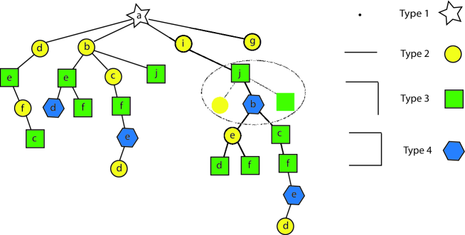
Figure 2: Assignment of the four types from matrix $\boldsymbol{N}$ defined in (7) to the self-avoiding walk tree $T_{\mathrm{saw}}$ from Figure 1. In the circled area, we also draw redundant leaves at vertex $j$ which may appear in the branching rule, but not in $T_{\mathrm{saw}}$.

See Figure 2 for an illustration of this branching matrix $\boldsymbol{N}$. One can verify that this branching matrix captures, inter alia, the self-avoiding walk trees from $\mathbb{Z}^{2}$:

Observation 2.

For any finite subgraph $G=(V,E)$ of $\mathbb{Z}^{2}$ and $v\in V$, $T_{\mathrm{saw}}(G,v)\in\mathcal{F}_{\leq\boldsymbol{N}}$.

For this branching matrix, one can check that the (DMS) condition of Theorem 7 holds with $\lambda^{*}=1.8801$, $\boldsymbol{S}=\textrm{{Diag}}(1.040,1.388,1.353,1.255)$ and $\boldsymbol{c}=(0.266037,0.100891,0.100115,0.0973861)$. Checking the DMS Condition for a given choice of parameters would have been a straightforward task, were it not for the irrationality of the coefficients $D_{jj}$. However, one can establish rigorous upper bounds for $D_{jj}$, based on concavity of the function (of $\alpha$) used in the definition of $D_{jj}$, in a suitable range of the parameters. These details will be discussed further below. As a consequence, we can conclude that Theorem 8 holds for $\boldsymbol{N}$ and $\lambda^{*}=1.8801$.

The primary reason why the branching matrix $\boldsymbol{N}$ improves beyond the tree-threshold of $\lambda<\lambda_{c}(\mathbb{T}_{4})=27/16=1.6875$ is that the average branching factor of any $T\in\mathcal{F}_{\leq\boldsymbol{N}}$ is significantly smaller than that of the regular tree of degree $4$.

To obtain a further reduction in the average branching, we observe that $\boldsymbol{N}$ did not consider the effect of occupying (or unoccupying) certain leaves as prescribed in Weitz’s construction. Starting with $T_{4}$, prune the leaves as is done in the construction of $T_{\mathrm{saw}}(\mathbb{Z}^{2})$ from Section 2.2. Denote the new tree as $T_{4}^{\prime}$. Clearly we still have that $T_{\mathrm{saw}}(\mathbb{Z}^{2})$ is a subtree of $T_{4}^{\prime}$.

Let us illustrate the difference between $T_{4}$ and the pruned tree $T_{4}^{\prime}$. We first fix an underlying order for the neighbors of each vertex. To this end, say $N>E>S>W$ and this prescribes an ordering of the neighbors of each vertex. Consider a leaf vertex $v^{\prime}$ in the tree $T_{4}$ corresponding to the vertex $v$ in $\mathbb{Z}^{2}$ and to the path $\rho$ in $\mathbb{Z}^{2}$. Since $v^{\prime}$ is a leaf vertex in $T_{4}$, $\rho$ must end with a cycle at $v$, say $WNES$. Since $v$ was exited in the West direction at the beginning of the 4-cycle, and since $W<N$, the leaf vertex $v^{\prime}$ would be labeled occupied in Weitz’s construction, thus resulting in the removal of $v^{\prime}$ and its parent in the construction of $T_{4}^{\prime}$. Note, every vertex $w^{\prime}$ in $T_{4}$ of type $WNE$ has a child $v^{\prime}$ of type $NES$, and consequently $w^{\prime}$ (and its subtree) will be removed from the tree in the pruning process to construct $T_{4}^{\prime}$. Thus, after removing vertices of type $WNE$ (and similarly, $WSE$, $SEN$ and $ENW$) from $T_{4}$, it is still the case that $T_{\mathrm{saw}}(\mathbb{Z}^{2})$ is a subtree of the resulting tree ($T_{4}^{\prime}$). This highlights why $T_{4}^{\prime}$ has a significantly smaller average branching factor than $T_{4}$.

We can define a branching matrix $\boldsymbol{M}_{2}$, with 17 types (as illustrated in Figure 3), such that $T_{4}^{\prime}\in\mathcal{F}_{\leq\boldsymbol{M}_{2}}$, and hence $T_{\mathrm{saw}}(\mathbb{Z}^{2})\in\mathcal{F}_{\leq\boldsymbol{M}_{2}}$. We can prove the DMS Condition is satisfied for $\boldsymbol{M}_{2}$ at $\lambda^{*}={2.1625}$, as we will describe shortly, which significantly improves upon our initial bound resulting from considering $T_{4}$.

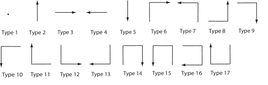
Figure 3: Shapes that the seventeen types (or labels) represent for $\boldsymbol{M}_{2}$ where $T_{4}^{\prime}\in\mathcal{F}_{\leq\boldsymbol{M}_{2}}$.

A natural direction for improved results is to consider branching matrices corresponding to avoidance of larger cycles, while also accounting for the removal of vertices prescribed by the construction of Weitz. We briefly outline such an approach for walks avoiding cycles of length at most 4, 6, and 8, respectively. Avoiding cycles of length $2i$ results in $\sum_{j\leq 2i-1}4^{j}\leq 5^{2i-1}$ types, hence the computations become increasingly difficult for larger $i$. For 8-cycles the task of finding appropriate parameters to satisfy the conditions of Theorem 7 is still feasible.

More precisely, we can define branching matrices $\boldsymbol{M}_{i}$ for $i\geq 2$, that (i) represent the structure of trees of walks avoiding cycles of length $\leq 2i$, as well as (ii) account for the removal of vertices based on children being labeled ‘occupied.’ One can extend the above construction of $\boldsymbol{M}_{2}$ for general $i>2$ by using types encoded by longer paths with length at most $2i$ and ruling out the types that either contain a cycle of length at most $2i$ or whose children end up being labeled occupied. We can make the following general observation from our construction.

Observation 3.

For any finite subgraph $G=(V,E)$ of $\mathbb{Z}^{2}$ and $v\in V$, $T_{\mathrm{saw}}(G,v)\in\mathcal{F}_{\leq\boldsymbol{M}_{i}}$ for any $i\geq 2$.

As mentioned earlier, the matrix $\boldsymbol{M}_{2}$ constructed above consists of $17$ types. An explicit description of it is shown in the Online Appendix [35], along with the associated parameters $\boldsymbol{S}$ and $\boldsymbol{c}$ for which one can check the DMS Condition for $\lambda^{*}={2.1625}$; this establishes Theorem 8 for $\boldsymbol{M}_{2}$ and $\lambda^{*}={2.1625}$.

The following table summarizes the threshold $\lambda^{*}$ we obtain for each $\boldsymbol{M}_{i}$:

Max length of Avoiding-cycles	Effect of Occupations	Number of Types	$\lambda^{*}$
4	No	4	1.8801
4	Yes	17 $(<5^{3})$	2.1625
6	Yes	132 $(<5^{5})$	2.3335
8	Yes	922 $(<5^{7})$	2.3882

Note that, one can further improve the bound on $\lambda$ by using more types for higher $i$ and hence Theorem 8 on $\mathbb{Z}^{2}$ will hold with the corresponding activity $\lambda^{*}$. For any such matrix, the verification of the DMS Condition relies on (i) ‘guessing’ appropriate values for the parameters $\boldsymbol{S}$ and $\boldsymbol{c}$ and (ii) formally verifying that DMS Condition holds for the chosen $\boldsymbol{S}$ and $\boldsymbol{c}$. In choosing desirable $\boldsymbol{S}$ and $\boldsymbol{c}$, we employed a heuristic random walk algorithm.

To verify that the DMS Condition holds for a given rational matrix $\boldsymbol{S}$ and vector $\boldsymbol{c}$ is straightforward, provided we can obtain a rational upper bound for each type $j$ for the function:

$$f_{j}(\alpha)=\frac{\left(1-\alpha\right)\left(1-\theta_{j}\left(\frac{1-\alpha}{\lambda\alpha}\right)^{1/\Delta_{j}}\right)}{s_{j}-\alpha}\,.$$

Indeed, due to the concavity of this function for $0<\theta_{j}\leq 1$, $s_{j}>51/50$ and $\lambda>27/16$, it is always possible to find a provable upper bound for $f_{j}$ in such a regime. This can be done, for example, by describing a suitable ‘envelope’ for $f_{j}$ consisting of a piecewise linear function of the form:

$$g_{j}\left(\alpha\right)=\left\{\begin{array}[c]{cc}B_{\ell}&\text{if }\alpha<\alpha_{\ell}\\ \min\{b_{\ell}\left(\alpha-\alpha_{\ell}\right)+B_{\ell},b_{u}\left(\alpha-\alpha_{u}\right)+B_{u}\}&\text{if }\alpha_{\ell}<\alpha<\alpha_{u}\\ B_{u}&\text{if }\alpha>\alpha_{u}\end{array}\right.$$

where $\alpha_{\ell},\alpha_{u}$ are points such that $b_{\ell}>f_{j}^{\prime}\left(\alpha_{\ell}\right)>0$, $b_{u}<f_{j}^{\prime}\left(\alpha_{u}\right)<0$, $B_{\ell}>f_{j}\left(\alpha_{\ell}\right)$ and $B_{u}>f_{j}\left(\alpha_{u}\right)$. It is clear for any such function that $g_{j}(\alpha)>f_{j}(\alpha)$, thus we obtain a provable upper bound for $f_{j}$ using $g_{j}$.

For every $\boldsymbol{M}_{i}$ in the above table, we provide $\boldsymbol{S}$ and $\boldsymbol{c}$, along with appropriate envelopes that lead to upper bounds $\widehat{D}_{jj}$ for the corresponding $D_{jj}$. Then we verify that the DMS Condition holds for the given values of $\lambda$ by replacing $D_{jj}$ with $\widehat{D}_{jj}$. For $i=2,3,4$ these values ($\boldsymbol{M}$, $\boldsymbol{S}$, $\boldsymbol{c}$, $\alpha_{\ell}$ and $\alpha_{u}$) are given in the Online Appendix [35].

6 Ising Model

The approach taken here for the hard-core model can also be employed to address corresponding questions in the well-studied Ising model. The Ising model, with inverse temperature parameter $\beta\geq 0$, on a finite graph $G=(V,E)$ is the model associated with the Gibbs distribution $\mu$ on $\Omega=\{-1,+1\}^{|V|}$ such that for $\sigma=[\sigma_{i}]\in\Omega$,

$$\mu(\sigma)~{}=~{}\frac{1}{Z}\exp\Bigl{(}\beta\sum_{(i,j)\in E}\sigma_{i}\sigma_{j}\Bigr{)}\,,$$

where the normalizing constant is the partition function: $Z=Z(G,\beta):=\sum_{\sigma\in\Omega}\exp\left(\beta\sum_{(i,j)\in E}\sigma_{i}\sigma_{j}\right)$. The notions of SSM, the self-avoiding walk tree representation, and branching trees defined for the hard-core model extend identically to the Ising model (or, for that matter, any other $2$-spin model). Moreover, an analog of Lemma 4 also follows easily for Ising. Then, by the use of an appropriate statistic $\varphi$, the following simpler analog of the DMS Condition can be proved for the Ising model.

Theorem 9.

Given a $t\times t$ branching matrix $M$ and $\beta^{*}>0$, suppose there exists $\boldsymbol{c}=(c_{1},\ldots,c_{t})>0$ such that

$$\tanh(\beta^{*})\boldsymbol{M}\boldsymbol{c}<\boldsymbol{c},$$ (8)

then SSM and the conclusions of Theorem 3 hold for $\boldsymbol{M}$ and all $\beta\in[0,\beta^{*}]$.

Proof.

First we note that Theorem 1 holds in general for all two spin models including the Ising model. Hence, Corollary 2 and Remark 1 are applicable to the Ising model as well. Further, observe that the proof of Theorem 3 (i.e., the implications of SSM) still hold for the Ising model. Consequently, we can prove Theorem 9 using similar notation and proof approach as was used for Theorem 7.

Given a tree $T\in\mathcal{F}_{\leq\boldsymbol{M}}$ and configuration $\boldsymbol{\rho}$, let us define again $\alpha=\alpha^{\boldsymbol{\rho}}_{r}(T,\beta)$ as the probability that the root $r$ of $T$ is minus-spinned. (Recall that in the hard-core model this was the probability that $r$ was unoccupied.) If $w_{1},\ldots,w_{k}$ are the children of $r$ and $T_{1},\ldots,T_{k}$ are the corresponding subtrees subtended at them, we let $\alpha_{i}:=\alpha^{\boldsymbol{\rho}}_{w_{i}}(T_{i},\beta)$ for $i\leq k$. For $i>k$, we define $\alpha_{i}:=1/2$. Further let $\vartheta_{i}=\frac{1-\alpha_{i}}{\alpha_{i}}$, and $\vartheta=\frac{1-\alpha}{\alpha}$. Using these notations, a straightforward recursion calculation with the partition function leads to the following:

$$\vartheta=\prod_{i=1}^{\Delta_{j}}\frac{\exp(2\beta)\vartheta_{i}+1}{\vartheta_{i}+\exp(2\beta)}\,,$$ (9)

where $j$ is the type of $r$, and $\Delta_{j}=\sum_{\ell}M_{j\ell}$.

Motivated by (9), the function $F_{j}$ (defined in Section 4 for the hard-core model) can be redefined for the Ising model as follows.

$$F_{j}(m_{1},\ldots,m_{\Delta_{j}}):=\varphi_{j}\left(\prod_{i=1}^{\Delta_{j}}\frac{\exp(2\beta)\varphi^{-1}_{j_{i}}(m_{i})+1}{\varphi^{-1}_{j_{i}}(m_{i})+\exp(2\beta)}\right),$$

where $j_{i}$ is the type of child $w_{i}$ and $\varphi_{j}$ is the statistic for a vertex of type $j$. Further, we define $m:=\varphi_{j}(\vartheta)$ and $m_{i}:=\varphi_{j_{i}}(\vartheta_{i})$. It follows from (9) that $m=F_{j}(m_{1},\ldots,m_{\Delta_{j}}).$ Then, one can prove the ‘Ising version’ of Lemma 4 with the interval $I=[\exp(-2\beta\Delta),\exp(2\beta\Delta)]$ using the same arguments as those in the proof of Lemma 4. Further, using the same arguments as in the proof of Theorem 7, with the choice of $\varphi_{j}(x):=\log(x)$, we have that

$$\frac{\partial F_{j}}{\partial m_{i}}=\frac{\vartheta_{i}\left(e^{4\beta}-1\right)}{\left(e^{2\beta}\vartheta_{i}+1\right)\left(e^{2\beta}+\vartheta_{i}\right)}\leq\tanh\left(\beta\right),$$

from which the desired condition (8) follows easily. This completes the proof of Theorem 9.

∎

Using Theorem 9 with branching matrices $\boldsymbol{M}$ analogous to those we employed in Section 5 for the hard-core model, we can prove that SSM holds for the Ising model on $\mathbb{Z}^{d}$ for all $\beta<\beta^{*}$ as detailed in the following table:

Dimension	$\beta^{*}$
2	0.392190
3	0.214247
4	0.148045
5	0.113347

In comparison, applying Weitz’s general technique to $\mathbb{Z}^{2}$ implies SSM for $\beta<.34657$.

We do not investigate the Ising model further because there are much stronger results known for this model. Onsager [24] established that $\beta_{c}(\mathbb{Z}^{2})=\log(1+\sqrt{2})\approx 0.440686$. And for general trees, Lyons [20, Theorem 2.1] established the critical point for uniqueness.

7 Acknowledgements

We are grateful to Karsten Schwan and the CERCS group at Georgia Tech for lending the support of their GPU machines so that we could conduct efficient parallel computations.

References

• [1] S. E. Alm. Upper bounds for the connective constant of self-avoiding walks. Combinatorics, Probability and Computing, 4(2):115-136, 1993.
• [2] D. S. Arnon, G. E. Collins, S. McCallum. Cylindrical Algebraic Decomposition I: The Basic Algorithm. SIAM Journal on Computing, 865-877, 1984.
• [3] R. J. Baxter, I. G. Enting and S. K. Tsang. Hard-square lattice gas. Journal of Statistical Physics, 22(4):465-489, 1980.
• [4] V. Beffara and H. Duminil-Copin. The self-dual point of the two-dimensional random cluster model is critical for $q\geq 1$. To appear in Probability Theory and Related Fields. Preprint available from the arXiv at: http://arxiv.org/abs/1006.5073
• [5] J. van den Berg and A. Ermakov. A new lower bound for the critical probability of site percolation on the square lattice. Random Structures and Algorithms, 8(3):199-212, 1996.
• [6] J. van den Berg and J. E. Steif. Percolation and the hard-core lattice gas model. Stochastic Processes and their Applications, 49(2):179–197, 1994.
• [7] G. R. Brightwell, O. Häggström, and P. Winkler. Nonmonotonic behavior in hard-core and Widom-Rowlinson models. Journal of Statistical Physics, 94(3):415–435, 1999.
• [8] F. Cesi. Quasi–factorization of the entropy and logarithmic Sobolev inequalities for Gibbs random fields. Probability Theory and Related Fields, 120(4):569–584, 2001.
• [9] R. L. Dobrushin. The problem of uniqueness of a Gibbsian random field and the problem of phase transitions. Functional Analysis and its Applications, 2(4):302-312. 1968.
• [10] R. L. Dobrushin and S. B. Shlosman. Constructive unicity criterion. In Statistical Mechanics and Dynamical Systems, J. Fritz, A. Jaffe, and D. Szasz, eds., Birkhäuser, New York, pp. 347-370, 1985.
• [11] M. E. Dyer, A. Sinclair, E. Vigoda, and D. Weitz. Mixing in time and space for lattice spin systems: A combinatorial view. Random Structures and Algorithms, 24(4):461-479, 2004.
• [12] A. Galanis, Q. Ge, D. Štefankovič, E. Vigoda, and L. Yang. Improved Inapproximability Results for Counting Independent Sets in the Hard-Core Model. Preprint, 2011. Preprint available from the arXiv at: http://arxiv.org/abs/1105.5131
• [13] D. S. Gaunt and M. E. Fisher. Hard-Sphere Lattice Gases. I. Plane-Square Lattice. Journal of Chemical Physics, 43(8):2840-2863, 1965.
• [14] H.-O. Georgii. Gibbs Measures and Phase Transitions, de Gruyter, Berlin, 1988.
• [15] L. Goldberg, R. Martin and M. Paterson. Strong Spatial Mixing for Lattice Graphs with Fewer Colours. SIAM Journal on Computing, 35(2):486-517, 2005.
• [16] C. Greenhill. The complexity of counting colourings and independent sets in sparse graphs and hypergraphs. Computational Complexity, 9(1):52–72, 2000.
• [17] M. R. Jerrum, L. G. Valiant, and V. V. Vazirani. Random generation of combinatorial structures from a uniform distribution distribution. Theoretical Computer Science, 43(2-3):169-186, 1986.
• [18] F. P. Kelly. Loss Networks. Annals of Applied Probability, 1(3):319-378, 1991.
• [19] D. A. Levin, Y. Peres, and E. L. Wilmer. Markov Chains and Mixing Times. American Mathematical Society, 2008.
• [20] R. Lyons. The Ising model and percolation on trees and tree-like graphs. Communications in Mathematical Physics, 125(2):337-353, 1989.
• [21] F. Martinelli. Lectures on Glauber dynamics for discrete spin models. Lectures on Probability Theory and Statistics (Saint-Flour, 1997), Lecture Notes in Mathematics, 1717:93-191, 1998.
• [22] F. Martinelli and E. Olivieri. Approach to equilibrium of Glauber dynamics in the one phase region. I. The attractive case. Communications in Mathematical Physics, 161(3):447-486, 1994.
• [23] F. Martinelli and E. Olivieri. Approach to equilibrium of Glauber dynamics in the one phase region. II. The general case. Communications in Mathematical Physics, 161(3):487-514, 1994.
• [24] L. Onsager. Crystal statistics. I. A two-dimensional model with an order-disorder transition. Physics Review Letters, 65(3-4):117-149, 1944.
• [25] A. Pönitz and P. Tittman. Improved upper bounds for self-avoiding walks in $\mathbb{Z}^{d}$. Electronic Journal of Combinatorics, 7(1):R21, 2000.
• [26] Z. Rácz. Phase boundary of Ising antiferromagnets near $H=H_{c}$ and $T=0$: Results from hard-core lattice gas calculations. Physical Review B, 21(9):4012-4016, 1980.
• [27] D. C. Radulescu. A computer-assisted proof of uniqueness of phase for the hard-square lattice gas model in two dimensions. Ph.D. dissertation, Rutgers University, New Brunswick, NJ, USA,1997.
• [28] D. C. Radulescu and D. F. Styer. The Dobrushin-Shlosman phase uniqueness criterion and applications to hard squares. Journal of Statistical Physics, 49(1-2):281-295, 1987.
• [29] D. Randall. Slow mixing of Glauber dynamics via topological obstructions. In Proceedings of the 17th Annual ACM-SIAM Symposium on Discrete Algorithms (SODA), 870-879, 2006.
• [30] A. Sly. Computational Transition at the Uniqueness Threshold. In Proceedings of the 51st Annual IEEE Symposium on Foundations of Computer Science (FOCS), 287-296, 2010.
• [31] D. Štefankovič, S. Vempala, and E. Vigoda. Adaptive Simulated Annealing: A Near-optimal Connection between Sampling and Counting. Journal of the ACM, 56(3):1-36, 2009.
• [32] A. Tarski. A Decision Method for Elementary Algebra and Geometry. 2nd edition, University of California Press, 1951.
• [33] L. G. Valiant. The Complexity of Enumeration and Reliability Problems. SIAM J. Computing, 8(3):410-421, 1979.
• [34] D. Weitz. Counting independent sets up to the tree threshold. In Proceedings of the 38th Annual ACM Symposium on Theory of Computing (STOC), 140–149, 2006.
• [35] Data is available from: http://www.cc.gatech.edu/$\sim$vigoda/hardcore.html
• [36] See: http://reference.wolfram.com/mathematica/tutorial/RealPolynomialSystems.html