Criticality of compact and noncompact quantum dissipative $Z_{4}$ models in $(1+1)$ dimensions

Abstract

Using large-scale Monte Carlo computations, we study two versions of a $(1+1)$D $Z_{4}$-symmetric model with ohmic bond dissipation. In one of these versions, the variables are restricted to the interval $[0,2\pi\rangle$, while the domain is unrestricted in the other version. The compact model features a completely ordered phase with a broken $Z_{4}$ symmetry and a disordered phase, separated by a critical line. The noncompact model features three phases. In addition to the two phases exhibited by the compact model, there is also an intermediate phase with isotropic quasi-long-range order. We calculate the dynamical critical exponent $z$ along the critical lines of both models to see if the compactness of the variable is relevant to the critical scaling between space and imaginary time. There appears to be no difference between the two models in that respect, and we find $z\approx 1$ for the single phase transition in the compact model as well as for both transitions in the noncompact model.

I Introduction

The standard way of introducing dissipation in a quantum mechanical system is to couple some variable describing the system to the degrees of freedom of an external environmentCaldeira and Leggett (1983). The environment is modeled as a bath of harmonic oscillators which couple linearly to the system variables. The oscillator degrees of freedom, appearing in the action to second order, may be integrated out to produce an effective theory for the composite system given in terms of the system variables.

The presence of a dissipative term introduces strongly retarded (nonlocal in time) self-interactions of the system variables. This long-range interaction in imaginary time may have serious consequences for the quantum critical behavior of the system. This effect can usually be described by a dynamical critical exponent $z$ defined by the anisotropy of the divergence of the correlation lengths at criticality, $\xi_{\tau}\sim\xi^{z}$, where $\xi$ and $\xi_{\tau}$ are the correlation lengths in space and imaginary time, respectively. An Ising spin chain with site dissipation was shown by extensive Monte Carlo simulations in Ref. Werner et al., 2005a to have $z\approx 2$. The same model, augmented to two spatial dimensions, was investigated by the present authors in Ref. Sperstad et al., 2010. The result $z=1.97(3)$ suggests that the dynamical critical exponent is independent of the number of spatial dimensions, in agreement with naive scaling arguments which make no reference to dimensionality.Hertz (1976) On the other hand, when coupling the reservoir to bond variables involving Ising spins the dissipation term was found to be irrelevant to the universality class, i.e., $z\approx 1$.Sperstad et al. (2010) In general, dissipation suppresses certain types of quantum fluctuations, though the larger value of $z$ for site dissipation signifies that bond dissipation is far less effective than site dissipation in reducing fluctuations.

Ohmic dissipation in terms of gradients or bonds is common in models describing shunted Josephson junctions or granular superconductor systems.Chakravarty et al. (1986, 1988) Here, the bonds represent the difference of the quantum phases between the superconducting grains. In this context it is well-known that the coupling of the environment to the system may affect the natural domain of the system variables.Sch n and Zaikin (1990) For Josephson junctions, this means that the domain of the phase variables reflects quantization of the charges on each superconducting grain. If the charges are quantized in units of Cooper pairs, $2e$, the domain of the quantum phase is $2\pi$-periodic. Ohmic shunting leads to an unbounded $-\infty<\theta<\infty$ domain,Sch n and Zaikin (1990) reflecting a continuous transfer of charges across the junction. We will henceforth refer to the variable defined on a restricted $2\pi$ interval as compact and the extended variable as noncompact.

Moreover, dissipation in terms of bonds has also been proposed in an effective model describing the low-energy physics of fluctuating loop currents to describe anomalous normal state properties of high-$T_{c}$ cuprates. Aji and Varma (2007, 2009) A quantum statistical mechanical model for such degrees of freedom has been derived from a microscopic three-band model of the cuprates.Børkje and Sudbø (2008) The classical part of the derived action consists in its original form of two species of Ising variables within each unit cell, coupled by a four-spin Ashkin-Teller term. This model has been proven, through large-scale Monte Carlo simulations, to support a phase transition with a non-divergent non-analyticity in the specific heat on top of an innocuous background.Grønsleth et al. (2009) The breaking of the Ising-like symmetry describes a suggested ordering of loop currents upon entering the pseudogap phase of the cuprates. Neglecting the Ashkin-Teller interaction term present in this theory, the classical model may be mapped onto a four-state clock model, with the basic variable being an angle parametrizing the four possible current loop orientations.Aji and Varma (2007); Børkje and Sudbø (2008); Grønsleth et al. (2009)

The quantum version of this model includes a kinetic energy term describing the quantum dynamics of the angle variables. Adding dissipation of angle differences as in the Caldeira-Leggett approach for Josephson junctions, the model has been reported to exhibit local quantum criticality. Local quantum criticality in this context means that the model exhibits a fluctuation spectrum which only depends on frequency, but is independent of the wave vector.Aji and Varma (2007) This essentially implies a dynamical critical exponent $z\rightarrow\infty$. A point which quite possibly is of importance in this context, is that while the starting point in Ref. Aji and Varma, 2007 is a model with two Ising-like variables, the actual dissipative quantum model discussed is one with global $U(1)$ symmetry.

While the physical picture of fluctuating configurations of current loops suggests an identification of the angles $\theta$ and $\theta+2\pi$, the presence of the clearly noncompact dissipation term makes this not entirely obvious. It is therefore the intent of this work to investigate if the restriction of the variable domain influences the dynamical critical exponent $z$, and thereby if it may have consequences for possible manifestations of local quantum criticality in similar models. Since it is still an open question exactly what the consequences are of how the variable domains are defined in dissipative quantum models, a numerical comparison of the compact and noncompact case is of general interest. We will therefore not restrict the interpretation of the model to Ising variables associated with loop currents, although the $Z_{4}$ symmetry reflecting this starting point will be maintained. Moreover, due to the long-ranged interactions in the imaginary-time direction, the Monte Carlo computations are extremely demanding. Since we are interested in a proof of principle of the importance of compactness versus noncompactness, we will in this paper limit ourselves to a $(1+1)$D model.

We will perform Monte Carlo simulations on two versions of a dissipative $Z_{4}$ model described in more detail in Sec. II, one with compact variables (i.e., a clock model) and one with noncompact variables. The simulation details are described in Sec. III, after which we present the results, first for the noncompact case in Sec. IV, then for the compact case in Sec. V.

Our main finding is that, although the critical scaling of space and imaginary time is equal for both cases, i.e., $z=1$, there is a major difference in phase structure. Whereas the compact model displays a conventional order-disorder phase transition, the noncompact model develops an intermediate phase characterized by power-law decay in spin correlations (quasi-long-range order) and a $U(1)$ symmetric distribution of the complex order parameter. The appearance of this intermediate phase is related to the fact that the kinetic energy term must be treated differently for the compact and noncompact cases, as we discuss in detail in the Appendix.

It is well established that this kind of critical phase occurs in classical 2D $Z_{q}$ clock models and $XY$ models with $Z_{q}$ anisotropy,Elitzur et al. (1979); José et al. (1977); Roomany and Wyld (1981) but only for larger values of $q$ than we are considering. It is remarkable that the noncompact model presented in this paper exhibits a critical phase with emergent $U(1)$ symmetry, when the dissipationless starting point is a pure $Z_{4}=Z_{2}\times Z_{2}$ model (i.e., a double Ising model) with the angle variables restricted to four discrete values by a hard constraint. We will discuss this in more detail in Sec. VI, after which we summarize our results in Sec. VII.

II The model

The starting point for our model is a chain of $N_{x}$ quantum rotors, or equivalently planar spins, the alignment of which is described by a set of angle variables $\{\theta_{x}\}$. Although these variables could also be denoted as the phases of the quantum rotors, we will refer to them simply as angles. Requiring that the spins satisfy $Z_{4}$ symmetry, the angles can be parametrized as $\theta=2\pi n/4$ with integer $n$, making our model similar to a four-state (or $Z_{4}$) clock model. Being quantum spins, their dynamics is described by their evolution in imaginary time $\tau$, with $N_{\tau}$ denoting the number of Trotter slices used to discretize the imaginary time dimension. The variables $\{\theta_{x,\tau}\}$ are thus defined on the vertices of a $(1+1)$D quadratic lattice of size $N_{x}\times N_{\tau}$.

In order to investigate if the restriction on the angle variable is relevant to the dynamical critical exponent $z$ or not, we will consider two variants of this model, with the complete action for both stated below for later reference. In the compact (C) case, we restrict the parametrization variable $n$ to just four values, so that the angle $\theta$ is restricted to one primary interval, corresponding to the four primary states of the four-state clock model. In the noncompact (NC) case we have no such restriction, and $n$ can take any integer values. The general form of the action is

$$S^{\mathrm{C,NC}}=S_{\tau}^{\mathrm{C,NC}}+S_{x}+S_{\mathrm{diss}},$$ (1)

where the kinetic energy for the compact and the noncompact case, respectively, is given by

$$S_{\tau}^{\mathrm{C}} =-K_{\tau}\sum_{x=1}^{N_{x}}\sum_{\tau=1}^{N_{\tau}}\cos(\theta_{x,\tau+1}-\theta_{x,\tau}),$$ (2)

$$S_{\tau}^{\mathrm{NC}} =\frac{K_{\tau}}{2}\sum_{x=1}^{N_{x}}\sum_{\tau=1}^{N_{\tau}}(\theta_{x,\tau+1}-\theta_{x,\tau})^{2}.$$ (3)

The spatial interaction defines a periodic potential

$$S_{x}=-K\sum_{x=1}^{N_{x}}\sum_{\tau=1}^{N_{\tau}}\cos(\theta_{x+1,\tau}-\theta_{x,\tau}),$$ (4)

and the dissipation term is defined according to

$$S_{\mathrm{diss}}=\frac{\alpha}{2}\sum_{x=1}^{N_{x}}\sum_{\tau\neq\tau^{\prime}}^{N_{\tau}}\left(\frac{\pi}{N_{\tau}}\right)^{2}\frac{\left(\Delta\theta_{x,\tau}-\Delta\theta_{x,\tau^{\prime}}\right)^{2}}{\sin^{2}(\frac{\pi}{N_{\tau}}|\tau-\tau^{\prime}|)}.$$ (5)

The bond variable or angle difference is written as $\Delta\theta_{x,\tau}=\theta_{x+1,\tau}-\theta_{x,\tau}$.

Note that the only apparent difference between the compact and the noncompact model is the form of the kinetic energy term. When the angles are compact the short-range temporal interaction is given by a cosine term, in contrast to noncompact angles for which a quadratic form of the kinetic term must be used. The reason for this difference can be traced to the fact that, whereas canonical conjugate variables of compact angles are discrete due to the $2\pi$ periodicity of the quantum wave functions, no such restriction applies when the angles are noncompact. From a qualitative point of view the two separate forms of the temporal interaction term is expected. Considering the imaginary time history of a single variable, it is clear that a cosine interaction in imaginary time will render the ground state of the noncompact model massively degenerate. A Trotter slice may be shifted by $2\pi$ relative to the neighboring Trotter slices without any penalty in the action. However, a quadratic interaction term in the imaginary time direction lifts this degeneracy and tends to localize the angle variables.

There is nothing new about the derivation of these different kinetic terms, but as the difference is crucial to the phase structure of our models and is also rarely discussed in the literature, we include the derivation in the Appendix. In addition, in order to simulate the compact model we also need an appropriate reinterpretation of the dissipation term. We find it natural to postpone this to Sec. V.

The action is on a form identical to the model in Sec. III in Ref. Sperstad et al., 2010 apart from the nature of the variables and the resultant treatment of the dissipation term. However, we still expect the scaling arguments presented in Ref. Sperstad et al., 2010 to be valid since no reference to the actual type of variable is used. The action in Fourier space may be written

$$S\sim(\mathbf{q}^{2}+\omega^{2}+|\omega|\mathbf{q}^{2})\theta_{q}\theta_{-q},$$ (6)

neglecting any prefactors. Taking the limit $\mathbf{q}\rightarrow 0$, $\omega\rightarrow 0$ we anticipate that the term $\sim|\omega|\mathbf{q}^{2}$ describing the dissipation is subdominant for all positive $z$. Accordingly, we expect at least naively that $z=1$ for both compact and noncompact variables. This will be investigated in detail in our simulations, and we make no assumption of the veracity of naive scaling applied to this problem.

III Details of the Monte Carlo computations

When expanding the dissipative term, it becomes clear that it contributes both to ferromagnetic and antiferromagnetic long range interactions. This renders the system intractable to the Luijten-Bl teLuijten and Blöte (1995) extension of the Wolff cluster algorithmWolff (1989) which has been used with great success in systems with noncompeting interactions. Also, for the case of noncompact variables there does not exist a straightforward way of defining (pseudo)spin projections, a necessary point for the Wolff embedding technique.Wolff (1989) Considerable progress has been made in constructing new effective algorithms for long range interacting systems with extended variables.Werner and Troyer (2005a); Werner et al. (2005b); Werner and Troyer (2005b) However, these algorithms are presently restricted to $(0+1)$D systems, and do not seem to generalize easily to $N_{x}>1$.Werner et al. (2005b) Furthermore, the basic degrees of freedom in these algorithms are the phase differences between two superconducting grains in an array of Josephson junctions. Our aim is to investigate the ordering of the phases themselves. Hence, the existing non-local algorithms may not be utilized. In the Monte Carlo simulations, we have therefore used a parallel tempering algorithmHukushima and Nemoto (1996); Katzgraber (2009) in which several systems (typically 16 or 32) are simulated simultaneously at different coupling strengths.

A Monte Carlo sweep corresponds to proposing a local update by the Metropolis-Hastings algorithm for every grid point in the system in a sequential way. For the case of noncompact variables the proposed new angles are generated by randomly choosing to increase or decrease the value, then propagating the value by randomly choosing the increment on the interval $\{\frac{\pi}{2},\pi,\frac{3\pi}{2},2\pi\}$. In the case of compact variables, a new angle value in the primary interval is randomly chosen. After a fixed number of Monte Carlo sweeps (typically $3-10$) a parallel tempering move is made. In this move, a swap of configurations between two neighboring coupling values is proposed, and the swap is accepted with probability $\Xi_{PT}$ given by

$$\Xi_{PT}=\begin{cases}1&\mathrm{if}\ \Delta<0,\\ \mathrm{e}^{-\Delta}&\mathrm{if}\ \Delta\geq 0.\end{cases}$$ (7)

Here, $\Delta=\kappa^{\prime}(\bar{S}[X;\kappa^{\prime}]-\bar{S}[X^{\prime};\kappa^{\prime}])-\kappa(\bar{S}[X;\kappa]-\bar{S}[X^{\prime};\kappa])$, where $\kappa$ is the coupling value varied, representing in our case $K$ or $\alpha$, and $X$ represents the angle configuration. $\bar{S}$ indicates the term of the action proportional with the coupling parameter $\kappa$.

All Monte Carlo simulations were initiated with a random configuration. Depending on system sizes various numbers of sweeps were performed for each coupling value. For the phase transition separating the disordered state from the critical phase in the noncompact model $5-10\times 10^{6}$ sweeps were made. Also, $1-5\times 10^{5}$ sweeps at each coupling value were discarded for equilibration. For the compact model and the second transition of the noncompact model as much as $30\times 10^{6}$ sweeps where performed and typically $5\times 10^{5}$ sweeps discarded.

The Mersenne-TwisterMatsumoto and Nishimura (1998) random number generator was used in all simulations and the random number generator on each CPU was independently seeded. It was confirmed that other random number generators yielded consistent results. We also make use of the Ferrenberg-Swendsen reweighting technique,Ferrenberg and Swendsen (1989) which enables us to continuously vary the coupling parameter after the simulations have been performed.

IV Results: Noncompact model

In this section we consider the noncompact version of the dissipative $Z_{4}$ model. Using Eqs. (3), (4) and (5) we have the following action,

$$S^{\mathrm{NC}}=S_{\tau}^{\mathrm{NC}}+S_{x}+S_{\mathrm{diss}}.$$ (8)

In contrast to the compact model, the angle variables are in this case not restricted to the primary interval. The variables are straightforwardly generalized to take the values $\theta=2\pi n/4$, where $n=0,\pm 1,\pm 2,\dots$. We seek to fix $K$ and $K_{\tau}$ and investigate how the system behaves under the influence of increasing dissipation strength controlled by the dimensionless parameter $\alpha$.

The kinetic coupling strength has been fixed to $K_{\tau}=0.4$ for computational reasons, as this ensures that the simulations will be performed at convenient values of $N_{x}$ and $N_{\tau}$. We have performed simulations at four different spatial coupling constants $K=$ 0.4, 0.5, 0.6 and 0.75. These choices are also made for computational convenience, as the limit of vanishing dissipation as well as the limit $K\to 0$ are both very computationally demanding. For all coupling values there is a disordered phase at low values of the dissipation strength. In this phase the noncompact angles exhibit wild fluctuations and consequently $\langle\mathrm{e}^{\mathrm{i}\theta_{x,\tau}}\rangle=0$. However, we also have $\langle\mathrm{e}^{\mathrm{i}\Delta\theta_{x,\tau}}\rangle\neq 0$ in this phase, a trivial consequence of the cosine potential acting as an external field on the bond variables. The bond variables occasionally drift from one minimum of the extended cosine potential to another. As the dissipation strength is increased, fluctuations in these variables are suppressed, and the system features two consecutive phase transitions separated by a critical phase. This intermediate phase is characterized by power-law decay of spatiotemporal spin correlations on the form

$$g(\mu)=\langle\mathrm{e}^{\mathrm{i}(\theta_{\mu}-\theta_{0})}\rangle,\hskip 8.53581pt\mu\in(x,\tau).$$ (9)

The correlation functions for both spatial and imaginary time direction are shown in Fig. 1 for two different dissipation strengths both within the the critical phase.

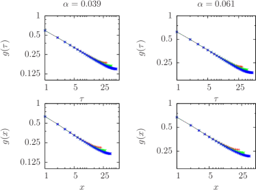
Figure 1: (Color online) Correlation functions, Eq. (9), at two values of the dissipation strength $\alpha$ within the critical phase for spatial coupling $K=0.75$. System sizes are $N_{x}=44,57,74$, with optimal choices of $N_{\tau}$ at $\alpha_{c}^{(1)}$, see text. Top row: Correlation functions for the temporal direction. Bottom row: Correlation functions for the spatial direction.

A very similar critical phase, as well as phase transitions associated with it, has recently enjoyed increased interest in various versions of classical clock models.Lapilli et al. (2006); Baek and Minnhagen (2010); Baek et al. (2009) We will proceed under the assumption that a similar picture is valid in our case. Indeed, simulations performed on a classical 2D six-state clock give qualitatively very similar results for all observables considered below, which supports the supposition that these two phenomena are related.

Considering the complex order parameter of the system,

$$m=\frac{1}{N_{x}N_{\tau}}\sum_{x,\tau}\mathrm{e}^{\mathrm{i}\theta_{x,\tau}}=|m|\mathrm{e}^{\mathrm{i}\phi},$$ (10)

the intermediate critical phase can be identified by observing the distribution of $m$ in the complex plane. Baek et al. (2009) In the disordered phase, the order parameter is a Gaussian peak centered at the origin. In the intermediate phase, quasi-long-range order develops in the complex order parameter, and so $|m|$ acquires a nonzero value as a finite-size effect. The order parameter is, however, free to rotate in the $\phi$ direction. This can be described as the vanishing of the excitation gap naively expected for discrete $Z_{q}$ models, or equivalently as an emergent $U(1)$ symmetry.Lou et al. (2007) This symmetry is broken at a larger value of the dissipation strength, when true long-range order is established when the magnetization selects one of the four well-defined directions in the complex plane originating with the underlying $Z_{4}$ symmetry. Typical distributions of the complex order parameter in the three phases is shown in Fig. 2.

(a) Two dimensional Gaussian distribution of the order parameter in the complex plane corresponding to the disordered phase with $\alpha=0.0<\alpha_{c}^{(1)}$.

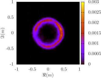
(b) Intermediate critical phase exhibiting a finite-size-induced non-vanishing $|m|$ that rotates in the $\phi$ direction. The critical phase exists in a finite interval of dissipation strengths $\alpha_{c}^{(1)}<\alpha=0.04<\alpha_{c}^{(2)}$. The remaining anisotropy is attributed to insufficient sampling. Hove and Sudbø (2003)

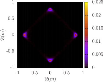
(c) The rotational symmetry of the intermediate critical phase is broken and long-range order is established as the order parameter relaxes into one of the four directions in the complex plane. The long-range ordered phase corresponds to the strong dissipation limit, $\alpha=0.18>\alpha_{c}^{(2)}$.

Figure 2: (Color online) Evolution of the complex order parameter when dissipation strength $\alpha$ is increased for $K=0.75$ and system size $N_{x}=74$, $N_{\tau}=103$ which corresponds to a near optimal aspect ratio at the phase transition at $\alpha\approx\alpha_{c}^{(1)}$. The color scale indicates relative density of the distribution.

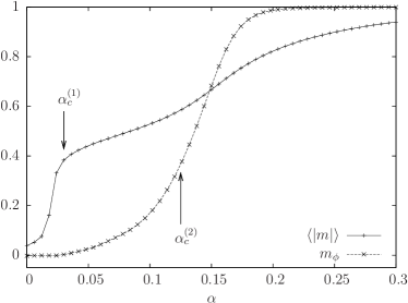
Figure 3: The order parameter $\langle|m|\rangle$ and the anisotropy measure $m_{\phi}$ of the noncompact $Z_{4}$ model with $K=0.75$ and system size $N_{x}=74$, $N_{\tau}=103\approx N_{\tau}^{\ast}$. This size represents a near optimal aspect ratio at $\alpha\approx\alpha_{c}^{(1)}$. The two phase transitions are indicated by arrows, note that the intermediate critical phase $\alpha_{c}^{(1)}<\alpha<\alpha_{c}^{(2)}$ features a rotationally symmetric order parameter distribution.

Although not presented here, we have also confirmed that the susceptibility of the order parameter diverges over a finite interval of dissipation strengths, also a clear evidence of a critical phase.

The phase transition between the disordered state and the intermediate critical phase at dissipation strength $\alpha=\alpha_{c}^{(1)}$ is detected by the Binder cumulant $g=1-Q/3$, where

$$Q=\frac{\langle|m|^{4}\rangle}{\langle|m|^{2}\rangle^{2}}.$$ (11)

The brackets indicate ensemble averaging. The scaling at criticality of the Binder cumulant for anisotropic systems is given in terms of two independent scaling variables,Werner et al. (2005a)

$$g(N_{x},N_{\tau})=\mathcal{G}\left(\frac{N_{x}}{\xi},\frac{N_{\tau}}{\xi^{z}}\right).$$ (12)

At a critical point the correlation length $\xi$ diverges, and one should be able to observe data collapse of the Binder cumulant as a function of $N_{\tau}/N_{x}^{z}$ for the correct value of $z$. The value of $g(N_{x},N_{\tau})$ is independent of $N_{x}$ at the critical coupling, this may be used to align the plots of $g$ as a function of $N_{\tau}$ horizontally. The exponent $z$ can then be found by optimal collapse of data onto a universal curve. The cumulant curves have a maximum at $N_{\tau}=N_{\tau}^{\ast}$. At this temporal size, the system appears as isotropic as it can be, the anisotropic interactions taken into account. See Ref. Sperstad et al., 2010 for a thorough discussion of this finite-size analysis.

In the intermediate phase, the system is critical over a finite interval of dissipation strengths. According to the scaling Eq. (12), curves of the Binder cumulant for increasing system sizes will therefore merge in this interval for $N_{x}\rightarrow\infty$.Loison (1999) For systems of finite sizes as considered here, the curves will however intersect close to the transition instead, and we find $\alpha_{c}^{(1)}$ by inspecting the convergence of the crossing points. As discussed in Ref.  Sperstad et al., 2010, the functional form of this convergence is unknown in our case (cf. also Sec. VI and Ref.  Loison, 1999), and all we can do is to report our best estimate for the $N_{x}\rightarrow\infty$ transition point. The uncertainty estimated accordingly is not insignificant, but the effective critical exponent $z$ is found to not be very sensitive to this error in $\alpha_{c}$.

By further increasing the dissipation strength, the rotational symmetry of the global order parameter is broken at $\alpha=\alpha_{c}^{(2)}$. The Binder cumulant given by Eq. (11) will not pick up this transition because $|m|$ does not contain any information on the angular direction of the global magnetization. Therefore, we consider an alternative magnetization measureLou et al. (2007); Baek et al. (2009)

$$m_{\phi}=\langle\cos(4\phi)\rangle,$$ (13)

where $\phi$ is the global phase as indicated by Eq. (10). This anisotropy measure vanishes when $\phi$ is evenly distributed and tends toward unity when the excitation gap opens and $\phi$ gets localized. We show in Fig. 3 both order parameters for the system $N_{x}=74,N_{\tau}=103$ as a function of $\alpha$. This $N_{\tau}$ corresponds to the nearest integer $N_{\tau}^{\ast}$ at $\alpha\approx\alpha_{c}^{(1)}$. Actually, the optimal $N_{\tau}$ decreases with increasing $\alpha$, so the given system size does not represent an optimally chosen aspect ratio for other dissipation strengths. The rotational symmetry of the complex order parameter is clearly seen to be broken at a higher dissipation strength than the onset of the intermediate critical phase.

Because $\phi$ measures a global rotation of the order parameter, extremely long simulations is needed to explore the $\phi$ space with a local update algorithm. This limits the efficiency of constructing a Binder cumulant from $m_{\phi}$ and extracting $\alpha_{c}^{(2)}$ from a universal point because this would involve calculating moments of a already statistically compromised ensemble. To alleviate these difficulties, we instead make a scaling ansatz for the anisotropy measure itself,

$$m_{\phi}=\mathcal{M}_{\phi}\left(\frac{N_{x}}{\xi},\frac{N_{\tau}}{\xi^{z}}\right),$$ (14)

based on the fact that the naive scaling dimension of this magnetization measure is zero. Near criticality, we expect $m_{\phi}$ to scale with system size in the same way as the Binder cumulant Eq. (12). Hence, we may calculate a dynamical critical exponent for this transition by exactly the same procedure as in Sec. V and Ref. Sperstad et al., 2010. Again we expect a merging of $m_{\phi}$ curves as $\alpha\rightarrow\alpha_{c}^{(2)}$ from above in the limit of large $N_{x}$, but for the present system sizes we use the crossing points of $m_{\phi}$ curves to estimate $\alpha_{c}^{(2)}$. In Fig. 4, we plot the resulting phase diagram in the $\alpha-K$ plane. The intermediate phase is evidently very wide also when compared to the uncertainty assigned to the transition line, and we feel confident that it is a genuine phase and not merely an effect of the admittedly moderate finite system sizes we are restricted to.

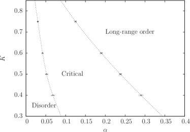
Figure 4: Phase diagram for the noncompact model, Eq. (8) with $K_{\tau}=0.4$. The dotted lines are guides to the eye. For fixed $K$ the model features two consecutive phase transitions surrounding the intermediate critical phase (with quasi-long-range order). The simulation results (symbols along the dotted lines) are restricted to a region in coupling space amenable to simulations.

We extract the dynamical critical exponent $z$ along both of the critical lines $\alpha_{c}^{(1)}$ and $\alpha_{c}^{(2)}$ for all spatial coupling strengths. The data collapse of the Binder cumulant $g$ at $K=0.75$ and $\alpha=0.030\approx\alpha_{c}^{(1)}$ is shown in Fig. 5. Increasing the dissipation strength further brings the system to the second phase transition at $\alpha=0.125\approx\alpha_{c}^{(2)}$, the collapse of $m_{\phi}$ at this point is shown in Fig. 6.

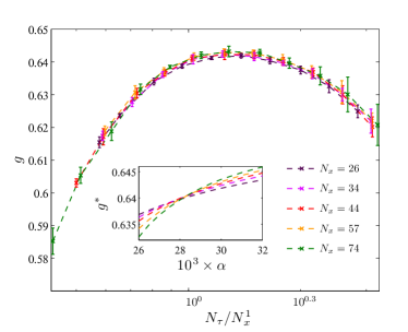
Figure 5: (Color online) Data collapse of the Binder cumulant, $g=1-Q/3$, with $Q$ given by Eq. (11), for the noncompact $Z_{4}$ model at $K=0.75$ and $\alpha=0.030\approx\alpha^{(1)}_{c}$ with $z^{(1)}=1$. Inset: Intersection of the Binder cumulant as a function of dissipation strength.

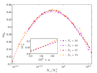
Figure 6: (Color online) Data collapse of the anisotropy measure $m_{\phi}$, Eq. (13), for the noncompact $Z_{4}$ model at $K=0.75$ and $\alpha=0.125\approx\alpha_{c}^{(2)}$ with $z^{(2)}=1$. The actual uncertainties are probably larger than indicated by the error bars for reasons discussed in the text. Inset: Intersection of the anisotropy measure as a function of dissipation strength.

In Table 1, we present the numerical estimates of the dynamical critical exponent. The values of $z$ are obtained using the scaling relation $N_{\tau}^{\ast}=aN_{x}^{z}$, with uncertainties based on a bootstrap analysis. These uncertainties also include the uncertainty in $\alpha_{c}$. Within the accuracy of the simulations, the value of the critical exponent is $z=1$ for all the coupling values at both phase transitions (although precise results are harder to obtain for the second). This is in accordance with the scaling argument presented in Sec. II.

Table 1: Numerical estimates for critical coupling and critical exponents $z^{(1),(2)}$ for the two phase transitions $\alpha_{c}^{(1),(2)}$ of the noncompact model.

$K$	$\alpha_{c}^{(1)}$	$z^{(1)}$	$\alpha_{c}^{(2)}$	$z^{(2)}$
0.75	0.030(2)	0.99(1)	0.125(2)	1.01(2)
0.6	0.042(2)	0.99(2)	0.190(3)	0.96(3)
0.5	0.053(2)	1.02(2)	0.238(3)	0.97(3)
0.4	0.068(4)	0.97(3)	0.287(5)	0.99(4)

V Results: Compact model

We now turn to the compact version of the dissipative $Z_{4}$ model,

$$S^{\mathrm{C}}=S_{\tau}^{\mathrm{C}}+S_{x}+S_{\mathrm{diss}},$$ (15)

where the three terms are given by Eqs. (2), (4) and (5), respectively. Note that we now use a kinetic term $S_{\tau}^{\mathrm{C}}$ having the same cosine-form as the spatial interaction term $S_{x}$. Regarding the use of the same dissipation term $S_{\mathrm{diss}}$ as in the noncompact case, one may argue that adding a Caldeira-Leggett term for the angle differences $\Delta\theta$ is a rather artificial way to model dissipation for a compact clock model in the first place, since its variance under $2\pi$ translations of $\theta$ implicitly assumes noncompact variables. However, adding exactly such a dissipation term is crucial for the demonstration of local quantum criticality in a similar $Z_{4}$ modelAji and Varma (2007) that is not obviously noncompact. Therefore, our motivation for the comparative study in the present section of a compactified version of the action (8) is to investigate whether an equivalent dissipation term for compact variables gives the model the same critical properties as reported for noncompact variables in the previous section, and thus whether the compactness of the variables as such is essential. Constructing an appropriate compactified version of the dissipative model does, however, require a reinterpretation of the variables in the Caldeira-Leggett term, so we will begin with a careful discussion of how we should treat this term in our simulations.

We first impose the following restriction on the interpretation of the compactified dissipation term: The term as a whole should be invariant under translations $\theta\rightarrow\theta+2\pi$, since these two states are indistinguishable. As a corollary, any configurations that are physically indistinguishable when the angles are restricted to four values $\theta\in\{-\pi,-\pi/2,0,\pi/2\}$ (or any equivalent parametrization) should give the same contribution to the dissipation term. Consequently, we cannot simply simulate the model with the dissipation term (5) as it stands, because the angle differences $\Delta\theta_{x,\tau}$ now only make physical sense modulo $2\pi$. We therefore have to bring $\Delta\theta_{x,\tau}$ back to the primary interval $[-\pi,\pi\rangle$, as is well known for phase differences in superconducting systems without dissipation and other realizations of the (compact) $XY$ model. Furthermore, we also choose to do the same for the difference between the two (compactified) $\Delta\theta_{x,\tau}$ terms in Eq. (5), as the alternative would result in different Boltzmann factors being associated with physically equivalent situations. Our procedure then is equivalent to requiring that the entire difference $\Delta\theta_{x,\tau}-\Delta\theta_{x,\tau^{\prime}}$ should be restricted to the primary interval $[-\pi,\pi\rangle$, i.e., treating the dissipation term as a $2\pi$-periodic function.

The details of the Monte Carlo simulations are described in III also for the compact model. The only difference that may be of any consequence is that we found it more convenient to vary the spatial coupling while fixing the dissipation strength in this case, but we have checked that the direction in coupling space taken by the simulations has no impact on the result.

The dissipationless ($\alpha=0$) four-state clock model is completely isomorphic to the Ising model with interaction $K/2$. Thus, we may employ the criterion $\sinh(K_{c})\sinh(K_{\tau})=1$ in order to calculate $K_{c}$ for a fixed value of $K_{\tau}$. The temporal coupling parameter is fixed at $K_{\tau}=-\ln{(\tanh{\frac{1}{2}})}\approx 0.7719$ such that $K_{c}=1$ when the dissipation is tuned to zero.

The most striking difference we found when compactifying the angles is that the intermediate phase with quasi-long-range order vanishes. This means that one has only a single disorder-order phase transition, as is the result one would usually expect for any model with $Z_{4}$ symmetry. We have verified that the $Z_{4}$ symmetry and the apparent $U(1)$ symmetry of the complex order parameter (in the disordered phase) are spontaneously broken simultaneously at a single critical point. This is found by observing that the inflection points of magnetization curves for $m$ and $m_{\phi}$ coincide asymptotically, in contrast to the curves shown in Fig. 3 for the noncompact case.

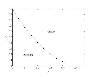
Figure 7: Phase diagram for the compact model of Eq. (15) with $K_{\tau}=-\ln{(\tanh{\frac{1}{2}})}$, the dotted line indicating a critical line separating the disordered phase from a phase with long-range order. The line is not drawn beyond $\alpha=0.4$ because of increasing uncertainties.

The phase diagram for the compact $Z_{4}$ model with bond dissipation is shown in Fig. 7. It differs considerably from that of its noncompact counterpart, not only in the evident absence of any intermediate critical phase, but also in that the limit $\alpha\rightarrow 0$ is well-behaved. Here, the model is reduced to two uncoupled 2D Ising models, for which exact results are known and simulations are straightforward. In the limit of $K\rightarrow 0$ the simulations are on the other hand very difficult for the same reasons as those investigated by us in a similar model in Ref. Sperstad et al., 2010. Therefore, we have not strived to extend the phase diagram all the way down to the $\alpha$ axis in this work. Due to the qualitative difference in the kinetic terms for the compact and noncompact model, it is not possible to make quantitative comparison between the position of the phase transition line in Fig. 7 and the two phase transition lines in Fig. 4.

Turning next to the nature of the critical line in the phase diagram, we show in Fig. 8 and Table 2 results for the three points along the line for which we made the most effort to extract the dynamical critical exponent. These points are chosen so that the relative influence of the dissipation term should be qualitatively comparable with that for the points $(\alpha_{c}^{(1)},K)$ chosen for the first transition of the noncompact model. As for the noncompact model here and the Ising model with bond dissipation studied in Ref. Sperstad et al., 2010, there is no significant variation in the dynamical critical exponent from the expected value $z=1$, although the tendency to greater finite-size effects for increasing $\alpha$ remains for both the compact and the noncompact model.

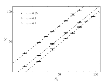
Figure 8: Finite-size analysis of the maximum $N_{\tau}^{\ast}$ of the cumulant curves as a function of spatial system size $N_{x}$ used to obtain the dynamical critical exponent $z$ for the compact model. The dashed lines show the power-law fits, cf. Table 2 for the results.

Table 2: Critical coupling $K_{c}$ and dynamical critical exponent $z$ for different values of the dissipation strength $\alpha$ for the compact model.

$\alpha$	$K_{c}$	$z$
0.05	0.8303(4)	1.02(2)
0.1	0.6753(7)	0.99(2)
0.2	0.414(2)	0.99(2)

VI Discussion

The models discussed in this paper are in some sense generalizations of the Ising spin system with bond dissipation discussed in Ref. Sperstad et al., 2010. For the compact $Z_{4}$ model the modifications come from the increase of the number of states from $q=2$ to $q=4$, while one for the noncompact model adds an additional extension of the configuration space. The phase diagram for the compact model is very much like that observed for the dissipative Ising model,Sperstad et al. (2010) both featuring a single order-disorder phase transition line. The noncompact model on the other hand exhibits much richer physics in the sense that it presents, for fixed $K$ and $K_{\tau}$, two phase transitions surrounding an intermediate critical phase with power-law decaying spin correlations and emergent $U(1)$ symmetry. The most pressing question then pertains to the occurrence of this phase: Why is the discrete structure of the angle variables rendered irrelevant in a region of parameter space for our $Z_{4}$ model, when such behavior is previously known to occur only in $Z_{q}$ models with $q>4$? Even our compactified model differs from a pure $Z_{4}=Z_{2}\times Z_{2}$ clock model, since the dissipation term couples the two underlying $Z_{2}$ models in a nontrivial way. Such models can no longer be expected a priori to behave as an Ising model, and there is in principle no reason why they may not even present intermediate phases. The absence of such a phase in our compact model does however indicate that we must turn to the other obvious difference between our model and a $Z_{4}$ clock model, namely that the variables in our noncompact model are free to drift outside the primary interval. Somehow, this added degree of freedom is enough to close the excitation gap.

As observed in Fig. 2(b), the underlying $Z_{4}$ symmetry stemming from the discreteness of the variables is irrelevant in the intermediate phase. Consequently, the system displays an effective continuous symmetry. Since $z=1$, the effective long-wavelength low-energy propagator is on a Gaussian form $1/(\omega^{2}+q^{2})$. In addition, the system is effectively two dimensional due to $z=1$. In two dimensions, Gaussian fluctuations are sufficient to induce a critical phase given a continuous symmetry. This is analogous to the mechanism producing a critical phase in the classical 2D $XY$ model with an $Z_{q>4}$ anisotropyJosé et al. (1977) [soft constraint with underlying $U(1)$ symmetry], and also for classical $Z_{q>4}$ clock modelsElitzur et al. (1979) (hard constraint). The difference in our case is that the underlying symmetry is $Z_{q=4}$.

To comment further on the origin of the critical phase, it appears that the quadratic form of the kinetic energy in the problem is essential for observing it. This quadratic short-range interaction term in imaginary time facilitates Gaussian fluctuations. Were we to use a cosine-like form of this term for noncompact variables (as one does for compact variables), this intermediate phase would not be found. The kinetic energy term is bounded from below, but not from above. Upon entering the intermediate phase from the ordered side, this term tends to suppress strong $\theta$ fluctuations, much more so than a kinetic term which is bounded from below and above, such as a cosine-like term. Only at even lower values of the dissipation are the excitation energies of larger $\theta$ fluctuations so low that wild $\theta$ fluctuations are possible due to the boundedness of the spatial coupling. At this point, the system disorders completely. If the quadratic kinetic energy term is replaced by a cosine-like term, wild $\theta$ fluctuations are facilitated precisely at the critical point where the $Z_{4}$-symmetry becomes irrelevant, and the system disorders directly from the $Z_{4}$-ordered state. Hence, for a compact model there will only be one phase transition separating the $Z_{4}$-ordered state from the completely disordered phase.

We now comment on the critical scaling between space and imaginary time in the models we have studied. For the compact case one has the conventional case of a critical line along which the correlation length diverges as $\xi\sim|K-K_{c}|^{-\nu}$ in space and $\xi_{\tau}\sim|K-K_{c}|^{-z\nu}$ in imaginary time, with $z$ appearing to remain equal to unity along the line. This picture is no longer valid in the noncompact case, as $\xi$ and $\xi_{\tau}$ are formally infinite in the entire intermediate critical phase, and $z$ can not be defined from the anisotropy of their divergence in this region. Furthermore, supposing that the intermediate phase shares qualities with the corresponding phase in classical $Z_{q>4}$ models, the correlation lengths can be expected to diverge exponentially as this critical phase is approached from either side as for the Kosterlitz-Thouless (KT) transition, and not as a power law as for conventional critical points. However, as long as the correlation length does diverge, and this divergence is exponential both in space and imaginary time, the dynamical critical exponent is still well defined through $\xi_{\tau}\sim\xi^{z}$. Therefore, our finite size analysis is valid as $\alpha\rightarrow{\alpha_{c}^{(1)}}^{-}$ and $\alpha\rightarrow{\alpha_{c}^{(2)}}^{+}$ irrespective of whether these points turns out to possess KT criticality or not. At both phase transitions we have $z=1$, signaling equally strong divergence of correlation lengths in space and imaginary time.

To infer from simulations on finite systems that the correlation length in fact diverges exponentially is exceedingly difficult,Luijten and Meßingfeld (2001); Itakura (2001); Loison (1999) and we have not attempted to determine the exact nature of the phase transitions, but leave this an open question. The phase transitions (one or both) may be in the KT universality class, or it may belong to a class of related topological phase transitions.Baek and Minnhagen (2010) This identification of the exact universality class is controversial even for classical clock models.Lapilli et al. (2006); Hwang (2009); Baek et al. (2010)

If we generalize the noncompact action in Sec. IV by redefining the phase space such that the variable can take on all real values, Eq. (8) may represent the action for a one-dimensional array of Josephson junctions.Chakravarty et al. (1986, 1988) Recent theoretical work Tewari et al. (2005, 2006) report that such systems may display local quantum criticality, in the sense that the spatial coupling renormalizes to zero at the quantum phase transition so that the behavior is essentially $(0+1)$ dimensional. This suggests that local quantum criticality need not be restricted to $(2+1)$D models such as the one presented in Ref.  Aji and Varma, 2007, but that similar unconventional criticality may be found in $(1+1)$D as well. Although it should be remembered that our $(1+1)$D model has discrete angle variables, our simulations do not show any traces of local critical behavior, in the sense that the scaling of Binder cumulants do not give $z\gg 1$.

Strictly speaking, the dynamical critical exponent is not well defined inside the intermediate phase, and the isotropic behavior is instead maintained by the decay exponents for the power-law spin correlation functions in space and time being equal. Nevertheless, for finite $N_{x}$ one may still assume the scaling relation $N_{\tau}^{\ast}=aN_{x}^{z}$ and use the ordinary procedure to extract the (effective) exponent $z$ as long as the system is critical, which yields $z\approx 1$ in the entire intermediate phase. We may then inspect how the nonuniversal prefactor $a$ changes as a reflection of the anisotropy of the interaction in time and space. In the noncompact model it is possible to investigate the development of $a$ at constant $K_{\tau}/K$ and varying $\alpha$ without leaving the critical region. We find that $a$ decreases for increasing $\alpha$, indicating that the dissipation term contributes to making the temporal dimension less ordered than the spatial one. This is also in contrast with a tendency toward $(0+1)$D behavior when increasing the dissipation strength, as suggested in the models mentioned above.

VII Conclusions

We have performed Monte Carlo simulations on two distinct $Z_{4}$-symmetric dissipative lattice models. In one model the phase variables are only defined on the interval $[0,2\pi\rangle$, while the other model has no restrictions on the variables. The different domains of the variables have implications for the short range interaction term in imaginary time, which again leads to essential differences in the behavior of the two models. The compact model features only one phase transition in which the $Z_{4}$ symmetry is spontaneously broken. On the other hand, the noncompact model displays three phases, namely a disordered phase with exponentially decaying spin correlations, an intermediate critical phase with quasi-long-range order, and finally a long-range ordered phase.

Along the phase-transition line of the compact model, we find the dynamic critical exponent $z=1$, independent of the dissipation strength. In the noncompact model, we find the value $z=1$ for both phase transitions and the power-law decay exponents for space and imaginary time are equal in the entire phase exhibiting quasi-long-range order.

We have shown that the issue of compactness versus noncompactness of the fundamental variables of the $Z_{4}$ models have important ramifications for their long-distance, low-energy physics.

Appendix A Quantum-to-classical mapping for compact and noncompact variables

In this appendix we will outline the quantum-to-classical mapping for a quantum rotor model and show how the kinetic term in the resulting classical model depends on whether the variables are interpreted as compact or noncompact. We will first reproduce the derivation as given in Refs.  Wallin et al., 1994; Sondhi et al., 1997 for the case of compact variables, after which we will generalize and reinterpret it for the noncompact case. Although there is nothing novel about this derivation, the form of the kinetic term often seems to be taken for granted in the literature, and a correct interpretation of the classical action in the noncompact case is crucial for our results. As a starting point we take the (dissipationless) Hamiltonian $H_{0}=T+U$ for a spatially extended system of particles, each moving on a ring. The kinetic energy of the rotors is given by

$$T=-\frac{1}{2I}\sum_{x}\frac{\partial^{2}}{\partial\theta_{x}^{2}},$$ (16)

where $I$ is some inertia parameter. The (periodic) potential energy is given by Josephson-like coupling of the rotors,

$$U=-K\sum_{x}\cos(\hat{\theta}_{x+1}-\hat{\theta}_{x}),$$ (17)

with $K$ being the coupling strength. Here we have used the angle representation where we for simplicity let $\theta$ be a continuous variable, and $\hat{\theta}$ is the corresponding operator. Characteristic of a rotor model is the invariance of the system upon translations of the angle $\theta\rightarrow\theta+2\pi$. The eigenfunctions describing the system should therefore be $2\pi$-periodic, a requirement which immediately yields discretized angular momenta and energy levels.

The partition function of the rotor system may be given by

$$\mathcal{Z}=\mathrm{Tr}\left(\mathrm{e}^{-\beta(T+U)}\right).$$ (18)

We let $k_{B}=1$ such that $\beta$ equals inverse temperature. The trace may be evaluated by introducing a path integral over $M$ time slices between $\tau=0$ and $\tau=\beta$, with the width of the time slices given by $\Delta\tau=\beta/M$. For every time step indexed by $\tau$, we insert a complete set of states,

$$\mathcal{Z}\approx\lim_{M\to\infty}\int\mathcal{D}\theta\prod_{\tau=0}^{M-1}\langle\theta(\tau+1)|\mathrm{e}^{-\Delta\tau T}\mathrm{e}^{-\Delta\tau U}|\theta(\tau)\rangle.$$ (19)

Here, $|\theta(\tau)\rangle$ is an angular eigenstate of all rotors with Trotter index $\tau$. Since $|\theta(\tau)\rangle$ is an eigenstate of $\hat{\theta}$ we get

$$\mathrm{e}^{-\Delta\tau U}|\theta(\tau)\rangle=|\theta(\tau)\rangle\mathrm{e}^{K\cos(\theta_{x+1,\tau}-\theta_{x,\tau})}.$$ (20)

A general matrix element describing the kinetic energy is given by

$$T_{x,\tau}=\langle\theta_{x}(\tau+1)|\mathrm{e}^{-\Delta\tau T}|\theta_{x}(\tau)\rangle.$$ (21)

Next, for each $\tau$ we insert a complete set of eigenstates of the kinetic energy $|n_{x}(\tau)\rangle$. Because $\theta$ and $n$ are conjugate variables, we have the identity $\langle n_{x}(\tau)|\theta_{x}(\tau)\rangle=\exp{[{-\mathrm{i}n_{x,\tau}\theta_{x,\tau}}]}$. Inserting this, we get the general form of the matrix element for the kinetic energy

$$T_{x,\tau}=\sum_{n_{x,\tau}} \mathrm{e}^{\mathrm{i}n_{x,\tau}\theta_{x,\tau+1}}\mathrm{e}^{-\mathrm{i}n_{x,\tau}\theta_{x,\tau}}\mathrm{e}^{-\frac{1}{2I}\Delta\tau n_{x,\tau}^{2}}.$$ (22)

Using the Poisson summation formula, we may write the summation over integer valued angular momenta in Eq. (22) as an integral over the continuous field $\tilde{n}$ at the cost of introducing another summation variable $m$:

$$T_{x,\tau} =\sum_{m=-\infty}^{\infty}\int\mathrm{d}\tilde{n}\mathrm{e}^{\mathrm{i}\tilde{n}(\theta_{x,\tau+1}-\theta_{x,\tau})-\frac{1}{2I}\Delta\tau\tilde{n}^{2}}\mathrm{e}^{2\pi\mathrm{i}m\tilde{n}}$$ (23)

$$=\sum_{m=-\infty}^{\infty}\mathcal{C}\mathrm{e}^{-\frac{I}{2\Delta\tau}(\theta_{x,\tau+1}-\theta_{x,\tau}-2\pi m)^{2}}$$

$$\approx\mathcal{C}\mathrm{e}^{K_{\tau}\cos(\theta_{x,\tau+1}-\theta_{x,\tau})},$$

where $K_{\tau}=\frac{I}{\Delta\tau}$, and $\mathcal{C}=\sqrt{\frac{2\pi I}{\Delta\tau}}$ is a constant prefactor which is henceforth dropped from the expressions. The last approximation of Eq. (23) is the Villain approximation of the cosine function, which is known not to alter the universality class of the phase transition.

Reintroducing the matrix elements to the partition function and renaming $\Delta\tau K\to K$, we get

$$Z= \int\mathcal{D}\theta\mathrm{e}^{K_{\tau}\sum_{\tau}\sum_{x}\cos(\theta_{x,\tau+1}-\theta_{x,\tau})}$$ (24)

$$\times\mathrm{e}^{K\sum_{\tau}\sum_{x}\cos(\theta_{x+1,\tau}-\theta_{x,\tau})},$$

i.e., an anisotropic $XY$ model in $(1+1)$ dimensions. Note however, that we were able to cast the kinetic energy matrix element into the form of a sequence of Gaussians because the angular momentum eigenvalues where restricted to integer values. This is only the case when the canonical conjugate variable $\theta$ is restricted to a $[0,2\pi\rangle$ interval. In other words, the partition function given in Eq. (24) reflects the interpretation of Eqs. (16) and (17) in terms of rotors.

Equations (16) and (17) may also describe particles moving in an extended potential, in which case the state of the system after a $2\pi$ translation is distinguishable from the state prior to the translation. Introducing dissipation to this system by coupling $\Delta\theta$ to a bosonic bath explicitly breaks the periodicity of the quantum Hamiltonian, and consequently the variable $\theta$ should be treated as an extended variable from the outset. This necessitates a modification of the above procedure as the summation over the eigenstates in Eq. (22) has to be replaced by an integral over a continuum of momentum states. Then, the kinetic energy matrix element instead becomes

$$T_{x,\tau} =\int\mathrm{d}n_{x,\tau}\mathrm{e}^{\mathrm{i}n_{x,\tau}(\theta_{x,\tau+1}-\theta_{x,\tau})-\frac{1}{2I}\Delta\tau n_{x,\tau}^{2}}$$ (25)

$$=\mathrm{e}^{-\frac{I}{2\Delta\tau}(\theta_{x,\tau+1}-\theta_{x,\tau})^{2}},$$

where a constant factor has been ignored. Inserting this expression into the kinetic part of the partition function yields

$$\mathcal{Z}_{\tau}= \lim_{M\to\infty}\int\mathcal{D}\theta\mathrm{e}^{-\frac{I}{2}\sum_{\tau=0}^{M-1}\Delta\tau\left(\frac{\theta_{x,\tau+1}-\theta_{x,\tau}}{\Delta\tau}\right)^{2}}$$ (26)

$$\equiv\int\mathcal{D}\theta\mathrm{e}^{-\frac{I}{2}\int_{0}^{\beta}\mathrm{d}\tau\left(\frac{\partial\theta_{x}}{\partial\tau}\right)^{2}}.$$

This continuum expression for the action is the one conventionally stated in the literature both for compact and noncompact variables. However, it is always implicit that the imaginary time dimension is discrete by construction,Negele and Orland (1998) and for most numerical computations it has to be treated as such in any case. One then has to choose one of two alternative discretizations of the short-range interaction in the imaginary time direction, depending on the interpretation of the system and the compactness of the variables. As shown above, the cosine-like term of Eq. (2) is the natural discretization for compact variables, whereas the quadratic term used in Eq. (3) is associated naturally to noncompact variables.

References

- Caldeira and Leggett (1983) A. O. Caldeira and A. J. Leggett, Ann. Phys. (NY) 149, 374 (1983).
- Werner et al. (2005a) P. Werner, K. Völker, M. Troyer, and S. Chakravarty, Phys. Rev. Lett. 94, 047201 (2005a).
- Sperstad et al. (2010) I. B. Sperstad, E. B. Stiansen, and A. Sudbø, Phys. Rev. B 81, 104302 (2010).
- Hertz (1976) J. A. Hertz, Phys. Rev. B 14, 1165 (1976).
- Chakravarty et al. (1986) S. Chakravarty, G.-L. Ingold, S. Kivelson, and A. Luther, Phys. Rev. Lett. 56, 2303 (1986).
- Chakravarty et al. (1988) S. Chakravarty, G.-L. Ingold, S. Kivelson, and G. Zimanyi, Phys. Rev. B 37, 3283 (1988).
- Sch n and Zaikin (1990) G. Sch n and A. D. Zaikin, Phys. Rep. 198, 237 (1990).
- Aji and Varma (2007) V. Aji and C. M. Varma, Phys. Rev. Lett. 99, 067003 (2007).
- Aji and Varma (2009) V. Aji and C. M. Varma, Phys. Rev. B 79, 184501 (2009).
- Børkje and Sudbø (2008) K. Børkje and A. Sudbø, Phys. Rev. B 77, 092404 (2008).
- Grønsleth et al. (2009) M. S. Grønsleth, T. B. Nilssen, E. K. Dahl, E. B. Stiansen, C. M. Varma, and A. Sudbø, Phys. Rev. B 79, 094506 (2009).
- José et al. (1977) J. V. José, L. P. Kadanoff, S. Kirkpatrick, and D. R. Nelson, Phys. Rev. B 16, 1217 (1977).
- Roomany and Wyld (1981) H. H. Roomany and H. W. Wyld, Phys. Rev. B 23, 1357 (1981).
- Elitzur et al. (1979) S. Elitzur, R. B. Pearson, and J. Shigemitsu, Phys. Rev. D 19, 3698 (1979).
- Luijten and Blöte (1995) E. Luijten and H. Blöte, Int. J. Mod. Phys. C 6, 359 (1995).
- Wolff (1989) U. Wolff, Phys. Rev. Lett. 62, 361 (1989).
- Werner and Troyer (2005a) P. Werner and M. Troyer, Phys. Rev. Lett. 95, 060201 (2005a).
- Werner et al. (2005b) P. Werner, G. Refael, and M. Troyer, J. Stat. Mech.: Theory Exp. 2005, P12003 (2005b).
- Werner and Troyer (2005b) P. Werner and M. Troyer, Prog. Theor. Phys. Suppl. 160, 395 (2005b).
- Hukushima and Nemoto (1996) K. Hukushima and K. Nemoto, J. Phys. Soc. Jpn. 65, 1604 (1996).
- Katzgraber (2009) H. G. Katzgraber, Modern Computation Science, Oldenburg, Germany, 16-28 August 2009, arXiv:0905.1629 (unpublished).
- Matsumoto and Nishimura (1998) M. Matsumoto and T. Nishimura, ACM Trans. Model. Comput. Simul. 8, 3 (1998).
- Ferrenberg and Swendsen (1989) A. M. Ferrenberg and R. H. Swendsen, Phys. Rev. Lett. 63, 1195 (1989).
- Lapilli et al. (2006) C. M. Lapilli, P. Pfeifer, and C. Wexler, Phys. Rev. Lett. 96, 140603 (2006).
- Baek and Minnhagen (2010) S. K. Baek and P. Minnhagen, Phys. Rev. E 82, 031102 (2010).
- Baek et al. (2009) S. K. Baek, P. Minnhagen, and B. J. Kim, Phys. Rev. E 80, 060101(R) (2009).
- Lou et al. (2007) J. Lou, A. W. Sandvik, and L. Balents, Phys. Rev. Lett. 99, 207203 (2007).
- Hove and Sudbø (2003) J. Hove and A. Sudbø, Phys. Rev. E 68, 046107 (2003).
- Loison (1999) D. Loison, J. Phys.: Condens. Matter 11, L401 (1999).
- Luijten and Meßingfeld (2001) E. Luijten and H. Meßingfeld, Phys. Rev. Lett. 86, 5305 (2001).
- Itakura (2001) M. Itakura, J. Phys. Soc. Jpn. 70, 600 (2001).
- Hwang (2009) C.-O. Hwang, Phys. Rev. E 80, 042103 (2009).
- Baek et al. (2010) S. K. Baek, P. Minnhagen, and B. J. Kim, Phys. Rev. E 81, 063101 (2010).
- Tewari et al. (2005) S. Tewari, J. Toner, and S. Chakravarty, Phys. Rev. B 72, 060505(R) (2005).
- Tewari et al. (2006) S. Tewari, J. Toner, and S. Chakravarty, Phys. Rev. B 73, 064503 (2006).
- Wallin et al. (1994) M. Wallin, E. S. Sørensen, S. M. Girvin, and A. P. Young, Phys. Rev. B 49, 12115 (1994).
- Sondhi et al. (1997) S. L. Sondhi, S. M. Girvin, J. P. Carini, and D. Shahar, Rev. Mod. Phys. 69, 315 (1997).
- Negele and Orland (1998) J. W. Negele and H. Orland, Quantum Many-Particle Systems (Perseus Books, Reading, MA, 1998).