Cosmic evolution of the atomic and molecular gas content of galaxies and scaling relations

Cosmic evolution of the atomic and molecular gas content of galaxies

Abstract

We study the evolution of the cold gas content of galaxies by splitting the interstellar medium into its atomic and molecular hydrogen components, using the galaxy formation model GALFORM in the $\Lambda$CDM framework. We calculate the molecular-to-atomic hydrogen mass ratio, H₂/HI, in each galaxy using two different approaches; the pressure-based empirical relation of Blitz & Rosolowsky and the theoretical model of Krumholz, McKeee & Tumlinson, and apply them to consistently calculate the star formation rates of galaxies. We find that the model based on the Blitz & Rosolowsky law predicts an HI mass function, ${}^{12}\rm CO(1-0)$ luminosity function, correlations between the H₂/HI ratio and stellar and cold gas mass, and infrared-CO luminosity relation in good agreement with local and high redshift observations. The $\rm HI$ mass function evolves weakly with redshift, with the number density of high mass galaxies decreasing with increasing redshift. In the case of the H₂ mass function, the number density of massive galaxies increases strongly from $z=0$ to $z=2$, followed by weak evolution up to $z=4$. We also find that the $\rm H_{2}/HI$ ratio of galaxies is strongly dependent on stellar and cold gas mass, and also on redshift. The slopes of the correlations between H₂/HI and stellar and cold gas mass hardly evolve, but the normalisation increases by up to two orders of magnitude from $z=0$ to $z=8$. The strong evolution in the $\rm H_{2}$ mass function and the $\rm H_{2}/HI$ ratio is primarily due to the evolution in the sizes of galaxies and secondarily, in the gas fractions. The predicted cosmic density evolution of HI agrees with the observed evolution inferred from damped-Ly$\alpha$ systems, and is always dominated by the HI content of low and intermediate mass halos. We find that previous theoretical studies have largely overestimated the redshift evolution of the global $\rm H_{2}/HI$ ratio due to limited resolution. We predict a maximum of $\rho_{\rm H_{2}}/\rho_{\rm HI}\approx 1.2$ at $z\approx 3.5$.

1 Introduction

Star formation (SF) is a key process in galaxy formation and evolution. A proper understanding of SF and the mechanisms regulating it are necessary to reliably predict galaxy evolution. In recent years there has been a growing interest in modeling SF with sub-grid physics in cosmological scenarios, in which an accurate description of the interstellar medium (ISM) of galaxies is needed (e.g. Springel & Hernquist 2003; Schaye 2004; Dutton et al. 2010; Narayanan et al. 2009; Schaye et al. 2010; Cook et al. 2010; Lagos et al. 2011; Fu et al. 2010).

It has been shown observationally that SF takes place in molecular clouds (see Solomon & Vanden Bout 2005 for a review). Moreover, the surface density of the star formation rate (SFR) correlates with the surface density of molecular hydrogen, H₂, in an approximately linear fashion, $\Sigma_{\rm SFR}\propto\Sigma_{\rm H_{2}}$ (e.g. Bigiel et al. 2008; Schruba et al. 2010). On the other hand, the correlation between $\Sigma_{\rm SFR}$ and the surface density of atomic hydrogen, HI, is much weaker. Low SFRs have been measured in low stellar mass, HI-dominated dwarf and low surface brightness galaxies (e.g. Roychowdhury et al. 2009; Wyder et al. 2009), and larger SFRs in more massive galaxies with more abundant H₂, such as normal spiral and starburst galaxies (e.g. Kennicutt 1998; Wong & Blitz 2002).

Observational constraints on the HI and H₂ content of galaxies are now available for increasingly large samples. For HI, accurate measurements of the $21$ cm emission in large surveys of local galaxies have been presented by Zwaan et al. (2005) using the HI Parkes All-Sky Survey (HIPASS; Meyer et al. 2004) and more recently by Martin et al. (2010) using the Arecibo Legacy Fast ALFA Survey (ALFALFA; Giovanelli et al. 2005). From these surveys it has been possible to probe the HI mass function (MF) down to HI masses of $M_{\rm HI}\approx 10^{6}M_{\odot}$ and to estimate the global HI mass density at $z=0$, $\Omega_{\rm HI}=3.6-4.2\times 10^{-4}$ in units of the present day critical density. These HI selected galaxies are also characterised by weaker clustering (e.g. Basilakos et al. 2007; Meyer et al. 2007) than optically selected samples (e.g. Norberg et al. 2001), indicating that local HI selected galaxies are preferentially found in lower mass haloes than their optical counterparts. At high redshift information about HI is very limited since it is based mostly on absorption-line measurements in the spectra of quasi-stellar object (QSO; e.g. Péroux et al. 2003; Prochaska et al. 2005; Rao et al. 2006; Guimarães et al. 2009; Noterdaeme et al. 2009; see Rauch 1998 for a review of this technique). These observations suggest very little evolution of $\Omega_{\rm HI}$ up to $z\approx 5$. Intensity mapping of the $21$ cm emission line is one of the most promising techniques to estimate HI mass abundances at high redshifts. This technique has recently been applied to estimate global HI densities at intermediate redshifts ($z\lesssim 0.8$), and has given estimates in agreement with the ones inferred from absorption-line measurements (e.g. Verheijen et al. 2007; Lah et al. 2007, 2009; Chang et al. 2010).

To study H₂, it is generally necessary to use emission from other molecules as tracers, since H₂ lacks a dipole moment, making emission from this molecule extremely weak and hard to detect in interstellar gas, which is typically cold. The most commonly used proxy for H₂ is the ${}^{12}\rm CO$ molecule (hereafter ‘CO’), which is the second most abundant molecule in the Universe. Keres et al. (2003) reported the first attempt to derive the local luminosity function (LF) of $\rm CO(1-0)$ (the lowest energy transition of the $\rm CO$ molecule) from which they inferred the H₂ MF and the local $\Omega_{\rm H_{2}}=1.1\pm 0.4\times 10^{-4}\,h^{-1}$, assuming a constant $\rm CO(1-0)$-H₂ conversion factor. It has not yet been possible to estimate the cosmic H₂ abundance at high redshift. However, a few detections of H₂ absorption in the lines-of-sight to QSOs have been reported (e.g. Noterdaeme et al. 2008; Tumlinson et al. 2010; Srianand et al. 2010), as well as $\rm CO$ detections in a large number of luminous star-forming galaxies (e.g. Greve et al. 2005; Geach et al. 2009; Daddi et al. 2010; Tacconi et al. 2010).

Measurements of the HI and H₂ mass content, as well as other galaxy properties, are available in relatively large samples of local galaxies (running into a few hundreds), allowing the characterisation of scaling relations between the cold gas and the stellar mass content. From these samples it has been possible to determine that the molecular-to-atomic gas ratio correlates with stellar mass, and that there is an anti-correlation between the HI-to-stellar mass ratio and stellar mass (e.g. Bothwell et al. 2009; Catinella et al. 2010; Saintonge et al. 2011). However, these correlations exhibit large scatter and are either subject to biases in the construction of observational samples, such as inhomogeneity in the selection criteria, or sample a very narrow range of galaxy properties.

The observational constraints on HI and H₂ at higher redshifts will improve dramatically over the next decade with the next generation of radio and sub-millimeter telescopes such as the Australian SKA Pathfinder (ASKAP; Johnston et al. 2008), the Karoo Array Telescope (MeerKAT; Booth et al. 2009) and the Square Kilometre Array (SKA; Schilizzi et al. 2008) which aim to detect $21$ cm emission from HI, and the Atacama Large Millimeter Array (ALMA; Wootten & Thompson 2009) and the Large Millimeter Telescope (LMT; Hughes et al. 2010) which are designed to detect emission from molecules. Here we investigate the predictions of galaxy formation models for the evolution of the HI and H₂ gas content of galaxies, taking advantage of the development of realistic SF models (e.g. Mac Low & Klessen 2004; Pelupessy et al. 2006; Blitz & Rosolowsky 2006; Krumholz et al. 2009; Pelupessy & Papadopoulos 2009; see McKee & Ostriker 2007 for a review). In our approach, a successful model is one that, at the same time, reproduces the observed stellar masses, luminosities, morphologies and the atomic and molecular gas contents of galaxies at the present day. Using such a model, it is reasonable to extend the predictions to follow the evolution of the gas contents of galaxies towards high redshift.

Until recently, the ISM of galaxies in semi-analytic models was treated as a single star-forming phase (e.g. Cole et al. 2000; Springel et al. 2001; Cattaneo et al. 2008; Lagos et al. 2008; Somerville et al. 2008). The first attempts to predict the separate HI and H₂ contents of galaxies in semi-analytic models postprocessed the output of single phase ISM treatments to add this information a posteriori (e.g. Obreschkow et al. 2009a; Power et al. 2010). It was only very recently that a proper fully self-consistent treatment of the ISM and SF in galaxies throughout the cosmological calculation was made (Cook et al. 2010; Fu et al. 2010; Lagos et al. 2011). We show in this work that this consistent treatment is necessary to make progress in understanding the gas contents of galaxies.

We use the semi-analytical model GALFORM (Cole et al. 2000) in a $\Lambda$ cold dark matter ($\Lambda$CDM) cosmology with the improved treatment of SF implemented by Lagos et al. (2011), which explicitly splits the hydrogen content in the ISM of galaxies into HI and H₂. Our aims are (i) to study whether the models are able to predict HI and H₂ MFs in agreement with the observed ones at $z=0$, (ii) to follow the evolution of the MFs towards high-redshift, (iii) to compare with the observational results described above and (iv) to study scaling relations of H₂/HI with galaxy properties. By doing so, it is possible to establish which physical processes are responsible for the evolution of HI and H₂ in galaxies.

This paper is organized as follows. In $\S$2 we describe the main characteristics of the GALFORM model. In $\S$3 we present local universe scaling relations and compare with available observations. In $\S$4 we present the local HI and H₂ MFs, and the Infrared (IR)-CO luminosity relation. We also investigate which galaxies dominate the HI and H₂ MFs and predict their evolution up to $z=8$, and study the HI mass density measured in stacked samples of galaxies. In $\S$5, we present predictions for the scaling relations of the H₂/HI ratio with galaxy properties and analyse the mechanisms which underly these relations. $\S$6 presents the evolution of the cosmic densities of HI and H₂, and compares with observations. We also determine which range of halo mass dominates these densities. Finally, we discuss our results and present our conclusions in $\S$7.

2 Modelling the two-phase cold gas in galaxies

We study the evolution of the cold gas content of galaxies by splitting the ISM into atomic and molecular hydrogen components in the GALFORM semi-analytical model of galaxy formation (Cole et al. 2000; Benson et al. 2003; Baugh et al. 2005; Bower et al. 2006; Benson & Bower 2010; Lagos et al. 2011).

The model takes into account the main physical processes that shape the formation and evolution of galaxies. These are: (i) the collapse and merging of dark matter (DM) halos, (ii) the shock-heating and radiative cooling of gas inside DM halos, leading to the formation of galactic disks, (iii) quiescent star formation in galaxy disks, (iv) feedback from supernovae (SNe), from active galactic nucleus (AGN) heating and from photo-ionization of the inter-galactic medium (IGM), (v) chemical enrichment of stars and gas, and (vi) galaxy mergers driven by dynamical friction within common DM halos which can trigger bursts of SF, and lead to the formation of spheroids (for a review of these ingredients see Baugh 2006; Benson 2010). Galaxy luminosities are computed from the predicted star formation and chemical enrichment histories using a stellar population synthesis model. Dust extinction at different wavelengths is calculated self-consistently from the gas and metal contents of each galaxy and the predicted scale lengths of the disk and bulge components using a radiative transfer model (see Cole et al. 2000 and Lacey et al. 2011b).

We base our study on the scheme of Lagos et al. (2011; hereafter L11) in which parameter-free SF laws were implemented in GALFORM. In the next four subsections we briefly describe the dark matter (DM) merger trees, the GALFORM models considered, the main features introduced by L11 into GALFORM, and the importance of the treatment of the ISM made in this work.

2.1 Dark matter halo merger trees

GALFORM requires the formation histories of DM halos to model galaxy formation (see Cole et al. 2000). To generate these histories we use an improved version of the Monte-Carlo scheme of Cole et al. (2000), which was derived by Parkinson et al. (2008). The Parkinson et al. scheme is tuned to match merger trees extracted from the Millennium simulation of Springel et al. (2005). In this approach, realizations of the merger histories of halos are generated over a range of halo masses. The range of masses simulated changes with redshift in order to follow a representative sample of halos, which cover a similar range of abundances at each epoch.

By using Monte-Carlo generated merger histories, we can extend the range of halo masses considered beyond the resolution limit of the Millennium simulation, in which the smallest resolved halo mass is $\approx 10^{10}h^{-1}\rm M_{\odot}$ at all redshifts. This is necessary to make an accurate census of the global cold gas density of the universe which is dominated by low mass galaxies in low mass haloes (Kim et al. 2011; Power et al. 2010; L11).

We adopt a minimum halo mass of $M_{\rm halo}=5\times 10^{8}h^{-1}M_{\odot}$ at $z=0$ to enable us to predict cold gas mass structures down to the current observed limits (i.e. $M_{\rm HI}\approx 10^{6}M_{\odot}$, Martin et al. 2010). At higher redshifts, this lower limit is scaled with redshift to roughly track the evolution of the break in the halo mass function, so that we simulate objects with a comparable range of space densities at each redshift. This allows us to follow a representative sample of dark matter halos, ensuring that we resolve the structures rich in cold gas at every redshift. Power et al. (2010) showed that using a fixed tree resolution, as imposed by $N$-body simulations, can lead to a substantial underestimate of the gas content of the universe at $z\gtrsim 3$.

The cosmological parameters are input parameters for the galaxy formation model and influence the parameter values adopted to describe the galaxy formation physics. The two models used in this paper have somewhat different cosmological parameters for historical reasons; these cannot be homogenized without revisiting the choice of the galaxy formation parameters. The parameters used in Baugh et al. (2005) are a present-day matter density of $\Omega_{\rm m}=0.3$, a cosmological constant $\Omega_{\Lambda}=0.7$, a baryon density of $\Omega_{\rm baryons}=0.04$, a Hubble constant $h=0.7$ and a power spectrum normalization of $\sigma_{8}=0.93$. In the case of Bower et al. (2006), $\Omega_{\rm m}=0.25$, $\Omega_{\Lambda}=0.75$, $\Omega_{\rm baryons}=0.045$, $h=0.73$ and $\sigma_{8}=0.9$.

2.2 Galaxy formation models

We use as starting points the Baugh et al. (2005) and Bower et al. (2006) models, hereafter referred to as Bau05 and Bow06 respectively. The most important differences between these models reside in the mechanism used to suppress SF in massive galaxies and the form of the stellar initial mass function (IMF) adopted in starbursts. The Bau05 model invokes superwinds driven by SNe, which expel gas from the halo with a mass ejection rate proportional to the SFR. The Bow06 model includes a treatment of the heating of halo gas by AGN, that suppresses gas cooling in haloes where the central black hole (BH) has an Eddington luminosity which exceeds the cooling luminosity by a specified factor. The Bau05 model assumes that the IMF is top-heavy during starbursts (driven by galaxy mergers) and has a Kennicutt (1983) form during quiescent SF in galactic disks. The Bow06 model assumes a universal Kennicutt IMF (see Almeida et al. 2007, González et al. 2009 and Lacey et al. 2011b for a detailed comparison between the two models). Both models give good agreement with the observed $b_{J}$- and K-band LFs at $z=0$, but only the Bow06 model agrees with the K-band LF at $z>0.5$, regardless of the SF law used (see L11). The insensitivity of the LF of galaxies in optical and near-infrared (IR) bands to the choice of the SF law was already noted by L11 and interpreted as the result of an interplay between the different channels of SF activity in the model (i.e. burst and quiescent modes).

An important modification made in this work with respect to the original assumptions of the Bau05 and Bow06 models resides in the parameters for the reionisation model, following Lacey et al. (2011b). It is assumed that no gas is allowed to cool in haloes with a circular velocity below $V_{\rm crit}$ at redshifts below $z_{\rm reion}$ (Benson et al., 2003). Taking into account recent simulations by Okamoto et al. (2008) and observational constraints on the reionisation redshift (Spergel et al., 2003), we adopt $V_{\rm crit}=30\,\rm km\,s^{-1}$ and $z_{\rm reion}=10$, in contrast with the values adopted by Baugh et al. (2005) and Bower et al. (2006) ($V_{\rm crit}=50-60\,\rm km\,s^{-1}$ and $z_{\rm reion}=6$). Even though this affects the gas content of low mass halos, the changes are not significant for the results shown in this paper.

2.3 The interstellar medium and star formation in galaxies

We use the SF scheme implemented in GALFORM by L11. L11 tested different SF laws in which the neutral hydrogen in the ISM is split into HI and H₂. Two of the most promising are: (i) the Blitz & Rosolowsky (2006) empirical SF law and (ii) the theoretical SF law of Krumholz et al. (2009). We briefly describe these below.

(i) The empirical SF law of Blitz & Rosolowsky is of the form,

$$\Sigma_{\rm SFR}=\nu_{\rm SF}\,\rm f_{\rm mol}\,\Sigma_{\rm gas},$$ (1)

where $\Sigma_{\rm SFR}$ and $\Sigma_{\rm gas}$ are the surface densities of SFR and total cold gas mass, respectively, $\nu_{\rm SF}$ is the inverse of the SF timescale for the molecular gas and $\rm f_{\rm mol}=\Sigma_{\rm mol}/\Sigma_{\rm gas}$ is the molecular to total gas mass surface density ratio. The molecular and total gas contents include the contribution from helium, while HI and H₂ only include hydrogen (which in total corresponds to a fraction $X_{\rm H}=0.74$ of the overall cold gas mass). The ratio $\rm f_{\rm mol}$ depends on the internal hydrostatic pressure as $\Sigma_{\rm H_{2}}/\Sigma_{\rm HI}=\rm f_{\rm mol}/(f_{\rm mol}-1)=(P_{\rm ext}/P_{0})^{\alpha}$. Here $\rm k_{\rm B}$ is Boltzmann’s constant and the values of $\nu_{\rm SF}=5.25\pm 2.5\times 10^{-10}\,\rm yr^{-1}$ (Leroy et al. 2008; Bigiel et al. 2011), $\alpha=0.92\pm 0.07$ and $\rm log(P_{0}/k_{\rm B}[\rm cm^{-3}K])=4.54\pm 0.07$ (Blitz & Rosolowsky, 2006) are derived from fits to the observational data. To calculate $P_{\rm ext}$, we use the approximation from Elmegreen (1993),

$$P_{\rm ext}\approx\frac{\pi}{2}G\Sigma_{\rm gas}\left[\Sigma_{\rm gas}+\left(\frac{\sigma_{\rm g}}{\sigma_{\star}}\right)\Sigma_{\star}\right],$$ (2)

where $\Sigma_{\rm gas}$ and $\Sigma_{\star}$ are the total surface densities of the gas and stars, respectively, and $\sigma_{\rm g}$ and $\sigma_{\star}$ are their respective vertical velocity dispersions. We assume a constant gas velocity dispersion, $\sigma_{\rm g}=10\,\rm km\,\rm s^{-1}$, following recent observational results (Leroy et al., 2008). In the case of $\sigma_{\star}$, we assume self-gravity of the stellar disk in the vertical direction, $\sigma_{\star}=\sqrt{\pi\rm G\,\rm h_{\star}\Sigma_{\star}}$, where $h_{\star}$ is the disk height (see L11 for details). We estimate $h_{\star}$ by assuming that it is proportional to the radial exponential scale length of the disk, as observed in local spiral galaxies, with $\rm R_{\rm eff}/h_{\star}\approx 7.3\pm 1.2$ (Kregel et al., 2002). Hereafter, we will refer to the version of the model in which the Blitz & Rosolowsky empirical SF law is applied by appending BR to the model name.

(ii) In the theoretical SF law of Krumholz et al. (2009), $\rm f_{\rm mol}$ in Eq. 1 depends on the balance between the dissociation of molecules due to the far-UV interstellar radiation, and their formation on the surfaces of dust grains, and $\nu_{\rm SF}$ the inverse of the time required to convert all of the gas in a cloud into stars. In their prescription, $\rm f_{\rm mol}$ depends on the metallicity of the gas and the surface density of a molecular cloud, $\Sigma_{\rm complex}$. Krumholz et al. relate $\Sigma_{\rm complex}$ to the smooth gas surface density, $\Sigma_{\rm gas}$, through a clumping factor that is set to $c=5$ to reproduce the observed $\Sigma_{\rm SFR}-\Sigma_{\rm gas}$ relation. In summary, the Krumholz et al. SF law is,

$$\Sigma_{\rm SFR}=\nu_{\rm SF}(\Sigma_{\rm gas})\,f_{\rm mol}\,\Sigma_{\rm gas},$$ (3)

where

$$\nu_{\rm SF}(\Sigma_{\rm gas}) = \nu^{0}_{\rm SF}\times\left(\frac{\Sigma_{\rm gas}}{\Sigma_{\rm 0}}\right)^{-0.33}\quad{\rm for}\quad\Sigma_{\rm gas}<\Sigma_{\rm 0}$$ (4)

$$= \nu^{0}_{\rm SF}\times\left(\frac{\Sigma_{\rm gas}}{\Sigma_{\rm 0}}\right)^{0.33}\quad\quad{\rm for}\quad\Sigma_{\rm gas}>\Sigma_{\rm 0}$$

Here $\nu^{0}_{\rm SF}=3.8\times 10^{-10}\,\rm yr^{-1}$ and $\Sigma_{\rm 0}=85\,M_{\odot}\,\rm pc^{-2}$. Hereafter, we will denote the version of the model where the Krumholz, McKee & Tumlinson theoretical SF law is applied by KMT.

We split the total hydrogen mass component into its atomic and molecular forms and calculate the SFR based on the molecular gas mass. It is important to note that in the BR SF law the inverse of the SF timescale for the molecular gas, $\nu_{\rm SF}$ (Eq. 1), is constant, and therefore the SFR directly depends only on the molecular content, and only indirectly on the total cold gas content through the disk pressure. However, in the KMT SF law, $\nu_{\rm SF}$ is a function of cold gas surface density (Eq. 4), and therefore the SFR does not only depend on the H₂ content, but also on the cold gas surface density in a non-linear fashion.

For starbursts the situation is less clear. Observational uncertainties, such as the conversion factor between CO and H₂ in starbursts, and the intrinsic compactness of star-forming regions, have not allowed a good characterisation of the SF law (e.g. Kennicutt 1998; Genzel et al. 2010; Combes et al. 2011). Theoretically, it has been suggested that the SF law in starbursts is different from that in normal star-forming galaxies: the relation between $\Sigma_{\rm H_{2}}/\Sigma_{\rm HI}$ and gas pressure is expected to be dramatically different in environments of very high gas densities typical of starbursts (Pelupessy et al. 2006, Pelupessy & Papadopoulos 2009), where the ISM is predicted to be always dominated by H₂ independently of the gas pressure. For these reasons we choose to apply the BR and KMT laws only during quiescent SF (fuelled by cooled gas accretion into galactic disks) and retain the original SF prescription for starbursts (see Cole et al. 2000 and L11 for details). In the latter, the SF timescale is proportional to the bulge dynamical timescale above a minimum floor value and involves the whole cold gas content of the galaxy, $\rm SFR={\it M}_{\rm cold}/\tau_{\rm SF}$ (see Granato et al. 2000 and Lacey et al. 2008 for details). Throughout this work we assume that in starbursts, the cold gas content is fully molecular, $\rm f_{\rm mol}=1$. Note that this is similar to assuming that the BR pressure-law holds in starbursts (except with a different $\nu_{\rm SF}$) given that large gas and stellar densities lead to $\rm f_{\rm mol}\approx 1$.

2.3.1 Radial profiles of atomic and molecular hydrogen

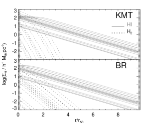
Figure 1: Surface density of HI and H₂ (solid and dashed lines, respectively) as a function of radius in units of the half-mass radius for randomly chosen galaxies in the Bow06 model, applying the KMT (top panel) and BR (bottom panel) SF laws.

In order to visualize the behaviour of the HI and H₂ components of the ISM of galaxies predicted in the models, we have taken the output of the original Bow06 model and postprocessed it to calculate the HI and H₂ surface density profiles based on the expressions above. Fig. 1 shows the surface density profiles of HI and H₂ for randomly chosen model spiral galaxies on applying the KMT (top panel) or the BR (bottom panel) laws. The HI extends to much larger radii than the H₂. This is a consequence of the total gas surface density dependence of the H${}_{2}/$HI ratio in both SF laws. Note that the KMT SF law gives a steeper decrease in the radial profile of H₂ compared to the BR SF law. The BR SF law depends on the surface density of gas and stars, through the disk pressure, while the KMT SF law depends on the surface density and metallicity of the gas.

We have compared our predictions for the size of the HI and H₂ disks with observations. The models predict a correlation between the HI isophotal radius, $l_{\rm HI}$, defined at a HI surface density of $1M_{\odot}\,\rm pc^{-2}$, and the enclosed HI mass, $M_{\rm HI}(l_{\rm HI})$, which is in very good agreement with observations, irrespective of the SF law applied. Both models predict $M_{\rm HI}(l_{\rm HI})/M_{\odot}\approx 2\times 10^{7}(l_{\rm HI}/\rm kpc)^{1.9}$, while the observed relation for Ursa Major is $M_{\rm HI}(l_{\rm HI})/M_{\odot}\approx 1.8\times 10^{7}(l_{\rm HI}/\rm kpc)^{1.86}$ (e.g. Verheijen & Sancisi 2001). On the other hand, the median of the relation between the exponential scale length of the H₂ and HI disks predicted by the model is $R_{\rm H_{2}}\approx 0.4\,R_{\rm HI}$, while the relation inferred by combining the observational results of Regan et al. (2001) and Verheijen & Sancisi (2001) is $R_{\rm H_{2}}=(0.44\pm 0.12)\,R_{\rm HI}$. The model agrees well with the observed relations indicating that, in general terms, the ISM of modelled galaxies looks realistic.

2.4 Consistent calculation or postprocessing?

Previous attempts to calculate the separate HI and H₂ contents of galaxies in a cosmological scenario have been made by postprocessing the output of existing semi-analytic models using specifically the BR SF prescription (e.g. Obreschkow et al. 2009a; Power et al. 2010). Here we show that a self-consistent calculation of the ISM of galaxies, in which the new SF laws are included in the model, is necessary throughout in order to explain the observed gas properties of galaxies. To do this we choose as an example the Bow06 model and the BR SF law.

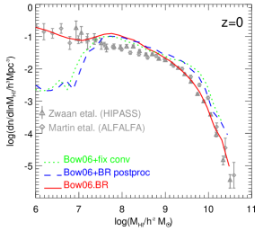
Figure 2: The HI mass function at $z=0$ for the original Bow06 model when a constant $M_{\rm mol}/M_{\rm cold}=0.27$ ratio is assumed (dotted line), when a variable conversion factor based on the BR pressure law is assumed (dotted line) and for the Bow06.BR model (solid line), where the BR SF law is consistently applied throughout the calculation. Symbols show observational results at $z=0$ from Zwaan et al. (2005) using HIPASS and Martin et al. (2010) using ALFALFA, as labelled.

Fig. 2 shows the HI MF in the original Bow06 model when a fixed conversion ratio of $M_{\rm mol}/M_{\rm cold}=0.27$ is assumed (dotted line; Baugh et al. 2004), when a variable conversion factor is calculated based on the BR pressure law (dashed line) and in the Bow06.BR model (solid line), where the BR SF law is applied consistently throughout the calculation. Symbols show a compilation of observational data. The original Bow06 model with a fixed H₂/HI conversion gives a poor match to the observed HI MF. Postprocessing the output of this model to implement a variable H₂/HI ratio gives a different prediction which still disagrees with the observations. If we consistently apply the BR SF law throughout the whole galaxy formation model, there is a substantial change in the model prediction which is also in much better agreement with the observations. These differences are mainly due to the fact that the SFR in the prescription of Bow06 scales linearly with the total cold gas mass (as in starbursts, see $\S 2.3$), while in the case of the BR SF law this dependence is non-linear. Note that a threshold in gas surface density below which galaxies are not allowed to form stars, as originally proposed by Kennicutt (1989) and as assumed in several other semi-analytic models (e.g. Croton et al. 2006; Tecce et al. 2010), produces a much less pronounced, but still present dip (see L11). Thus, the linearity of the SFR with cold gas mass is the main driver of the strong dip at low HI masses in the original model. Remarkably, our new modelling helps reproduce the observed number density even down to the current limits, $M_{\rm HI}\approx 10^{6}\,h^{-2}\,M_{\odot}$.

The new SF scheme to model the ISM of galaxies represents a step forward in understanding the gas content of galaxies. In the rest of the paper we make use of the models where the parameter-free SF laws are applied throughout the full calculation.

3 Scaling relations for the atomic and molecular contents of galaxies in the local universe

Here we present the model predictions for various scaling relations between H₂ and HI and other galaxy properties and compare with observations. In $\S 3.1$ we show how the H₂/HI ratio scales with stellar and cold gas mass. In $\S 3.2$ we present predictions for this ratio as a function of galaxy morphology, and in $\S 3.3$, we study dependence of the HI and H₂ masses on stellar mass.

3.1 The dependence of H₂/HI on galaxy mass

The prescriptions described in $\S 2$ that split the ISM into its atomic and molecular components enable the model to directly predict correlations between the H₂/HI ratio and galaxy properties. Fig. 3 shows the H₂/HI ratio as a function of stellar mass (top panels) and total cold gas mass (bottom panels) at $z=0$ for the Bow06 (solid lines) and the Bau05 (dashed lines) models using the BR and the KMT SF laws. The model predictions are compared to local observational estimates from Leroy et al. (2008). The errorbars on the model show the $10$ and $90$ percentiles of the model distribution in different mass bins. In the case of the observations, indicative errorbars on the H₂/HI estimate due to the uncertainty in the CO-H₂ conversion factor are shown at the top of the top-left panel (i.e. the difference in the value inferred for starbursts and the Milky-Way, $\approx 0.6$dex; see $\S 4.2$). Note that in this and subsequent figures where we compare with observations, we plot masses in units of $h^{-2}M_{\odot}$ to match observational units. For other plots we use the simulation units, $h^{-1}M_{\odot}$.

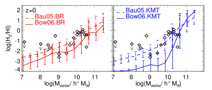
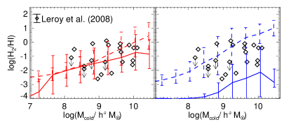
Figure 3: Molecular-to-atomic hydrogen ratio, H₂/HI, as a function of stellar mass (top panels) and total cold gas mass ($M_{\rm cold}=\rm He+HI+H_{2}$; bottom panels) for the two model variants, the Bow06 (solid lines) and Bau05 (dashed lines) models, when applying the BR (left panels) and the KMT (right panel) SF laws. Lines show the medians of the predicted distributions, while errorbars show the $10$% and $90$% percentiles. Grey symbols show observations of spiral and irregular galaxies from Leroy et al. (2008). Symbols with arrows represent upper limits in the observed sample. Indicative errorbars in the observational sample are shown in the bottom-left panel.

Leroy et al. estimated stellar masses from $3.6\mu$m luminosities, which were transformed into $K$-band luminosities using an empirical conversion. Stellar masses were then calculated from the relation of Bell et al. (2003) between the stellar mass-to-light ratio in the $K-$band and $B-V$ colour. Thus the error on the stellar mass might be as large as a factor of $1.5$ (considering the dispersion of $0.15$ dex in the $B-V$ vs. $K$-band relation).

The Bow06 model with the BR SF law predicts H₂/HI ratios which are in very good agreement with the observed ones. The Bow06.KMT model fails to match the observed H₂/HI ratios at all stellar and cold gas masses. This is due to the sharp decline of the radial profile of H₂ (see Fig. 1), which results in lower global H₂/HI ratios in disagreement with the observed ones. In the case of the Bow06.BR model, it might appear unsurprising that this model is in good agreement with the observed correlation given that it is based on the empirical correlation between H₂/HI and the hydrostatic pressure in the disk (see $\S 2$). However, it is only because we are able to reproduce other galaxy properties, such as stellar mass functions (see $\S 2$), gas fractions and, approximately galaxy sizes (L11), that we also predict the observed trend in the scaling relations shown in Fig. 3.

Both the Bau05.BR and Bau05.KMT models also give good agreement with the observed H₂/HI ratios. The success of the Bau05.KMT model, in contrast with the Bow06.KMT model, is mainly due to the higher gas masses and metallicites predicted in the former model. However, the Bau05.BR and Bau05.KMT models fail to reproduce the evolution of the $K$-band LF and the $z=0$ gas-to-luminosity ratios (see L11 for a complete discussion of the impact of each SF law on the two models).

3.2 The dependence of H₂/HI on galaxy morphology

It has been shown observationally that the ratio of H₂/HI masses correlates strongly with morphological type, with early-type galaxies characterised by higher H₂/HI ratios than late-type galaxies (e.g. Young & Knezek 1989; Bettoni et al. 2003; Lisenfeld et al. 2011). Fig. 4 shows the H₂/HI mass ratio as a function of the bulge-to-total luminosity ratio in the $B$-band, $B/T$, for different $B$-band absolute magnitude ranges for the Bow06.BR model. The right hand panel of Fig. 4, which shows the brightest galaxies, compares the model predictions with observations. All observational data have morphological types derived from a visual classification of the $B$-band images (de Vaucouleurs et al., 1991), and have also been selected in blue bands (e.g. Simien & de Vaucouleurs 1986; Weinzirl et al. 2009). The comparison with observational data is shown for galaxies in the model with $M_{B}-5\rm\,log($$h\rm)<-19$, which roughly corresponds to the selection criteria applied in the observational data. Note that we have plotted only galaxies in the model that have $M_{\rm HI}/M_{\star}\geq 10^{-3}$ and $M_{\rm H_{2}}/M_{\star}\geq 10^{-3}$, which correspond to the lowest HI and H₂ gas fractions detected in the observational data shown. The Bow06.BR model predicts a relation between the H₂/HI ratio and $B/T$ that is in good agreement with the observations. Note that, for the last bin, $B/T<0.2$, the model predicts slightly higher median H₂/HI ratios than the values inferred from observations. However, in all cases a constant CO$(1-0)$-H₂ conversion factor was assumed in the observational sample to infer the H₂ mass. This might not be a good approximation in the low-metallicity environments typical of irregular or late-type spirals, where the H₂ mass might be underestimated if a conversion factor typical of normal spiral galaxies is applied (e.g. Boselli et al. 2002; see $\S 4.2.1$ for a discussion).

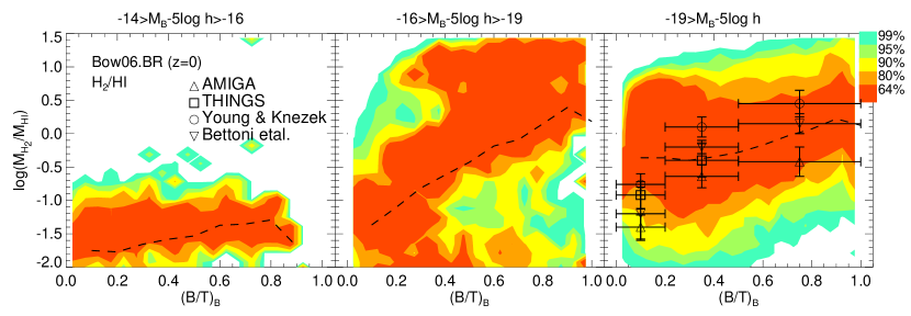
Figure 4: Molecular-to-atomic hydrogen mass ratio, $M_{\rm H_{2}}/M_{\rm HI}$, as a function of the bulge-to-total luminosity in the $B$-band, $(B/T)_{B}$, in the Bow06.BR model, for galaxies with absolute $B$-band magnitudes, $M_{B}-5\rm\,log(h)$, in the range indicated on top of each panel. Contours show the regions within which different volume-weighted percentages of the galaxies lie for a given $(B/T)_{B}$, with the scale shown by the key. For reference, the dashed line shows the median of the model distribution. Observational results from Young & Knezek (1989), Bettoni et al. (2003), Leroy et al. (2008) and Lisenfeld et al. (2011) are shown as symbols in the right-hand panel, and we combine them so that $B/T<0.2$ corresponds to Irr, Sm, Sd galaxies; $0.2<B/T<0.5$ corresponds to Sc, Sb, Sa galaxies; $B/T>0.5$ corresponds to E and S0 galaxies (see de Vaucouleurs et al. 1991 for a description of each morphological type).

The higher H₂/HI ratios in early-type galaxies can be understood in the context of the dependence of the H₂/HI ratio on gas pressure built into the BR SF law. Even though gas fractions in early-type galaxies are in general lower than in late-type galaxies, they are also systematically more compact than a late-type counterpart of the same mass (see Lagos et al. 2011), resulting in higher gas pressure, and consequently a higher H₂/HI ratio. Also note that there is a dependence on galaxy luminosity: faint galaxies typically have lower H₂/HI ratios than their bright counterparts. This is due to the contribution of the stellar surface density to the pressure, which increases in massive galaxies (see Eq 2).

3.3 The relation between HI, H₂ and stellar mass

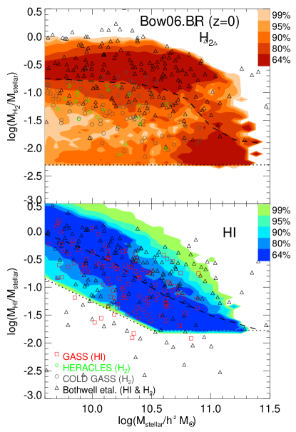
Figure 5: Top panel: Molecular hydrogen-to-stellar mass ratio as a function of stellar mass for the Bow06.BR model at $z=0$. The horizontal dotted line shows an approximate sensitivity limit below which CO(1-0) is not detected in the different molecular surveys. Contours show the regions within which different volume-weighted percentages of the galaxies lie for a given stellar mass and above the sensitivity limit, with the scale shown by the key. For reference, the dashed line shows the median of the model distributions. Observational data from the HERACLES survey (Leroy et al., 2009), the COLD GASS survey (Saintonge et al., 2011) and the literature compilation of Bothwell et al. (2009) are shown as symbols. Bottom panel: As in the top panel but for the atomic hydrogen-to-stellar mass ratio. Observational data from the GASS catalogue (Catinella et al., 2010) and the literature compilation of Bothwell et al. are shown as symbols. The dotted line shows the HI sensitivity limit of the GASS catalogue.

Another form of scaling relation often studied observationally is the atomic or molecular hydrogen-to-stellar mass ratio as a function of stellar mass. Recently, these relations have been reported for the atomic and molecular gas contents in a homogeneous sample of relatively massive galaxies by Catinella et al. (2010) and Saintonge et al. (2011), respectively, with the aim of establishing fundamental relations between the stellar content of galaxies and their cold gas mass. Fig. 5 shows these relations for the Bow06.BR model at $z=0$ compared to values reported for individual galaxies in these surveys with detected H₂ or HI, respectively. Also shown in the top panel are a data compilation from the literature presented in Bothwell et al. (2009) and individual galaxies from the HERA CO Line Extragalactic Survey (HERACLES; Leroy et al. 2009). Measurements of $M_{\rm H_{2}}/M_{\rm stellar}$ are subject to large errors (up to $0.25$ dex) given the uncertainty in the CO-H₂ conversion factor (see discussion in $\S 4.2.1$). Observed $M_{\rm HI}/M_{\rm stellar}$ ratios are more accurate given the direct detection of HI. Horizontal lines in Fig. 5 show representative observational sensitivity limits (which are not exactly the same in all samples). Contours show the regions where different fractions of galaxies in the model lie, normalized in bins of stellar mass. The contours are not very sensitive to the location of the sensitivity limits. The model predicts the right location and scatter of galaxies in these planes in contrast to previous models (see Saintonge et al. 2011 for a discussion). Note that the literature compilation of Bothwell et al. shows larger scatter than the HERACLES, GALEX Arecibo SDSS Survey (GASS) and CO Legacy Database for the GASS survey (COLD GASS). Saintonge et al. suggest that this is due to the inhomogeneity of the literature compilation.

The $M_{\rm H_{2}}/M_{\rm stellar}$ ratio in the model is only weakly correlated with stellar mass, in contrast to the $M_{\rm HI}/M_{\rm stellar}$ ratio which is strongly dependent on stellar mass, in agreement with the observations. The decrease in the $M_{\rm HI}/M_{\rm stellar}$ ratio with increasing stellar mass is the dominant factor in determining the positive relation between H₂/HI and stellar mass in Fig. 3 given the small variations of the $M_{\rm H_{2}}/M_{\rm stellar}$ ratio with stellar mass.

The predicted relation between $M_{\rm H_{2}}$ and $M_{\star}$ (top-panel of Fig. 5) is close to linear for galaxies with $M_{\rm H_{2}}/M_{\star}\gtrsim 0.05$. These galaxies lie on the active star-forming sequence in the $M_{\star}-\rm SFR$ plane (see L11), due to an approximately linear relation between $M_{\rm H_{2}}$ and SFR, although characterised by a large scatter (see $\S 4.2.3$). What drives the approximately constant $\rm SFR/$$M_{\star}$ and $M_{\rm H_{2}}/M_{\star}$ ratios for galaxies on the active star-forming sequence is the balance between accretion and outflows, mainly regulated by the timescale for gas to be reincorporated into the host halo after ejection by SNe (see L11 for details). In the case of HI, the model predicts that, for galaxies plotted in the bottom-panel of Fig. 5, the HI weakly correlates with stellar mass, $M_{\rm HI}\propto M^{0.15}_{\star}$, as a result of the feedback mechanisms included in the model.

4 Atomic and molecular hydrogen mass functions

The two-phase ISM scheme implemented in GALFORM (see $\S 2$) allows us to study the evolution of the HI and $\rm H_{2}$ in galaxies in terms of the MFs and their evolution. In the next two subsections we analyse the main mechanisms which shape the HI and $\rm H_{2}$ MFs and investigate how these interplay to determine the model predictions.

4.1 Atomic hydrogen mass function

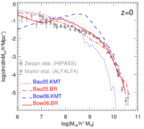
Figure 6: The HI mass function at $z=0$ for the Bau05.KMT (dotted line), Bau05.BR (dot-dashed line), Bow06.KMT (dashed line) and Bow06.BR (solid line) models. Symbols show the $z=0$ observational estimates from Zwaan et al. (2005) using HIPASS and from Martin et al. (2010) using ALFALFA, as labelled.

Fig. 6 shows the $z=0$ HI mass functions (HI MF) for the Bow06 and Bau05 models using the BR and the KMT SF laws, and observational results from Zwaan et al. (2005) and Martin et al. (2010).

With the BR SF law, both the Bow06 and Bau05 models give predictions which are in reasonable agreement with the observed HI MF. However, when applying the KMT SF law both models give a poor match to the observed HI MF, with the Bau05 model underpredicting the number density of massive HI galaxies, whilst the Bow06 model greatly overpredicts the abundance of galaxies around $M_{\rm HI}\sim 10^{9}h^{-2}\rm M_{\odot}$. The latter is expected from the poor agreement between the H₂/HI-stellar mass scaling relation predicted by Bow06.KMT and the observed one (Fig. 3). In the case of Bau05.KMT, the poor agreement is expected from the low gas-to-luminosity ratios reported by L11.

Cook et al. (2010) showed that, by including the BR SF law self-consistently in their semi-analytic model, the number density of low HI mass galaxies is substantially increased, in agreement with our results. However, in their model this effect is still not enough to bring the predictions into agreement with the observed HI MF. The overproduction of low mass galaxies is also seen in their predicted optical LFs, suggesting that the difference resides in the treatment of SN feedback and reionisation (see Bower et al. 2006; Benson & Bower 2010). In the case of the KMT SF law, there are no published results using the full SF law in semi-analytical models. Fu et al. (2010) implemented the H₂/HI metallicity- and gas surface density-dependence of the KMT SF law, but assumed a constant SF timescale for the molecular gas, instead of the original dependence on gas surface density (see Eq. 4). Furthermore, these authors compared their predictions to the observations of the HI MF only over the restricted range $10^{9}\lesssim M_{\rm HI}/h^{-2}M_{\odot}\lesssim 10^{10}$, one decade in mass compared to the five decades plotted in Fig. 6, so that it is hard to judge how well this KMT-like model really performs.

Given that neither of the models using the KMT SF law predict the right HI MF or H₂/HI scaling relations, and that the Bau05 model fails to predict the right $K$-band LF at $z>0.5$, we now focus on the Bow06.BR model when presenting the predictions for the gas contents of galaxies at low and high redshifts.

4.1.1 The composition of the HI mass function

The low mass end of the $z=0$ HI MF ($M_{\rm HI}\lesssim 10^{7}h^{-2}\rm M_{\odot}$), is dominated by satellite galaxies, as can be seen in the top panel of Fig. 7. Central galaxies contribute less to the number density in this mass range due to reionisation. Hot gas in halos with circular velocity $V_{\rm circ}<30\,\rm km\,s^{-1}$ is not allowed to cool at $z<10$, thereby suppressing the accretion of cold gas onto central galaxies hosted by these halos. These haloes have masses typically $M_{\rm halo}<10^{11}\,h^{-1}M_{\odot}$ (Benson, 2010). This suggests that the HI content of galaxies in isolation may lead to constraints on reionisation (Kim et al. in prep.). The HI MF of satellite galaxies does not show the dip at low HI masses observed in the HI MF of central galaxies because the satellites were mainly formed before reionisation. Galaxies of intermediate and high HI mass mainly correspond to central galaxies. The predominance in the HI MF of central and satellite galaxies in the high and low mass ends, respectively, is independent of the model adopted.

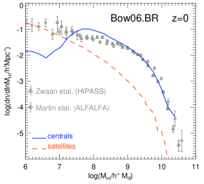
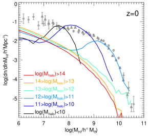
Figure 7: The HI mass function at $z=0$ in the Bow06.BR model, distinguishing between the contribution from central (solid line) and satellite (dashed line) galaxies in the top panel, and from galaxies hosted by DM halos of different masses, as labelled, in the bottom panel.

The Bow06.BR model slightly overpredicts the number density of galaxies in the mass range $3\times 10^{7}h^{-2}\rm M_{\odot}<M_{\rm HI}<3\times 10^{8}$$h^{-2}\rm M_{\odot}$. This is mainly due to the slightly larger radii of the model galaxies compared to observations (see L11), which leads to lower pressure within the galactic disk and therefore to a slight overestimate of the atomic hydrogen content.

The bottom panel of Fig. 7 shows the contribution to the HI MF from galaxies hosted by halos of different masses. The HI MF at intermediate and high HI masses, i.e. $M_{\rm HI}\gtrsim 5\times 10^{7}$$h^{-2}\rm M_{\odot}$, is dominated by galaxies hosted by low and intermediate mass DM halos, $M_{\rm halo}\lesssim 10^{12}h^{-1}\rm M_{\odot}$, while lower HI mass galaxies are primarily satellites in higher mass halos. This scale in the DM halo mass ($M_{\rm halo}\approx 10^{12}h^{-1}\rm M_{\odot}$) has been shown to be set by the efficient suppression of SF in higher mass DM haloes, mainly driven by AGN feedback which shuts down gas cooling (Kim et al., 2011). In lower mass halos, in which AGN feedback does not suppress gas cooling, the cold gas content scales with the stellar mass of the galaxy and with the mass of the host DM halo.

4.1.2 Evolution of the HI mass function

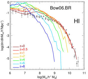
Figure 8: The HI mass functions for the Bow06.BR model at different redshifts, as labelled. For reference, we show the $z=0$ observational results from Zwaan et al. (2005) and Martin et al. (2010).

Fig. 8 shows the evolution of the HI MF from $z=8$ to $z=0$. There is a high abundance of low HI mass galaxies at high redshift. This reduces with declining redshift as gas is depleted mainly through quiescent SF and starbursts. The number density of galaxies with low HI masses, $M_{\rm HI}\lesssim 10^{7}h^{-2}\rm M_{\odot}$, increases with redshift, being a factor $4$ larger at $z=6$ than at $z=0$. The number density of HI galaxies with masses $10^{7}h^{-2}\rm M_{\odot}\lesssim M_{\rm HI}\lesssim 10^{8}{\it h}^{-2}\rm M_{\odot}$ increases by a factor of $2$ from $z=0$ to $z=1$, with little evolution to $z=4$. At $z>4$, the number density of galaxies in this mass range drops again. The high-mass end of the HI MF, $M_{\rm HI}\gtrsim 5\times 10^{8}h^{-2}\rm M_{\odot}$, grows hierarchically until $z\approx 1$, increasing in number density by more than two orders of magnitude. The evolution of the high-mass end tracks the formation of more massive haloes in which gas can cool, until AGN heating becomes important (at $z\approx 1$). At $z<1$ the high-mass end does not show appreciable evolution. The HI MF from the break upwards in mass is dominated by galaxies in intermediate mass halos. These are less affected by AGN feedback, driving the hierarchical growth in the number density in the high HI mass range. Higher mass halos, $M_{\rm halo}\gtrsim 10^{12}\,h^{-1}M_{\odot}$, are subject to AGN feedback, which suppresses the cooling flow and reduces the cold gas reservoir in the central galaxies of these haloes. Lower mass haloes, $M_{\rm halo}\lesssim 10^{11}\,h^{-1}M_{\odot}$, are susceptible to SNe feedback, which depletes the cold gas supply by heating the gas and returning it to the hot halo.

Note that our choice of parameters for reionisation affects mainly the low mass end of the MF at high redshifts. At $z=0$ the abundance of galaxies with $M_{\rm HI}\lesssim 10^{8}h^{-2}\rm M_{\odot}$ would be lower by a factor of $2$ if a lower photoionisation redshift cut of $z_{\rm reion}=6$ was assumed.

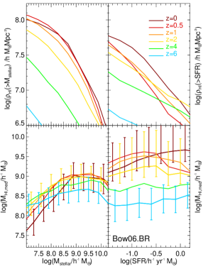
Figure 9: Top panels: cumulative HI mass density for galaxies in the Bow06.BR model with stellar masses (left panel) or SFRs (right panel) larger than a given value at different redshifts, as labelled. Bottom panels: median HI mass of galaxies as a function of stellar mass (left panel) and SFR (right panel). Errorbars correspond to the $10$ and $90$ percentiles of the distributions, and are shown for three different redshifts.

The characterisation of the HI MF at redshifts higher than $z\approx 0$ will be a difficult task in future observations. The first measurements will come from stacking of stellar mass- or SFR-selected galaxy samples, as has been done in the local Universe (e.g. Verheijen et al. 2007; Lah et al. 2007, 2009). Fig. 9 shows the cumulative HI mass per unit volume, $\rho_{\rm HI}$, at different redshifts for samples of galaxies in the Bow06.BR model that have stellar masses or SFRs larger than $M_{\rm stellar}$ or $\rm SFR$, respectively. The estimated $\rho_{\rm HI}$ from source stacking can be directly compared to our predictions for the same lower stellar mass or SFR limit. The median HI mass of galaxies as a function of stellar mass and SFR, is shown in the bottom-panels of Fig. 9. Errorbars represent the $10$ and $90$ percentiles of the distributions, and are shown for three different redshifts. The HI mass-stellar mass relation becomes shallower with increasing redshift, but the scatter around the median depends only weakly on redshift. The turnover of the median HI mass at $M_{\rm stellar}\gtrsim 10^{9}h^{-2}\,M_{\odot}$ is produced by AGN feedback that efficiently suppresses any further gas cooling onto massive galaxies and, consequently, their cold gas content is reduced. The HI mass is weakly correlated with SFR, particularly at high redshift. The median HI mass of galaxies spanning SFRs in the range plotted decreases with increasing redshift. This suggests that in order to detect low HI masses in observations at $z\approx 0.5-2$, stellar mass selected samples should be more effective than SFR selected samples. However, it would still be necessary to sample down to very low stellar masses ($M_{\rm stellar}>10^{8}\,h^{-1}\rm M_{\odot}$). Upcoming HI surveys using telescopes such as ASKAP and MeerKAT, will be able to probe down to these HI masses.

4.2 Molecular hydrogen mass function

The cold gas content is affected by SF, feedback processes, accretion of new cooled gas, but also by the evolution of galaxy sizes, given that our prescriptions to calculate the H₂ abundance depend explicitly on the gas density (see $\ 2.3$). Our aim is to disentangle which processes primarily determine the evolution of H₂ in galaxies.

4.2.1 The present-day $\rm CO(1-0)$ luminosity function

Observationally, the most commonly used tracer of the H₂ molecule is the CO molecule, and in particular, the $\rm CO(1-0)$ transition which is emitted in the densest, coldest regions of the ISM, where the H₂ is locked up. Given that in the model we estimate the H₂ content, we use a conversion factor to estimate the $\rm CO(1-0)$ emission for a given abundance of H₂,

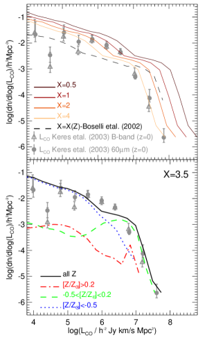
Figure 10: The $\rm CO(1-0)$ luminosity function at $z=0$ for the Bow06.BR model compared to the observational estimates of Keres et al. (2003) for $B$-band (triangles) and a $60\,\mu$m (filled circles) selected samples of galaxies. To calculate the $\rm CO(1-0)$ luminosities we assume a $\rm H_{2}$-to-CO conversion factor, $\rm X$, where $N_{\rm H_{2}}/\rm cm^{-2}=X\times 10^{-20}\,I_{\rm CO}/\rm K\,km\,s^{-1}$. In the top panel, solid lines show the model predictions using fixed values of X, as labelled, and the dashed line shows the LF using the metallicity-dependent conversion factor, $\rm X($$Z)$, of Boselli et al. (2002). In the bottom panel, the solid line shows the LF resulting from a conversion factor $X=3.5$ and the different lines show the contribution of galaxies in different metallicity ranges, as labelled, for this choice of X.

$$I_{\rm CO}/\rm K\,km\,s^{-1}=\frac{{\it N}_{\rm H_{2}}/\rm cm^{-2}}{\rm X\times 10^{-20}}.$$ (5)

Here $N_{\rm H_{2}}$ is the column density of H₂ and $I_{\rm CO}$ is the integrated CO$(1-0)$ line intensity per unit surface area. The value of $X$ has been inferred observationally in a few galaxies, mainly through virial estimations. Typical estimates for normal spiral galaxies range between $X\approx 2.0-3.5$ (e.g. Young & Scoville 1991; Boselli et al. 2002; Blitz et al. 2007). However, systematic variations in the value of $X$ are both, theoretically predicted and inferred observationally. For instance, theoretical calculations predict that low metallicities, characteristic of dwarf galaxies, or high densities and large optical depths of molecular clumps in starburst galaxies, should change X by a factor of up to $5-10$ in either direction (e.g. Bell et al. 2007; Meijerink et al. 2007; Bayet et al. 2009). Observations of dwarf galaxies favour larger conversion factors (e.g. $X\approx 7$; e.g. Boselli et al. 2002), while the opposite holds in starburst galaxies (e.g. $X\approx 0.5$; e.g. Meier & Turner 2004). This suggests a metallicity-dependent conversion factor X. However, estimates of the correlation between X and metallicity in nearby galaxies vary significantly, from finding no correlation, when virial equilibrium of giant molecular clouds (GMCs) is assumed (e.g. Young & Scoville 1991; Blitz et al. 2007), to correlations as strong as $X\propto(Z/Z_{\odot})^{-1}$, when the total gas content is inferred from the dust content on assuming metallicity dependent dust-to-gas ratios (e.g. Guelin et al. 1993; Boselli et al. 2002).

We estimate the $\rm CO(1-0)$ LF by using different conversion factors favoured by the observational estimates described above. The top panel of Fig. 10 shows the $\rm CO(1-0)$ LF at $z=0$ when different constant conversion factors are assumed (i.e. independent of galaxy properties; solid lines). Observational estimates of the $\rm CO(1-0)$ LF, made using a $B$-band and a $60\,\mu$m selected sample, are plotted using symbols (Keres et al., 2003). The model slightly underestimates the number density at $L^{\star}$ for $\rm X>1$, but gives good agreement at fainter and at brighter luminosities for sufficiently large values of X (such as the ones inferred in normal spiral galaxies). In the predicted $\rm CO(1-0)$ LF we include all galaxies with a $L_{\rm CO}>10^{3}\,\rm Jy\,km/s\,Mpc^{2}$, while the LFs from Keres et al. were inferred from samples of galaxies selected using $60\,\mu\rm m$ or $B$-band fluxes. These criteria might bias the LF towards galaxies with large amounts of dust or large recent SF. More data is needed from blind CO surveys in order to characterise the CO LF in non-biased samples of galaxies. This will be possible with new instruments such as the LMT.

In order to illustrate how much our predictions for the $\rm CO(1-0)$ LF at $z=0$ vary when adopting a metallicity-dependent conversion factor, $X(Z)$, inferred independently from observations, we also plot in the top panel of Fig. 10 the LF when the $X(Z)$ relation from Boselli et al. (2002) is adopted (dashed line), $\rm log({\it X})=0.5_{-0.2}^{+0.2}-1.02_{-0.05}^{+0.05}\rm log(\rm Z/Z_{\odot})$. Note that this correlation was determined using a sample of $12$ galaxies with $\rm CO(1-0)$ luminosities in quite a narrow range, $\rm L_{\rm CO}\approx 5\times 10^{5}-5\times 10^{6}$ $\rm Jy\,km/s\,Mpc^{2}$. On adopting this conversion factor, the model largely underestimates the break of the LF. This is due to the contribution of galaxies with different metallicities to the $\rm CO(1-0)$ LF, as shown in the bottom panel of Fig. 10. The faint-end is dominated by low-metallicity galaxies ($\rm Z<Z_{\odot}/3$), while high-metallicity galaxies ($\rm Z>Z_{\odot}/3$) dominate the bright-end. A smaller $X$ for low-metallicity galaxies combined with a larger $X$ for high-metallicity galaxies would give better agreement with the observed data. However, such a dependence of $X$ on metallicity is opposite to that inferred by Boselli et al.

By considering a dependence of $X$ on metallicity alone we are ignoring possible variations with other physical properties which could influence the state of GMCs, such as the interstellar far-UV radiation field and variations in the column density of gas (see for instance Pelupessy et al. 2006; Bayet et al. 2009; Pelupessy & Papadopoulos 2009; Papadopoulos 2010). Recently, Obreschkow et al. (2009b) showed that by using a simple phenomenological model to calculate the luminosity of different CO transitions, which includes information about the ISM of galaxies, the CO$(1-0)$ luminosity function of Fig. 10 can be reproduced. However, this modelling introduces several extra free parameters into the model which, in most cases, are not well constrained by observations. A more detailed calculation of the $\rm CO$ LF which takes into account the characteristics of the local ISM environment is beyond the scope of this paper and is addressed in a forthcoming paper (Lagos et al. 2011, in prep.).

For simplicity, in the next subsection we use a fixed $\rm CO(1-0)$-H₂ conversion factor of $X=3.5$ for galaxies undergoing quiescent SF and $X=0.5$ for those experiencing starbursts. In the case of galaxies undergoing both SF modes, we use $X=3.5$ and $X=0.5$ for the quiescent and the burst components, respectively, following the discussion above.

4.2.2 Evolution of the H₂ mass function

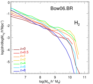
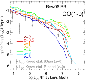
Figure 11: The H₂ MF (top panel) and the $\rm CO(1-0)$ LF (bottom panel) at different redshifts, as labelled, for the Bow06.BR model. Two fixed $\rm CO(1-0)$-H₂ conversion factors are assumed: $X=3.5$ for quiescent SF and $X=0.5$ for burst SF. For reference, we show the $\rm CO(1-0)$ LFs estimated at $z=0$ by Keres et al. (2003) from $B$-band and $60\,\mu$m-selected galaxy samples.

At high-redshift, measurements of the $\rm CO(J\rightarrow J-1)$ LF are not currently available. ALMA will, however, provide measurements of molecular emission lines in high redshift galaxies with high accuracy. We therefore present in Fig. 11 predictions for the H₂ MF and $\rm CO(1-0)$ LF up to $z=8$.

The high-mass end of the H₂ MF shows strong evolution from $z=8$ to $z=4$, with the number density of galaxies increasing by an order of magnitude. In contrast, the number density of low H₂ mass galaxies stays approximately constant over the same redshift range. From $z=4$ to $z=2$ the H₂ MF hardly evolves, with the number density of galaxies remaining the same over the whole mass range. From $z=2$ to $z=0$, the number density of massive galaxies decreases by an order of magnitude, while the low-mass end decreases only by a factor $\approx 3$. The peak in the number density of massive H₂ galaxies at $z=2-3$ coincides with the peak of the SF activity (see L11; Fanidakis et al. 2010), in which huge amounts of H₂ are consumed forming new stars. The following decrease in the number density at $z<2$ overlaps with strong galactic size evolution, where galaxies at lower redshift are systematically larger than their high redshift counterparts, reducing the gas surface density and therefore, the H₂ fraction. We return to this point in $\S$5. The peak in the number density of high H₂ mass galaxies at $z=2-3$ and the following decrease, contrasts with the monotonic increase in the number density of high HI mass galaxies with time, suggesting a strong evolution of the H₂/HI global ratio with redshift. We come back to this point in $\S 6$.

The evolution of the $\rm CO(1-0)$ LF with redshift is shown in the bottom panel of Fig. 11. Note that the $z=0$ LF is very similar to the one shown in the bottom panel of Fig. 10, in which we assume a fixed CO-H₂ conversion $X=3.5$ for all galaxies. This is due to the low number of starburst events at $z=0$. However, at higher redshifts, starbursts contribute more to the LF; the most luminous events at high redshift, in terms of CO luminosity, correspond to starbursts (see $\S 4.2.3$).

Recently Geach et al. (2011) compared the evolution of the observed molecular-to-(stellar plus molecular mass) ratio (which approximates to the gas-to-baryonic ratio if the HI fraction is small), $f_{\rm gas}=M_{\rm mol}/(M_{\rm stellar}+M_{\rm mol})$, with predictions for the Bow06.BR model at $z\leq 2$, and found that the model gives a good match to the observed $f_{\rm gas}$ evolution after applying the same observational selection cuts.

4.2.3 The IR-CO luminosity relation

One way to study the global relation between the SFR and the molecular gas mass in galaxies, and hence to constrain the SF law, is through the relation between the total IR luminosity, $L_{\rm IR}$, and the CO$(1-0)$ luminosity, $L_{\rm CO}$. We here define the total IR luminosity to be the integral over the rest-frame wavelength range $8-1000\mu$m, which approximates the total luminosity emitted by interstellar dust, free from contamination by starlight. In dusty star-forming galaxies, most of the UV radiation from young stars is absorbed by dust, and this dominates the heating of the dust, with only a small contribution to the heating from older stars. Under these conditions, and if there is no significant heating of the dust by an AGN, we expect that $L_{\rm IR}$ should be approximately proportional to the SFR, with a proportionality factor that depends mainly on the IMF. On the other hand, as already discussed, the CO$(1-0)$ luminosity has been found observationally to trace the molecular gas mass in local galaxies, albeit with a proportionality factor that is different in starbursts from quiescently star-forming galaxies. Observations suggest that sub-millimeter galaxies (SMGs) and QSOs at high redshift lie on a similar IR-CO luminosity relation to luminous IR galaxies (LIRGs) and ultra-luminous IR galaxies (ULIRGs) observed in the local Universe (see Solomon & Vanden Bout 2005 for a review). We investigate here whether our model predictions are consistent with these observational results.

We show in Fig. 12 the predicted IR-CO$(1-0)$ luminosity relation, $L_{\rm IR}-L^{\prime}_{\rm CO}$, for the Bow06.BR model at different redshifts, compared to observational data for different types of galaxies. The predicted CO$(1-0)$ luminosities for the model galaxies are calculated from their $H_{2}$ masses as in §4.2.1, using conversion factors $X=3.5$ for quiescent galaxies and $X=0.5$ for bursts. To facilitate the comparison with observations, we here express the CO luminosities $L^{\prime}_{\rm CO}$ in units of $\rm K\,km\,s^{-1}\,pc^{2}$, which corresponds to expressing the CO line intensity as a brightness temperature. We predict the IR luminosities of the model galaxies using the method described in Lacey et al. (2011b) and González et al. (2011) (see also Lacey et al. (2011a)), which uses a physical model for the dust extinction at each wavelength to calculate the total amount of stellar radiation absorbed by dust in each galaxy, which is then equal to its total IR luminosity. The dust model assumes a two-phase interstellar medium, with star-forming clouds embedded in a diffuse medium. The total mass of dust is predicted by GALFORM self-consistently from the cold gas mass and metallicity, assuming a dust-to-gas ratio which is proportional to the gas metallicity, while the radius of the diffuse dust component is assumed equal to that of the star-forming component, whether a quiescent disk or a burst, and is also predicted by GALFORM.

We show the model predictions in Fig. 12 separately for quiescent (left panel) and starburst galaxies (right panel), where quiescent galaxies are defined as those whose total SFR is dominated by SF taking place in the galactic disk (i.e. $\rm SFR_{\rm disk}>SFR_{\rm burst}$). Solid lines show the median of the predicted IR-CO relation at different redshifts, while errorbars represent the $10$ and $90$ percentiles of the distributions. To facilitate the comparison between quiescent and starburst galaxies, the typical IR luminosity at a CO luminosity of $10^{9}$ $h^{-2}\,\rm K\,km\,s^{-1}\,pc^{2}$ is shown as dotted lines in both panels. We see that the separate $L_{\rm IR}-L^{\prime}_{\rm CO}$ relations for quiescent and starburst galaxies depend only slightly on redshift, but that the relation for starbursts is offset to higher IR luminosities than for quiescent galaxies. There are two contributions to this offset in the model. The first is the different SF laws assumed in starbursts and in galaxy disks. By itself, this results in roughly 40 times larger IR luminosities at a given $H_{2}$ mass for starbursts. However, as already described, we also assume a CO-to-$H_{2}$ conversion factor $X$ which is 7 times smaller in starbursts, which causes an offset in the $L_{\rm IR}-L^{\prime}_{\rm CO}$ relation in the opposite sense. The combination of these two effects results in a net offset of roughly a factor of 6 in $L_{\rm IR}$ at a given $L^{\prime}_{\rm CO}$.

A similar bimodality in the IR-CO luminosity plane has also been inferred observationally by Genzel et al. (2010) and Combes et al. (2011). However, these results rely on inferring the CO(1-0) luminosities from higher CO transitions when the lowest transitions are not available, which could be significantly uncertain, as we discuss below (see also Ivison et al., 2011).

For comparison, we also plot in Fig. 12 a selection of observational data. We plot data for local LIRGs and for UV/optically-selected star-forming galaxies at $z\sim 1-2$ in the left panel, to compare with the model predictions for quiescent galaxies, and for local ULIRGs, SMGs at $z\sim 1-3$, and QSOs at $z\sim 0-6$ in the right panel, to compare with the model predictions for starbursts. We note that there are important uncertainties in the observational data plotted for high redshift ($z>1$) objects. For these, the IR luminosities are actually inferred from observations at a single wavelength ($24\mu$m or $850\mu$m), using an assumed shape for the SED of dust emission. (In addition, the Riechers (2011) data on $z>1$ QSOs are actually for FIR, i.e. $40-120\mu$m, luminosities, rather than total IR luminosities.) Furthermore, the CO$(1-0)$ luminosities for $z>1$ objects are in most cases also not direct measurements, but are instead inferred from measurements of higher CO transitions $J\rightarrow J-1$ (usually $4\rightarrow 3$ or $3\rightarrow 2$). The conversion from $L^{\prime}_{\rm CO}(J\rightarrow J-1)$ to $L^{\prime}_{\rm CO}(1-0)$ is usually done assuming that the brightness temperature of the CO line is independent of the transition $J\rightarrow J-1$, as would be the case if the CO lines are emitted from an optically thick medium in thermal equilibrium at a single temperature (as appears to be the case in local spiral galaxies). In this case, the luminosity $L^{\prime}_{\rm CO}$ is independent of the transition studied (Solomon & Vanden Bout, 2005). However, recent observations have shown different brightness temperatures for different CO transitions in some high-redshift galaxies (Danielson et al., 2010; Ivison et al., 2011). As a result, there could be large errors in the CO$(1-0)$ luminosities of high-redshift galaxies when they are inferred from higher transitions.

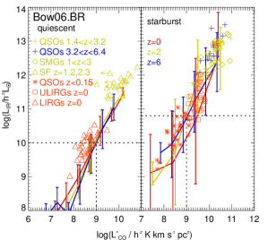
Figure 12: Infrared luminosity as a function of the CO($1-0$) luminosity for the Bow06.BR model at $z=0$ (red lines), $z=2$ (yellow lines) and $z=6$ (blue lines) for quiescent (left panel) and starburst galaxies (right panel). Solid lines show the median, while errorbars show the $10$ and $90$ percentiles of the distributions. To aid the comparison between the quiescent and starburst galaxies, dotted lines show the predicted median IR luminosity at $z=2$ for a CO luminosity of $10^{9}$ $h^{-2}\,\rm K\,km\,s^{-1}\,pc^{2}$. We also show the following observational data: local LIRGs from Gao & Solomon (2004) (triangles); local ULIRGs from Solomon et al. (1997) (squares); QSOs at $z\lesssim 0.15$ from Scoville et al. (2003), Evans et al. (2006) and Bertram et al. (2007) (asterisks); star-forming galaxies at $z\approx 1.2$ and $z\approx 2.3$ from Tacconi et al. (2010) and Genzel et al. (2010) (triangles); SMGs at $1\lesssim z\lesssim 3$ from Greve et al. (2005), Solomon & Vanden Bout (2005) and Tacconi et al. (2006) (diamonds); and QSOs at $1.4\lesssim z\lesssim 6.4$ from Riechers (2011) (crosses). Note that most of the observational data on the CO$(1-0)$ luminosity at high redshifts are inferred from the luminosities of higher CO transitions rather than being directly measured.

Comparing the model predictions for the IR-CO relation with the observational data, we see that the predictions for quiescent galaxies at $z=0$ are in broad agreement with the observations of nearby LIRGs, while at $z=2$ the model predicts partially the location of UV/optically-selected star-forming galaxies. In the case of starburst galaxies, the predicted relation agrees with the observations of low-redshift ULIRGs and high-redshift SMGs, and also with the observations of QSOs at both low and high redshift. The latter is consistent with the suggestion from observations that QSOs follow the same $L_{\rm IR}$-$L^{\prime}_{\rm CO}$ relation as starburst galaxies (e.g. Evans et al., 2006; Riechers, 2011). The model is thus able to explain the $L_{\rm IR}$-$L^{\prime}_{\rm CO}$ relation for all objects without needing to include any heating of dust by AGN. This also agrees with previous theoretical predictions which concluded that only higher CO transitions are affected by the presence of an AGN (e.g. Meijerink et al. 2007; Obreschkow et al. 2009b).

5 Evolution of scaling relations of the H₂ to $\rm HI$ ratio

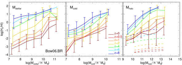
Figure 13: Molecular-to-atomic hydrogen ratio as a function of stellar mass (left panel), cold gas mass (middle panel) and DM halo mass (right panel) at different redshifts, as labelled, for the Bow06.BR model. Lines show the medians of the distributions, while errorbars show the $10$ to $90$ percentile ranges. For clarity, these errorbars are plotted only for three different redshifts. In the right panel, central and satellite galaxies are shown separately as solid and dashed lines, respectively. Errorbars are only shown for central galaxies in this panel.

Our model predicts that the HI and H₂ MFs are characterised by radically different evolution with redshift. This implies strong evolution of the H₂/HI ratio. In this section we analyse scaling relations of the H₂/HI ratio with galaxy properties and track the evolution of these relations towards high redshift with the aim of understanding what drives them.

Fig. 13 shows the median H₂$/$HI ratio as a function of stellar mass, cold gas mass and halo mass at different redshifts for the Bow06.BR model. Errorbars indicate the $10$ and $90$ percentiles of the model distribution in different mass bins. In the right panel, the predictions for satellite and central galaxies are shown separately as dashed and solid lines, respectively. For clarity, percentile ranges are only shown for central galaxies in this panel. In the case of satellites, the spread around the median is usually larger than it is for central galaxies.

Fig. 13 shows that the H₂/HI ratio correlates strongly with stellar and cold gas mass in an approximately power-law fashion. The normalisation of the correlation between H₂$/$HI and stellar mass (left panel of Fig. 13) evolves by two to three orders of magnitude from $z=8$ to $z=0$ towards smaller values. The evolution is milder (only $\approx 1.5$ dex) if one focuses instead on the correlation with cold gas mass. Interestingly, the slope of the correlation between the H₂$/$HI ratio and stellar or cold gas mass hardly evolves. The approximate scalings of the H₂/HI mass ratio against stellar and cold gas mass are:

$$\rm H_{2}/HI \approx 0.01\,\left(\frac{M_{\rm stellar}}{10^{10}{\it h}^{-1}\rm M_{\odot}}\right)^{0.8}\,(1+z)^{3.3},$$ (6)

$$\rm H_{2}/HI \approx 0.09\,\left(\frac{M_{\rm cold}}{10^{10}{\it h}^{-1}\rm M_{\odot}}\right)^{0.9}\,(1+z)^{2.4}.$$ (7)

Note that the relation with $M_{\rm stellar}$ is only valid up to $z=4$. At higher redshifts, the slope of the correlation becomes shallower. The relation with $M_{\rm cold}$, however, has the same slope up to $z=8$. The normalisation of the relation of H₂$/$HI with $M_{\rm stellar}$ has a stronger dependence on redshift compared to the relation with $M_{\rm cold}$. However, note that the distribution around the median is quite broad, as can be seen from the percentile range plotted in Fig. 13, so these expressions have be taken just as an illustration of the evolution of the model predictions.

The trend between the H₂$/$HI ratio of galaxies and host halo mass depends strongly on whether central or satellite galaxies are considered. In the case of central galaxies (solid lines in the right panel of Fig. 13), there is a correlation between the H₂$/$HI ratio and halo mass that becomes shallower with decreasing redshift in intermediate and high mass halos ($M_{\rm halo}>5\times 10^{11}h^{-1}\rm M_{\odot}$). This change in slope is mainly due to the fact that at lower redshift ($z\lesssim 1.5$), AGN feedback strongly suppresses SF in central galaxies hosted by halos in this mass range, so that the stellar mass-halo mass correlation also becomes shallower and with an increasing scatter. At high redshift, the stellar mass-halo mass correlation is tighter and steeper. In the case of satellite galaxies, the H₂$/$HI ratio does not vary with host halo mass, but exhibits a characteristic value that depends on redshift. The lower the redshift, the lower the characteristic H₂$/$HI ratio for satellites. Nonetheless, the spread around the median, in the case of satellite galaxies, is very large, i.e. of $1.5$ dex at $z=0$. The lack of correlation between the H₂$/$HI ratio and halo mass and the large scatter are due to the dependence of the H₂$/$HI ratio on galaxy properties (such as stellar and cold gas mass) rather than on the host halo mass.

In order to disentangle what causes the strong evolution of the H₂$/$HI ratio with redshift, we study the evolution of the galaxy properties that are directly involved in the calculation of the H₂$/$HI ratio. These are the disk size, cold gas mass and stellar mass, which together determine the hydrostatic pressure of the disk. Fig. 14 shows the H₂$/$HI ratio, the half-mass radius ($\rm r_{50}$), the cold gas mass, the stellar mass and the midplane hydrostatic pressure of the disk at $\rm r_{50}$, as functions of the cold baryonic mass of the galaxy, $M_{\rm bar}=M_{\rm stellar}+M_{\rm cold}$. These predictions are for the Bow06.BR model. Note that we only plot late-type galaxies (selected as those with a bulge-to-total stellar mass ratio $B/T<0.5$) as these dominate the cold gas density at any redshift.

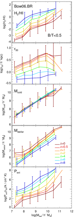
Figure 14: Molecular-to-atomic hydrogen ratio (top panel), half-mass radius, $\rm r_{50}$ (second panel), cold gas mass (third panel), stellar mass (fourth panel) and midplane hydrostatic pressure at $\rm r_{50}$ (bottom panel), as functions of the total cold baryonic mass in the galaxy (i.e. $M_{\rm bar}=M_{\rm stellar}+M_{\rm cold}$) at different redshifts (as labelled) for the Bow06.BR model. Solid lines show the medians of the distributions, while errorbars show the $10$ and $90$ percentiles, and for clarity are plotted only for three different redshifts.

In general, galaxies display strong evolution in size, moving towards larger radii at lower redshifts. However, this evolution takes place independently of galaxy morphology, implying that the galactic size evolution is caused by size evolution of the host DM halos (i.e. driven by mergers with other DM halos and accretion of dark matter onto halos). Note that the evolution in radius is about an order of magnitude from $z=6$ to $z=0$, which easily explains the evolution by two order of magnitudes in the H₂/HI ratio (which is $\propto P^{0.92}_{\rm ext}\propto\rm r^{-1.84}$). By increasing the disk size, the gas density and pressure decrease and therefore the molecular fraction decreases. The evolution in cold gas mass is mild enough so as not to significantly affect the H₂/HI ratio. Observationally, galaxies of the same rest-frame UV luminosity seem to be a factor $\approx 2-3$ smaller at $z\approx 6$ than at $z\approx 2$ (e.g. Bouwens et al. 2004; Oesch et al. 2010), in good agreement with the factor of $\approx 2-3$ evolution in size predicted by the Bow06.BR model (see Lacey et al. 2011b for a detailed comparison of sizes predicted by the model with the observed galaxy population).

Fig. 14 shows that the stellar mass of galaxies, at a given baryonic mass, increases with decreasing redshift and, therefore, the corresponding cold gas mass decreases. This drives the hydrostatic pressure to be reduced even further. The midplane hydrostatic pressure evaluated at $\rm r_{\rm 50}$, $P_{\rm ext}(\rm r_{\rm 50})/k_{\rm B}$ (bottom panel of Fig. 14), evolves by more than two orders of magnitude at a given $M_{\rm bar}$ over the redshift range plotted. Note that the typical values of $P_{\rm ext}(\rm r_{\rm 50})/k_{\rm B}$ predicted at $z=0$ are comparable to those reported in observations of nearby galaxies, $P_{\rm ext}/k_{\rm B}=10^{3}-10^{7}\,\rm cm^{-3}K$ (e.g. Blitz & Rosolowsky 2006; Leroy et al. 2008). At higher redshifts, the values of $P_{\rm ext}(\rm r_{\rm 50})$ also overlap with the range in which the $\Sigma_{\rm H_{2}}/\Sigma_{\rm HI}$-$P_{\rm ext}$ correlation has been constrained observationally at $z=0$.

The evolution in galactic size is therefore the main factor responsible for the predicted evolution in the H₂$/$HI ratio at fixed baryonic mass in the model, with a minor contribution from other properties which also contribute to determining this quantity (i.e. cold gas and stellar mass).

6 Cosmic evolution of the atomic and molecular gas densities

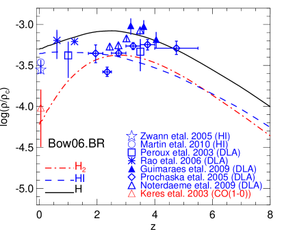
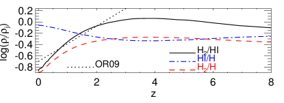
Figure 15: Top panel: Global density of all forms of neutral hydrogen gas (solid line), atomic hydrogen (dashed line) and molecular hydrogen (dotted-dashed line) in units of the critical density at $z=0$, as a function of redshift for the Bow06.BR model. Observational estimates of the HI mass density plotted are from Zwaan et al. (2005) and Martin et al. (2010) from the HI MF, and Péroux et al. (2003), Prochaska et al. (2005), Rao et al. (2006), Guimarães et al. (2009) and Noterdaeme et al. (2009) from DLAs. Also shown is the local Universe estimate of the H₂ mass density from Keres et al. (2003) using the $\rm CO(1-0)$ LF. Bottom panel: Global atomic-to-total neutral hydrogen (dot-dashed line), molecular-to-total neutral hydrogen (dashed line) and molecular-to-atomic hydrogen (solid line) mass ratios, as functions of redshift. For comparison, the evolution of the global molecular-to-atomic hydrogen ratio predicted by Obreschkow & Rawlings (2009) is shown as a dotted line.

The H₂/HI ratio depends strongly on galaxy properties and redshift. In this section we present predictions for the evolution of the global density of HI and H₂.

The top panel of Fig. 15 shows the evolution of the global comoving mean density of all forms of hydrogen (solid line), HI (dashed line) and H₂ (dot-dashed line), in units of the critical density at $z=0$, $\rho/\rho_{\rm c,z=0}$. Observational estimates of the HI and H₂ mass density at different redshifts and using different techniques are shown using symbols (see references in $\S 1$). If the reported values of $\rho_{\rm HI}$ and $\rho_{\rm H_{2}}$ include the contribution from helium, then we subtract this when plotting the data.

The model predicts local universe gas densities in good agreement with the observed ones, which is expected from the good agreement with the HI MF and $\rm CO(1-0)$ LF. At high redshift, the model predicts $\rho_{\rm HI}$ in good agreement with the observed density of HI inferred from damped-Ly$\alpha$ systems (DLAs). Note that in our model, by definition, the HI is attached to galaxies (see $\S 2$). However, recent simulations by Faucher-Giguère & Kereš (2011), Altay et al. (2010) and Fumagalli et al. (2011) suggest that DLAs might not correspond exclusively to HI gas attached to galaxies, but also to HI clumps formed during the rapid accretion of cold gas (e.g. Binney 1977; Haehnelt et al. 1998). Thus, the comparison between our predictions of $\rho_{\rm HI}$ and the values inferred from observations from DLAs has to be considered with caution in mind.

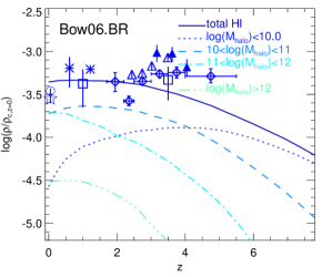
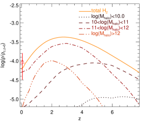
Figure 16: Global density of atomic hydrogen (top panel) and molecular hydrogen (bottom panel) in units of the critical density at $z=0$, as a function of redshift for the Bow06.BR model. The contributions from different DM halo mass ranges are shown by different lines as labelled. Observational estimates of the total HI and H₂ mass densities are also shown. Symbols correspond to different observations as labelled in Fig. 15.

At $z=0$ the HI mass density is much larger than that in H₂, due to the low molecular fractions in extended, low pressure galactic disks. At $z\approx 2$, where galactic disks are characterised by larger pressure and therefore, higher molecular fractions, the density of H₂ slightly exceeds that of HI. This H₂ domination extends up to $z\approx 5$, above which HI again becomes the principle form of neutral hydrogen. These transitions are clearly seen in the bottom panel of Fig. 15, where the evolution of the HI/H, H₂/H and H₂/HI global ratios are shown. Note that the peak of the H₂/HI global ratio is at $z\approx 3.5$. The predicted evolution of the H₂/HI global ratio differs greatly from the theoretical predictions reported previously by Obreschkow & Rawlings (2009, dotted line in the bottom panel of Fig. 15) and Power et al. (2010), which were obtained from postprocessed semi-analytic models (see $\S 2.4$). These authors reported a monotonic increase of the H₂/HI ratio with redshift, even up to global ratios of H₂/HI$\approx 10$. This difference with our results is due in part to resolution effects, since these papers used DM halos extracted from the Millennium simulation (see $\S 2.1$), and therefore only sample haloes with $M_{\rm halo}\geq 10^{10}\rm h^{-1}M_{\odot}$ at all redshifts. Consequently, these calculations were not able to resolve the galaxies that dominate the HI global density at high redshift, inferring an artificially high global H₂/HI ratio. We can confirm this assertion if we fix the halo mass resolution in the Bow06.BR model at $M_{\rm halo}=10^{10}\,h^{-1}M_{\odot}$, whereupon a global ratio of H₂/HI$\approx 7$ is attained at $z=8$. This is in better agreement with the value predicted by Obreschkow & Rawlings (2009), but is still $\sim 1.5$ times lower. We interpret this difference as being due to the postprocessing applied by Obreschkow et al. rather than the self-consistent calculation adopted here. We have already showed that postprocessing can lead to answers which differ substantially from the self consistent approach (see Fig 2). We can summarise the predicted evolution of the H₂/HI global ratio, $\rho_{\rm H_{2}}/\rho_{\rm HI}$, as being characterised by three stages,

$$\rm\rho_{\rm H_{2}}/\rho_{\rm HI} \approx 0.13\,(1+z)^{1.7}\quad{\rm for}\quad z\lesssim 2$$

$$\approx 0.45\,(1+z)^{0.6}\quad{\rm for}\quad 2\lesssim z\lesssim 4$$

$$\approx 3.7\,(1+z)^{-0.7}\quad{\rm for}\quad z\gtrsim 4.$$

Fig. 16 shows the contribution to $\rho_{\rm HI}$ (top panel) and $\rho_{\rm H_{2}}$ (bottom panel) from halos of different mass. The overall evolution of $\rho_{\rm HI}$ is always dominated by low and intermediate mass halos with $M_{\rm halo}<10^{12}\,h^{-1}\rm M_{\odot}$. At $z>1$, the contribution from halos with masses of $10^{11}\,h^{-1}\rm M_{\odot}<M_{\rm halo}<10^{12}\,h^{-1}\rm M_{\odot}$ quickly drops, and at $z>4$ the same happens with halos in the mass range $10^{10}\,h^{-1}\rm M_{\odot}<M_{\rm halo}<10^{11}\,h^{-1}\rm M_{\odot}$. At higher redshifts, low mass halos become the primary hosts of HI mass. In contrast, the evolution of $\rho_{\rm H_{2}}$ is always dominated by intermediate and high mass halos with $M_{\rm DM}>10^{11}\,h^{-1}\rm M_{\odot}$, supporting our interpretation of the evolution of the HI and H₂ MFs. This suggests that the weak clustering of HI galaxies reported by Meyer et al. (2007) and Basilakos et al. (2007) is mainly due to the fact that HI-selected galaxies are preferentially found in low mass halos, while in more massive halos the hydrogen content of galaxies has a larger contribution from H₂.

Note that the evolution of $\rho_{\rm HI}$ and $\rho_{\rm H_{2}}$ with redshift is weaker than the evolution of the SFR density, $\rho_{\rm SFR}$. As L11 reported, $\rho_{\rm SFR}$ increases by a factor of $\approx 15$ from $z=0$ to $z=3$ (the predicted peak of the SF activity). On the other hand, $\rho_{\rm H_{2}}$ evolves by a factor of $\approx 7$ from $z=0$ to $z=3$ (where the H₂ density peaks), while $\rho_{\rm HI}$ evolves weakly, decreasing by a factor only of $1.5$ from $z=0$ to $z=5$. The difference in the redshift evolution between $\rho_{\rm H_{2}}$ and $\rho_{\rm SFR}$ is due to the contribution from starbursts to the latter at $z>2$, that drops quickly at lower redshifts. This leads to a larger decrease in the global $\rho_{\rm SFR}$ compared to $\rho_{\rm H_{2}}$. We remind the reader that we assume different SF laws for starbursts and quiescent SF, and therefore, by construction, different gas depletion timescales (see §2.3).

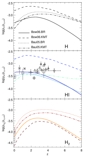
Figure 17: Global density of all forms of neutral H (top panel), HI (middle panel) and H₂ (bottom panel) in units of the critical density at $z=0$, as a function of redshift for the Bow06.BR, Bow06.KMT, Bau05.BR and Bau05.KMT models, as labelled in the top panel. Symbols show observational estimates, as labelled in Fig. 15.

In order to gain an impression of how much the predicted global density evolution can change with the modelling of SF, Fig. 17 shows the global density evolution of the neutral H, HI and H₂ for the Bau05.BR, Bau05.KMT, Bow06.BR and Bow06.KMT models. The former three models predict very similar global density evolution of HI at $z<4$, while at higher redshifts the Bau05.KMT model predicts larger global densities mainly due to the metallicity dependence of the H₂/HI ratio in the KMT SF law (see Eq. 4) and the typically lower gas metallicities in high redshift galaxies. However, the Bow06.KMT model predicts a global density of HI offset by a factor of $4$ with respect to the observational estimates and the other models over the whole redshift range. This is caused by the large overprediction of the number density of intermediate HI mass galaxies by this model (Fig. 6). In the case of the global density of H₂, all the models predict a similar redshift peak at $z\approx 3-4$, but with an offset in the maximum density attained.

7 Summary and conclusions

We have presented predictions for the HI and H₂ content of galaxies and their evolution with redshift in the context of galaxy formation in the $\Lambda$CDM framework. We use the extension of the GALFORM semi-analytic model implemented by Lagos et al. (2010, L11), in which the neutral hydrogen in the ISM of galaxies is split into its atomic and molecular components. To do that we have used either the empirical correlation of Blitz & Roslowsky (2006, BR), between the H₂/HI ratio and the hydrostatic pressure of the disk or the formalism of Krumholz et al. (2009, KMT) of molecule formation on dust grains balanced by UV dissociation. We assume that the SFR depends directly on the H₂ content of galaxies, as suggested by observational results for nearby galaxies (e.g. Wong & Blitz 2002; Solomon & Vanden Bout 2005; Bigiel et al. 2008; Schruba et al. 2010). We do not change any other model parameter, so as to isolate the consequences of changing the SF law on the model predictions.

We study the evolution of HI and H₂ predicted by two models, those of Baugh et al. (2005, Bau05) and Bower et al. (2006, Bow06), after applying the BR or the KMT SF law prescriptions. When applying the BR SF law, we find that the Bau05 and the Bow06 models predict a present-day HI MF in broad agreement with observations by Zwaan et al. (2005) and Martin et al. (2010), and a relation between the H₂/HI ratio and stellar and cold gas mass in broad agreement with Leroy et al. (2008). When applying the KMT SF law, the two models fail to predict the observed HI MF at $z=0$. Moreover, L11 find that the Bau05 model fails to predict the observed $K$-band LF at $z>0.5$, regardless of the SF law assumed. Hence, we select as our best model that of Bow06 with the BR SF law applied (Bow06.BR). This model predicts local Universe estimates of the HI and H₂ MFs, scaling relations of the H₂/HI, $M_{\rm H_{2}}/M_{\rm stellar}$ and $M_{\rm HI}/M_{\rm stellar}$ ratios with galaxy properties, and also the IR-CO luminosity relation in reasonable agreement with observations, but also gives good agreement with stellar masses, optical LFs, gas-to-luminosity ratios, among others (see L11 for a full description of the predictions of the GALFORM model when changing the SF law and Fanidakis et al. 2010 for predictions of this model for the AGN population). We show that the new SF law applied is a key model component to reproduce the local HI MF at intermediate and low HI masses given that it reduces SF and, therefore, SNe feedback, allowing the survival of larger gas reservoirs.

Using the Bow06.BR model, we can predict the evolution of the HI and H₂ MFs. We find that the evolution of HI is characterised by a monotonic increase in the number density of massive galaxies with decreasing redshift. For H₂, the number density of massive galaxies increases from $z=8$ to $z=4$, followed by very mild evolution down to $z=2$. At $z<2$, the number density in this range drops quickly. These radical differences in the HI and H₂ MF evolution are due to the strong evolution in the H₂/HI ratio with redshift, due to the dependence on galaxy properties. We also present predictions for the HI mass-stellar mass and HI mass-SFR relations, and for the cumulative HI mass density of stacked samples of galaxies selected by stellar mass or SFR at different redshifts, which is relevant to the first observations of HI expected at high redshift.

At a given redshift, the H₂/HI ratio strongly depends on the stellar and cold gas masses. The normalisation of the correlation evolves strongly with redshift, increasing by two orders of magnitude from $z=0$ up to $z=8$, in contrast with the very mild evolution in the slope of the correlations. We also find that the H₂/HI ratio correlates with halo mass only for central galaxies, where the slope and normalization of the correlation depends on redshift. For satellite galaxies, no correlation with the host halo mass is found, which is a result of the weak correlation between satellite galaxy properties and their host halo mass. We find that the main mechanism driving the evolution of the amplitude of the correlation between the H₂/HI ratio and stellar and cold gas mass, and with halo mass in the case of central galaxies, is the size evolution of galactic disks. Lower-redshift galaxies are roughly an order of magnitude larger than $z=8$ galaxies with the same baryonic mass (cold gas and stellar mass).

Finally, we studied the cosmic density evolution of HI and H₂, and find that the former is characterised by very mild evolution with redshift, in agreement with observations of DLAs (e.g. Péroux et al. 2003; Noterdaeme et al. 2009), while the density of H₂ increases by a factor of $7$ from $z\approx 0$ to $z\approx 3$. We also predict that H₂ slightly dominates over the HI content of the universe between $z\approx 2-4$ (with a peak of $\rho_{\rm H_{2}}/\rho_{\rm HI}\approx 1.2$ at $z\approx 3.5$), and that it is preferentially found in intermediate mass DM halos. On the other hand, we find that the HI is mainly contained in low mass halos. The global H₂/HI density ratio evolution with redshift is characterised by a rapid increase from $z=0$ to $z=2$ as $\rho_{\rm H_{2}}/\rho_{\rm HI}\propto\rm(1+z)^{1.7}$, followed by a slow increase at $2<z<4$ as $\rho_{\rm H_{2}}/\rho_{\rm HI}\propto\rm(1+z)^{0.6}$, to finally decrease slowly with increasing redshift at $z>4$ as $\rho_{\rm H_{2}}/\rho_{\rm HI}\propto\rm(1+z)^{-0.7}$. We conclude that previous studies (Obreschkow & Rawlings 2009; Power et al. 2010) overestimated this evolution due in part to halo mass resolution effects, as the galaxies which dominate the HI density at $z\gtrsim 2$ were not resolved in these calculations.

The results of this paper suggest radically different evolution of the cosmic densities of HI and H₂, as well as a strong evolution in the H₂/HI ratio in galaxies. The next generation of radio and submm telescopes (such as ASKAP, MeerKAT, SKA, LMT and ALMA) will reveal the neutral gas content of the Universe and galaxies up to very high-redshifts, and will be able to test the predictions made here.

References

- Almeida et al. (2007) Almeida C., Baugh C. M., Lacey C. G., 2007, MNRAS, 376, 1711
- Altay et al. (2010) Altay G., Theuns T., Schaye J., Crighton N. H. M., Dalla Vecchia C., 2010, ApJL accepted, ArXiv:1012.4014
- Basilakos et al. (2007) Basilakos S., Plionis M., Kovač K., Voglis N., 2007, MNRAS, 378, 301
- Baugh (2006) Baugh C. M., 2006, Reports on Progress in Physics, 69, 3101
- Baugh et al. (2004) Baugh C. M., Lacey C. G., Frenk C. S., Benson A. J., Cole S., Granato G. L., Silva L., Bressan A., 2004, New Astron. Rev., 48, 1239
- Baugh et al. (2005) Baugh C. M., Lacey C. G., Frenk C. S., Granato G. L., Silva L., Bressan A., Benson A. J., Cole S., 2005, MNRAS, 356, 1191
- Bayet et al. (2009) Bayet E., Viti S., Williams D. A., Rawlings J. M. C., Bell T., 2009, ApJ, 696, 1466
- Bell et al. (2003) Bell E. F., McIntosh D. H., Katz N., Weinberg M. D., 2003, ApJS, 149, 289
- Bell et al. (2007) Bell T. A., Viti S., Williams D. A., 2007, MNRAS, 378, 983
- Benson (2010) Benson A. J., 2010, Phys. Rep., 495, 33
- Benson & Bower (2010) Benson A. J., Bower R., 2010, MNRAS, 405, 1573
- Benson et al. (2003) Benson A. J., Bower R. G., Frenk C. S., Lacey C. G., Baugh C. M., Cole S., 2003, ApJ, 599, 38
- Bertram et al. (2007) Bertram T., Eckart A., Fischer S., Zuther J., Straubmeier C., Wisotzki L., Krips M., 2007, A&A, 470, 571
- Bettoni et al. (2003) Bettoni D., Galletta G., García-Burillo S., 2003, A&A, 405, 5
- Bigiel et al. (2008) Bigiel F., Leroy A., Walter F., Brinks E., de Blok W. J. G., Madore B., Thornley M. D., 2008, AJ, 136, 2846
- Bigiel et al. (2011) Bigiel F., Leroy A. K., Walter F., Brinks E., de Blok W. J. G., Kramer C., Rix H. W., Schruba A. et al, 2011, ApJ, 730, L13+
- Binney (1977) Binney J., 1977, ApJ, 215, 483
- Blitz et al. (2007) Blitz L., Fukui Y., Kawamura A., Leroy A., Mizuno N., Rosolowsky E., 2007, Protostars and Planets V, 81
- Blitz & Rosolowsky (2006) Blitz L., Rosolowsky E., 2006, ApJ, 650, 933
- Booth et al. (2009) Booth R. S., de Blok W. J. G., Jonas J. L., Fanaroff B., 2009, ArXiv:0910.2935
- Boselli et al. (2002) Boselli A., Lequeux J., Gavazzi G., 2002, A&A, 384, 33
- Bothwell et al. (2009) Bothwell M. S., Kennicutt R. C., Lee J. C., 2009, MNRAS, 400, 154
- Bouwens et al. (2004) Bouwens R. J., Illingworth G. D., Blakeslee J. P., Broadhurst T. J., Franx M., 2004, ApJ, 611, L1
- Bower et al. (2006) Bower R. G., Benson A. J., Malbon R., Helly J. C., Frenk C. S., Baugh C. M., Cole S., Lacey C. G., 2006, MNRAS, 370, 645
- Catinella et al. (2010) Catinella B., Schiminovich D., Kauffmann G., Fabello S., Wang J., Hummels C., Lemonias J., Moran S. M. et al, 2010, MNRAS, 403, 683
- Cattaneo et al. (2008) Cattaneo A., Dekel A., Faber S. M., Guiderdoni B., 2008, MNRAS, 389, 567
- Chang et al. (2010) Chang T., Pen U., Bandura K., Peterson J. B., 2010, Nature, 466, 463
- Cole et al. (2000) Cole S., Lacey C. G., Baugh C. M., Frenk C. S., 2000, MNRAS, 319, 168
- Combes et al. (2011) Combes F., García-Burillo S., Braine J., Schinnerer E., Walter F., Colina L., 2011, A&A, 528, 124
- Cook et al. (2010) Cook M., Evoli C., Barausse E., Granato G. L., Lapi A., 2010, MNRAS, 402, 941
- Croton et al. (2006) Croton D. J., Springel V., White S. D. M., De Lucia G., Frenk C. S., Gao L., Jenkins A., Kauffmann G. et al, 2006, MNRAS, 365, 11
- Daddi et al. (2010) Daddi E., Bournaud F., Walter F., Dannerbauer H., Carilli C. L., Dickinson M., Elbaz D., Morrison G. E. et al, 2010, ApJ, 713, 686
- Danielson et al. (2010) Danielson A. L. R., Swinbank A. M., Smail I., Cox P., Edge A. C., Weiss A., Harris A. I., Baker A. J. et al, 2010, MNRAS, 1565
- de Vaucouleurs et al. (1991) de Vaucouleurs G., de Vaucouleurs A., Corwin Jr. H. G., Buta R. J., Paturel G., Fouque P., 1991, S&T, 82, 621
- Dutton et al. (2010) Dutton A. A., van den Bosch F. C., Dekel A., 2010, MNRAS, 405, 1690
- Elmegreen (1993) Elmegreen B. G., 1993, ApJ, 411, 170
- Evans et al. (2006) Evans A. S., Solomon P. M., Tacconi L. J., Vavilkin T., Downes D., 2006, AJ, 132, 2398
- Fanidakis et al. (2010) Fanidakis N., Baugh C. M., Benson A. J., Bower R. G., Cole S., Done C., Frenk C. S., Hickox R. C. et al, 2010, MNRAS submitted, ArXiv:1011.5222
- Faucher-Giguère & Kereš (2011) Faucher-Giguère C., Kereš D., 2011, MNRAS, 412, L118
- Fu et al. (2010) Fu J., Guo Q., Kauffmann G., Krumholz M. R., 2010, MNRAS, 409, 515
- Fumagalli et al. (2011) Fumagalli M., Prochaska J. X., Kasen D., Dekel A., Ceverino D., Primack J. R., 2011, MNRAS submitted, ArXiv:1103.2130
- Gao & Solomon (2004) Gao Y., Solomon P. M., 2004, ApJ, 606, 271
- Geach et al. (2009) Geach J. E., Smail I., Coppin K., Moran S. M., Edge A. C., Ellis R. S., 2009, MNRAS, 395, L62
- Geach et al. (2011) Geach J. E., Smail I., Moran S. M., MacArthur L. A., Lagos C. d. P., Edge A. C., 2011, ApJ, 730, L19+
- Genzel et al. (2010) Genzel R., Tacconi L. J., Gracia-Carpio J., Sternberg A., Cooper M. C., Shapiro K., Bolatto A., Bouché N. et al, 2010, MNRAS, 407, 2091
- Giovanelli et al. (2005) Giovanelli R., Haynes M. P., Kent B. R., Perillat P., Saintonge A., Brosch N., Catinella B., Hoffman G. L. et al, 2005, AJ, 130, 2598
- González et al. (2011) González J. E., Lacey C. G., Baugh C. M., Frenk C. S., 2011, MNRAS, 413, 749
- González et al. (2009) González J. E., Lacey C. G., Baugh C. M., Frenk C. S., Benson A. J., 2009, MNRAS, 397, 1254
- Granato et al. (2000) Granato G. L., Lacey C. G., Silva L., Bressan A., Baugh C. M., Cole S., Frenk C. S., 2000, ApJ, 542, 710
- Greve et al. (2005) Greve T. R., Bertoldi F., Smail I., Neri R., Chapman S. C., Blain A. W., Ivison R. J., Genzel R. et al, 2005, MNRAS, 359, 1165
- Guelin et al. (1993) Guelin M., Zylka R., Mezger P. G., Haslam C. G. T., Kreysa E., Lemke R., Sievers A. W., 1993, A&A, 279, L37
- Guimarães et al. (2009) Guimarães R., Petitjean P., de Carvalho R. R., Djorgovski S. G., Noterdaeme P., Castro S., Poppe P. C. D. R., Aghaee A., 2009, A&A, 508, 133
- Haehnelt et al. (1998) Haehnelt M. G., Steinmetz M., Rauch M., 1998, ApJ, 495, 647
- Hughes et al. (2010) Hughes D. H., Jáuregui Correa J., Schloerb F. P., Erickson N., Romero J. G., Heyer M., Reynoso D. H., Narayanan G., Perez-Grovas A. S., Souccar K., Wilson G., Yun M., 2010, in Society of Photo-Optical Instrumentation Engineers (SPIE) Conference Series, Vol. 7733, Society of Photo-Optical Instrumentation Engineers (SPIE) Conference Series
- Ivison et al. (2011) Ivison R. J., Papadopoulos P. P., Smail I., Greve T. R., Thomson A. P., Xilouris E. M., Chapman S. C., 2011, MNRAS, 46
- Johnston et al. (2008) Johnston S., Taylor R., Bailes M., Bartel N., Baugh C., Bietenholz M., Blake C., Braun R. et al, 2008, Experimental Astronomy, 22, 151
- Kennicutt (1983) Kennicutt Jr. R. C., 1983, ApJ, 272, 54
- Kennicutt (1989) —, 1989, ApJ, 344, 685
- Kennicutt (1998) —, 1998, ApJ, 498, 541
- Keres et al. (2003) Keres D., Yun M. S., Young J. S., 2003, ApJ, 582, 659
- Kim et al. (2011) Kim H.-S., Baugh C. M., Benson A. J., Cole S., Frenk C. S., Lacey C. G., Power C., Schneider M., 2011, MNRAS, 414, 2367
- Kregel et al. (2002) Kregel M., van der Kruit P. C., de Grijs R., 2002, MNRAS, 334, 646
- Kroupa (2001) Kroupa P., 2001, MNRAS, 322, 231
- Krumholz et al. (2009) Krumholz M. R., McKee C. F., Tumlinson J., 2009, ApJ, 699, 850
- Lacey et al. (2011a) Lacey C. G., Baugh C. M., Frenk C. S., 2011a. In preparation
- Lacey et al. (2011b) Lacey C. G., Baugh C. M., Frenk C. S., Benson A. J., 2011b, MNRAS, 45
- Lacey et al. (2008) Lacey C. G., Baugh C. M., Frenk C. S., Silva L., Granato G. L., Bressan A., 2008, MNRAS, 385, 1155
- Lagos et al. (2008) Lagos C. D. P., Cora S. A., Padilla N. D., 2008, MNRAS, 388, 587
- Lagos et al. (2011) Lagos C. D. P., Lacey C. G., Baugh C. M., Bower R. G., Benson A. J., 2011, MNRAS, 1148
- Lah et al. (2007) Lah P., Chengalur J. N., Briggs F. H., Colless M., de Propris R., Pracy M. B., de Blok W. J. G., Fujita S. S. et al, 2007, MNRAS, 376, 1357
- Lah et al. (2009) Lah P., Pracy M. B., Chengalur J. N., Briggs F. H., Colless M., de Propris R., Ferris S., Schmidt B. P. et al, 2009, MNRAS, 399, 1447
- Leroy et al. (2009) Leroy A. K., Walter F., Bigiel F., Usero A., Weiss A., Brinks E., de Blok W. J. G., Kennicutt R. C. et al, 2009, AJ, 137, 4670
- Leroy et al. (2008) Leroy A. K., Walter F., Brinks E., Bigiel F., de Blok W. J. G., Madore B., Thornley M. D., 2008, AJ, 136, 2782
- Lisenfeld et al. (2011) Lisenfeld U., Espada D., Verdes-Montenegro L., Kuno N., Leon S., Sabater J., Sato N., Sulentic S. et al, 2011, Submitted to A&A
- Mac Low & Klessen (2004) Mac Low M., Klessen R. S., 2004, Reviews of Modern Physics, 76, 125
- Martin et al. (2010) Martin A. M., Papastergis E., Giovanelli R., Haynes M. P., Springob C. M., Stierwalt S., 2010, ApJ, 723, 1359
- McKee & Ostriker (2007) McKee C. F., Ostriker E. C., 2007, ARA&A, 45, 565
- Meier & Turner (2004) Meier D. S., Turner J. L., 2004, AJ, 127, 2069
- Meijerink et al. (2007) Meijerink R., Spaans M., Israel F. P., 2007, A&A, 461, 793
- Meyer et al. (2007) Meyer M. J., Zwaan M. A., Webster R. L., Brown M. J. I., Staveley-Smith L., 2007, ApJ, 654, 702
- Meyer et al. (2004) Meyer M. J., Zwaan M. A., Webster R. L., Staveley-Smith L., Ryan-Weber E., Drinkwater M. J., Barnes D. G., Howlett M. et al, 2004, MNRAS, 350, 1195
- Narayanan et al. (2009) Narayanan D., Cox T. J., Hayward C. C., Younger J. D., Hernquist L., 2009, MNRAS, 400, 1919
- Norberg et al. (2001) Norberg P., Baugh C. M., Hawkins E., Maddox S., Peacock J. A., Cole S., Frenk C. S., Bland-Hawthorn J. et al, 2001, MNRAS, 328, 64
- Noterdaeme et al. (2008) Noterdaeme P., Ledoux C., Petitjean P., Srianand R., 2008, A&A, 481, 327
- Noterdaeme et al. (2009) Noterdaeme P., Petitjean P., Ledoux C., Srianand R., 2009, A&A, 505, 1087
- Obreschkow et al. (2009a) Obreschkow D., Croton D., De Lucia G., Khochfar S., Rawlings S., 2009a, ApJ, 698, 1467
- Obreschkow et al. (2009b) Obreschkow D., Heywood I., Klöckner H.-R., Rawlings S., 2009b, ApJ, 702, 1321
- Obreschkow & Rawlings (2009) Obreschkow D., Rawlings S., 2009, ApJ, 696, L129
- Oesch et al. (2010) Oesch P. A., Bouwens R. J., Carollo C. M., Illingworth G. D., Trenti M., Stiavelli M., Magee D., Labbé I. et al, 2010, ApJ, 709, L21
- Okamoto et al. (2008) Okamoto T., Gao L., Theuns T., 2008, MNRAS, 390, 920
- Papadopoulos (2010) Papadopoulos P. P., 2010, ApJ, 720, 226
- Parkinson et al. (2008) Parkinson H., Cole S., Helly J., 2008, MNRAS, 383, 557
- Pelupessy & Papadopoulos (2009) Pelupessy F. I., Papadopoulos P. P., 2009, ApJ, 707, 954
- Pelupessy et al. (2006) Pelupessy F. I., Papadopoulos P. P., van der Werf P., 2006, ApJ, 645, 1024
- Péroux et al. (2003) Péroux C., McMahon R. G., Storrie-Lombardi L. J., Irwin M. J., 2003, MNRAS, 346, 1103
- Power et al. (2010) Power C., Baugh C. M., Lacey C. G., 2010, MNRAS, 406, 43
- Prochaska et al. (2005) Prochaska J. X., Herbert-Fort S., Wolfe A. M., 2005, ApJ, 635, 123
- Rao et al. (2006) Rao S. M., Turnshek D. A., Nestor D. B., 2006, ApJ, 636, 610
- Rauch (1998) Rauch M., 1998, ARA&A, 36, 267
- Regan et al. (2001) Regan M. W., Thornley M. D., Helfer T. T., Sheth K., Wong T., Vogel S. N., Blitz L., Bock D. C.-J., 2001, ApJ, 561, 218
- Riechers (2011) Riechers D. A., 2011, ApJ, 730, 108
- Roychowdhury et al. (2009) Roychowdhury S., Chengalur J. N., Begum A., Karachentsev I. D., 2009, MNRAS, 397, 1435
- Saintonge et al. (2011) Saintonge A., Kauffmann G., Kramer C., Tacconi L. J., Buchbender C., Catinella B., Fabello S., Graciá-Carpio J. et al, 2011, MNRAS, 415, 32
- Schaye (2004) Schaye J., 2004, ApJ, 609, 667
- Schaye et al. (2010) Schaye J., Dalla Vecchia C., Booth C. M., Wiersma R. P. C., Theuns T., Haas M. R., Bertone S., Duffy A. R. et al, 2010, MNRAS, 402, 1536
- Schilizzi et al. (2008) Schilizzi R. T., Dewdney P. E. F., Lazio T. J. W., 2008, in Society of Photo-Optical Instrumentation Engineers (SPIE) Conference Series, Vol. 7012, Society of Photo-Optical Instrumentation Engineers (SPIE) Conference Series
- Schruba et al. (2010) Schruba A., Leroy A. K., Walter F., Sandstrom K., Rosolowsky E., 2010, ApJ, 722, 1699
- Scoville et al. (2003) Scoville N. Z., Frayer D. T., Schinnerer E., Christopher M., 2003, ApJ, 585, L105
- Simien & de Vaucouleurs (1986) Simien F., de Vaucouleurs G., 1986, ApJ, 302, 564
- Solomon et al. (1997) Solomon P. M., Downes D., Radford S. J. E., Barrett J. W., 1997, ApJ, 478, 144
- Solomon & Vanden Bout (2005) Solomon P. M., Vanden Bout P. A., 2005, ARA&A, 43, 677
- Somerville et al. (2008) Somerville R. S., Hopkins P. F., Cox T. J., Robertson B. E., Hernquist L., 2008, MNRAS, 391, 481
- Spergel et al. (2003) Spergel D. N., Verde L., Peiris H. V., Komatsu E., Nolta M. R., Bennett C. L., Halpern M., Hinshaw G. et al, 2003, ApJS, 148, 175
- Springel & Hernquist (2003) Springel V., Hernquist L., 2003, MNRAS, 339, 289
- Springel et al. (2005) Springel V., White S. D. M., Jenkins A., Frenk C. S., Yoshida N., Gao L., Navarro J., Thacker R. et al, 2005, Nature, 435, 629
- Springel et al. (2001) Springel V., White S. D. M., Tormen G., Kauffmann G., 2001, MNRAS, 328, 726
- Srianand et al. (2010) Srianand R., Gupta N., Petitjean P., Noterdaeme P., Ledoux C., 2010, MNRAS, 405, 1888
- Tacconi et al. (2010) Tacconi L. J., Genzel R., Neri R., Cox P., Cooper M. C., Shapiro K., Bolatto A., Bouché N. et al, 2010, Nature, 463, 781
- Tacconi et al. (2006) Tacconi L. J., Neri R., Chapman S. C., Genzel R., Smail I., Ivison R. J., Bertoldi F., Blain A. et al, 2006, ApJ, 640, 228
- Tecce et al. (2010) Tecce T. E., Cora S. A., Tissera P. B., Abadi M. G., Lagos C. D. P., 2010, MNRAS, 408, 2008
- Tumlinson et al. (2010) Tumlinson J., Malec A. L., Carswell R. F., Murphy M. T., Buning R., Milutinovic N., Ellison S. L., Prochaska J. X. et al, 2010, ApJ, 718, L156
- Verheijen et al. (2007) Verheijen M., van Gorkom J. H., Szomoru A., Dwarakanath K. S., Poggianti B. M., Schiminovich D., 2007, ApJ, 668, L9
- Verheijen & Sancisi (2001) Verheijen M. A. W., Sancisi R., 2001, A&A, 370, 765
- Weinzirl et al. (2009) Weinzirl T., Jogee S., Khochfar S., Burkert A., Kormendy J., 2009, ApJ, 696, 411
- Wong & Blitz (2002) Wong T., Blitz L., 2002, ApJ, 569, 157
- Wootten & Thompson (2009) Wootten A., Thompson A. R., 2009, IEEE Proceedings, 97, 1463
- Wyder et al. (2009) Wyder T. K., Martin D. C., Barlow T. A., Foster K., Friedman P. G., Morrissey P., Neff S. G., Neill J. D. et al, 2009, ApJ, 696, 1834
- Young & Knezek (1989) Young J. S., Knezek P. M., 1989, ApJ, 347, L55
- Young & Scoville (1991) Young J. S., Scoville N. Z., 1991, ARA&A, 29, 581
- Zwaan et al. (2005) Zwaan M. A., Meyer M. J., Staveley-Smith L., Webster R. L., 2005, MNRAS, 359, L30