Spinning Dust Emission: Effects of irregular grain shape, transient heating and comparison with WMAP results

Abstract

Planck is expected to answer crucial questions on the early Universe, but it also provides further understanding on anomalous microwave emission. Electric dipole emission from spinning dust grains continues to be the favored interpretation of anomalous microwave emission. In this paper, we present a method to calculate the rotational emission from small grains of irregular shape with moments of inertia $I_{1}\geq I_{2}\geq I_{3}$. We show that a torque-free rotating irregular grain with a given angular momentum radiates at multiple frequency modes. The resulting spinning dust spectrum has peak frequency and emissivity increasing with the degree of grain shape irregularity, which is defined by $I_{1}:I_{2}:I_{3}$. We discuss how the orientation of dipole moment ¯ in body coordinates affects the spinning dust spectrum for different regimes of internal thermal fluctuations. We show that the spinning dust emissivity for the case of strong thermal fluctuations is less sensitive to the orientation of ¯ than in the case of weak thermal fluctuations. We calculate spinning dust spectra for a range of gas density and dipole moment. The effect of compressible turbulence on spinning dust emission is investigated. We show that the emission in a turbulent medium increases by a factor from $1.2$–$1.4$ relative to that in a uniform medium, as sonic Mach number $M_{\,{\rm s}}$ increases from $2$–$7$. Finally, spinning dust parameters are constrained by fitting our improved model to five-year Wilkinson Microwave Anisotropy Probe cross-correlation foreground spectra, for both the H$\alpha$-correlated and 100 $\mu$m-correlated emission spectra.

1. Introduction

Cosmic Microwave Background (CMB) experiments (see Bouchet et al. 1999; Tegmark et al. 2000; Efstathiou 2003; Bennet et al. 2003) are of great importance for studying the early universe and its subsequent expansion. Precision cosmology with Wilkinson Microwave Anisotropy Probe (WMAP) and Planck satellite requires a good model of the microwave foreground emission to allow the subtraction of microwave foreground contamination from the CMB radiation.

Three well-known components of the diffuse microwave Galactic foreground consist of synchrotron emission, free-free emission from plasma (thermal bremsstrahlung) and thermal emission from dust. However, in the microwave range of frequency from $10$–$100$ GHz, anomalous emission which was difficult to reconcile with the components above was reported (Kogut et al. 1996a, 1996b).

An explanation for the anomalous emission was proposed by Draine & Lazarian (1998ab, hereafter DL98 model), where it was identified as electric dipole emission from rapidly spinning dust grains (hereafter spinning dust emission). Although spinning dust emission had been discussed previously (see Erickson 1957; Ferrara & Dettmar 1994), Draine & Lazarian were the first to include the variety of excitation and damping processes that are relevant for very small grains.

While the DL98 model appears to be in general agreement with observations (see Lazarian & Finkbeiner 2003; Finkbeiner 2004), it did not account for a number of physical effects, namely, the non-sphericity of grain shapes, internal relaxation, and transient spin-up due to ion collisions.

The Planck Collaboration 2011b has reported new observations of spinning dust emission in new environments. Spinning dust now provides a potential diagnostic tool for interstellar dust properties (shape, size distribution, dipole moment). A comprehensive model of spinning dust for different grain shapes is required.

Recent studies showed that the correspondence of the DL98 model to observations can be improved by adjusting the parameters of the model. For instance, the five-year (WMAP) data showed a broad bump at $\sim 40$ GHz in the H$\alpha$-correlated emission (Dobler & Finkbeiner 2008; Dobler, Draine & Finkbeiner 2009). The $\sim 40$ GHz frequency of the peak is higher than the value predicted ($\sim 23$ GHz) by the DL98 model for standard parameters of the warm ionized medium (WIM). Dobler et al. (2009) showed that the bump is consistent with the DL98 model modified so that the characteristic dipole moment of grains is decreased and gas density of the WIM is increased, relative to the typical spinning dust parameters in Draine & Lazarian (1998b, hereafter DL98b).

Ali-Haïmoud, Hirata & Dickinson (2009) revisited the spinning dust model and presented an analytic solution to the Fokker-Planck (FP) equation that describes the rotational excitation of a spherical grain if the discrete nature of the impulses can be neglected.

Hoang, Draine & Lazarian (2010, hereafter HDL10) improved the DL98 model by accounting for a number of physical effects. The main modifications in their improved model of spinning dust emission are as follows.

(i) Disk-like grains rotate with the grain symmetry axis ${\bf a}_{1}$ not perfectly aligned with the angular momentum ${\bf J}$. The disaligned rotation of ! with ${\bf a}_{1}$ causes wobbling of the grain principal axes with respect to ! and ${\bf J}$ due to internal thermal fluctuations.

(ii) Distribution functions for grain angular momentum and velocity are obtained exactly using the Langevin equation (LE) for the evolution of grain angular momentum in an inertial coordinate system.

(iii) The limiting cases of fast internal relaxation and no internal relaxation are both considered for calculation of the angular momentum distributions and emissivity of spinning dust.

(iv) Infrequent collisions of single ions which deposit an angular momentum larger than the grain angular momentum prior to collision are treated as Poisson-distributed events.

The wobbling disk-like grain has anisotropic rotational damping and excitation. Such an anisotropy can increase the peak emissivity by a factor $\sim 2$, and increases the peak frequency by a factor $1.4-1.8$, compared to the results from the DL98 model.

The effect of the grain wobbling on electric dipole emission was independently studied in Silsbee et al. (2011) using a Fokker-Planck (FP) equation approach, but they disregarded the effect of internal relaxation and transient spin-up by infrequent ion collisions.

Earlier models of spinning dust emission dealt with axisymmetric grains having moments of inertia $I_{1}>I_{2}=I_{3}$ (see HDL10; Silsbee et al. 2011). An axisymmetric grain of an angular momentum ${\bf J}$ radiates in general at four frequency modes $\dot{\phi}\pm\dot{\psi},\dot{\phi}$ and $\dot{\psi}$, where $\dot{\phi}=J/I_{2}$ is the angular frequency of precession of the grain symmetry axis ${\bf a}_{1}$ about ${\bf J}$, and $\dot{\psi}=J\cos\theta(1/I_{1}-1/I_{2})$ with $\theta$ being the angle between ${\bf J}$ and ${\bf a}_{1}$ is the angular frequency of the grain rotation about its symmetry axis ${\bf a}_{1}$. For an “irregular” (i.e. triaxial body) grain with $I_{1}>I_{2}>I_{3}$, in addition to the precession of the grain axis of maximum moment of inertia ${\bf a}_{1}$ (hereafter axis of major inertia) or of the grain axis of minimum moment of inertia ${\bf a}_{3}$ (hereafter axis of minor inertia) around the angular momentum ${\bf J}$, the grain principal axes wobble with respect to ${\bf J}$. This wobbling, that is different from the wobbling due to the internal thermal fluctuations studied in HDL10 for the disk-like grain, can result in a more complex electric dipole emission spectrum, so that it modifies the spinning dust emission. We will quantify this effect in §3.

Very small grains (smaller than $20\,{\rm\AA}$) are important for spinning dust emission. But also within this range of grain size, the grain dust temperature has strong fluctuations due to absorption of UV photons (Greenberg 1968; Draine & Anderson 1985). As a result, they can not be characterized by a single equilibrium temperature, and are described by a temperature distribution function (Draine & Li 2001). The temperature fluctuations induce wobbling of the grain axes with respect to the angular momentum and modify the spinning dust spectrum. This issue is addressed in §5.1.

We investigate also spinning dust emission in the presence of compressible turbulence. An increase of the spinning dust emission arises as a result of the non-linear dependence of emissivity on gas density.

The seven-year WMAP data (Gold et al. 2011) and Planck early results (Planck Collaboration 2011ab) appear to support spinning dust emission as a source of the anomalous microwave emission in new regions with a wide range of physical parameters. The WMAP thermal dust-correlated spectra in Gold et al. (2011) for two regions within the Galactic plane indicate that spinning dust emission should peak around $22$ GHz. However, the improved model of spinning dust developed by HDL10 predicted a peak frequency above $\sim$ 30 GHz, for all media using the same physical parameters as in DL98b. We explore parameter space for the HDL10 spinning dust model, and characterize spinning dust parameters by fitting to the latest observation data.

The structure of the paper is as follows. In §2 we present the assumptions and notations adopted throughout this paper. In §3, we describe the torque-free motion of an irregular grain and the exchange of vibrational-rotational energy. The power spectrum and spinning dust emissivity for irregular grains are presented in §4. In §5, we investigate the influence of grain temperature fluctuations, dipole moment orientation, and explore the parameter space of gas density and magnitude of dipole moment for spinning dust emissivity. §6 is devoted to the effects of fluctuations of gas density due to compressible turbulence on spinning dust emission. Constraints on spinning dust parameters obtained by fitting theoretical model to the H$\alpha$-correlated and thermal-dust-correlated emission spectra are presented in §7. Discussion and summary of principal results are given in §8 and 9, respectively.

2. Assumptions and notations

2.1. Assumptions

In the present paper, we follow the same assumptions for grain size distribution and rotation dynamics as in HDL10. The grain size $a$ is defined as the radius of a sphere of equivalent volume. Unless stated otherwise, we assume throughout the paper that grains smaller than $a_{2}=6\times 10^{-8}$ cm are planar, and grains larger than $a_{2}$ are approximately spherical. We adopt rotational damping and excitation coefficients due to gas-grain interaction, infrared emission, and electric dipole damping from HDL10. Our notation is summarized in Table 1.

2.2. Grain electric dipole moment

The electric dipole moment of a grain arises from the intrinsic dipole moment of molecules within the grain and from the asymmetric distribution of the grain charge. The former is shown to be dominant (see DL98b).

The grain dipole moment ¯ can be written as

$${{\hbox{\boldsym\char 22\relax}}}={{\hbox{\boldsym\char 22\relax}}}_{i}+{{\hbox{\boldsym\char 15\relax}}}Zea_{x}~{}~{},~{}~{}~{}$$ (1)

where ${\hbox{\boldsym\char 22\relax}}_{i}$ is the intrinsic dipole moment of an uncharged grain, $Ze$ is the grain charge, $a_{x}$ is the excitation-equivalent radius of the grain, and the vector ${{\hbox{\boldsym\char 15\relax}}}a_{x}$ is the displacement between the grain center of mass and the charge centroid.

Following DL98b, the magnitude of the dipole moment is given by

$$\mu^{2}=23\left[\left(\frac{a_{x}}{a}\right)^{2}\langle Z^{2}\rangle+3.8\left(\frac{\beta}{0.4~{}{\rm D}}\right)^{2}a_{-7}\right]a_{-7}^{2}~{}{\rm D}^{2},~{}~{}~{}$$ (2)

where $\langle Z^{2}\rangle$ is the mean square grain charge, $\beta$ is the dipole moment per atom of the grain, and $a_{-7}=a/10^{-7}$cm. Above, $\epsilon\sim 0.1$ is assumed.

Table 1 Notations and Meanings

Symbol	Meaning
$a$	grain size
$\nu$	frequency
$n_{{\rm H}}$	H nucleus density
$x_{\rm H}$	H ionization fraction
$x_{\rm M}$	metal ionization fraction
$T_{\rm gas}$	gas temperature
$T_{\rm vib}$	dust vibrational temperature
$T_{\rm d}$	decoupling temperature for
	vibrational-rotational energy exchange
$\tau_{{\rm H}}$	gas damping time
$\tau_{\rm ed}$	electric dipole damping time
$\beta_{0}$	characteristic dipole moment
¯	electric dipole moment
$\omega_{\rm T}$	thermal angular velocity
${\bf J}$	angular momentum
${\bf a}_{1},{\bf a}_{2},{\bf a}_{3}$	basis vectors of grain principal axes
$I_{1},I_{2},I_{3}$	eigenvalues of moment of inertia tensor,
$\hat{\bf x},\hat{\bf y},\hat{\bf z}$	coordinate systems associated to ${\bf J}\|\hat{\bf z}$
${\bf e}_{1},{\bf e}_{2},{\bf e}_{3}$	inertial coordinate system fixed to the lab
$\theta,~{}\phi,~{}\psi$	Euler angles of grain axes in external
	system $\hat{\bf x}\hat{\bf y}\hat{\bf z}$
$q$	$2I_{1}E_{\rm rot}/J^{2}$ with $E_{\rm rot}$ rotational energy
$P_{{\rm ed}}$	emission power
$j_{\nu}$	emissivity at frequency $\nu$
${\rm case}~{}1$	¯ oriented so that $\mu_{1}^{2}=\mu_{2}^{2}=\mu_{3}^{2}$
${\rm case}~{}2$	¯ perpendicular to ${\bf a}_{1}$
${\rm model}~{}A$	25$\%$ of grains having $\beta=\beta_{0}/2$,
	$50\%$ of grains having $\beta_{0}$
	and $25\%$ grains having $2\beta_{0}$

Table 2Idealized Environments For Interstellar Matter

Parameters	CNM	WNM	WIM
$n_{{\rm H}}$ (cm-3)	30	0.4	0.1
$T_{\,{\rm gas}}$ (K)	100	6000	8000
$\chi$	1	1	1
$x_{{\rm H}}$	0.0012	0.1	0.99
$x_{\rm M}$	0.0003	0.0003	0.001
$y=2n({{\rm H}}_{2})/n_{{\rm H}}$	0.	0.	0.

The electric dipole moment, assumed to be fixed in the grain body system, can be decomposed into three components along the grain principal axes:

$${\hbox{\boldsym\char 22\relax}}=\mu_{1}{\bf a}_{1}+\mu_{2}{\bf a}_{2}+\mu_{3}{\bf a}_{3},$$ (3)

where ${\bf a}_{1},{\bf a}_{2}$ and ${\bf a}_{3}$ are the basis vectors of principal axes of the grain.

Because the orientation of ¯ in the grain body is not well constrained, in the present paper, we study two limiting cases. In case 1, ¯ is fixed in the grain body such that $\mu_{1}^{2}=\mu_{2}^{2}=\mu_{3}^{2}=\mu^{2}/3$. In case 2, ¯ is perpendicular to the grain axis of major inertia ${\bf a}_{1}$, so that $\mu_{1}^{2}=0$ and $\mu_{2}^{2}=\mu_{3}^{2}=\mu_{\perp}^{2}/2=\mu^{2}/2$, where $\mu_{\perp}^{2}=\mu_{2}^{2}+\mu_{3}^{2}$.

Table 2 presents typical physical parameters for various phases of the interstellar medium (ISM), including the cold neutral medium (CNM), warm neutral medium (WNM) and warm ionized medium (WIM).

3. Rotational Dynamics of Grain of Irregular Shape

Very small dust grains (also PAHs) are expected to be planar, while larger grains are likely to be more-or-less spherical. Even though planar, small PAHs are not expected to be perfectly symmetric. In general, for both PAHs and larger particles, we expect the eigenvalues $I_{i}$ of the moment of inertia tensor to be nondegenerate: $I_{1}>I_{2}>I_{3}$. We will refer to grains with nondegenerate eigenvalues as “irregular”.

3.1. Torque-free rotation and flip states

Let us consider an irregular grain characterized by a triaxial body having moments of inertia $I_{1}>I_{2}>I_{3}$ along the principal axes ${\bf a}_{1},{\bf a}_{2}$ and ${\bf a}_{3}$.

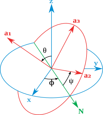
Figure 1.— Torque-free motion of a grain having three principal axes ${\bf a}_{1},{\bf a}_{2}$ and ${\bf a}_{3}$ in an inertial coordinate system with $\hat{\bf z}\|{\bf J}$ and $\hat{\bf x},~{}\hat{\bf y}\perp{\bf J}$ described by three Euler angles $\theta,\phi$ and $\psi$.

The dynamics of the irregular grain is more complicated than that of a disk-like grain. In addition to the precession of the axis of major inertia ${\bf a}_{1}$ about ${\bf J}$ as in the disk-like grain, the axis ${\bf a}_{1}$ wobbles rapidly, resulting in variations of the angle $\theta$ between ${\bf a}_{1}$ and ${\bf J}$ at a rate $\dot{\theta}$. Therefore, we expect the wobbling of the irregular grain can produce more frequency modes than those observed in the disk-like grain with $I_{2}=I_{3}$ (see HDL10).

To describe the torque-free motion of an irregular grain having a rotational energy $E_{\rm rot}$, we use conserved quantities, including the angular momentum ${\bf J}$, and a dimensionless parameter that characterizes the deviation of the grain rotational energy from its minimum value,

$$q=\frac{2I_{1}E_{\rm rot}}{J^{2}}.$$ (4)

Following Weingartner & Draine (2003), we define the total number of states $s$ in phase space for $q$ ranging from $1$ to $q$ as

$$s\equiv 1-\frac{2}{\pi}\int_{0}^{\psi_{1}}d\psi\left[\frac{I_{3}(I_{1}-I_{2}q)+I_{1}(I_{2}-I_{3})\cos^{2}\psi}{I_{3}(I_{1}-I_{2})+I_{1}(I_{2}-I_{3})\cos^{2}\psi}\right]^{1/2},~{}~{}~{}~{}$$ (5)

where

$$\psi_{1}=\cos^{-1}\left[\frac{I_{3}(I_{2}q-I_{1})}{I_{1}(I_{2}-I_{3})}\right]^{1/2},$$ (6)

for $q>q_{\rm sp}$ and $\psi_{1}=\pi/2$ for $q\leq q_{\rm sp}$, with $q_{\rm sp}\equiv I_{1}/I_{2}$ being the separatrix between the two regimes.

The instantaneous orientation of the grain in an inertial coordinate system is given by three Euler angles $\psi,\phi$ and $\theta$ (see Figure 1). The angular velocities are obtained by solving the Euler equations of motion. The torque-free motion of an irregular grain is treated in detail in Appendix A.

Briefly, the Euler equations give rise to two sets of solutions corresponding to $+$ and $-$ signs for $\omega_{i}$ with $i=1,2$ and $3$ (see Eqs A4-A6). It can be seen that for $q\leq q_{{\rm sp}}$, two rotation states $\pm$ correspond to $\omega_{1}>0$ and $\omega_{1}<0$, i.e., ${\bf a}_{1}\cdot{\bf J}>0$ and ${\bf a}_{1}\cdot{\bf J}<0$. Following Weingartner & Draine (2003), we refer to these rotation states as the positive flip state and negative flip state with respect to ${\bf a}_{1}$ (see also Hoang & Lazarian 2009a). For $q>q_{{\rm sp}}$, similarly, two rotation states correspond to $\omega_{3}>0$ and $\omega_{3}<0$, i.e., ${\bf a}_{3}\cdot{\bf J}<0$ and ${\bf a}_{3}\cdot{\bf J}>0$. These rotation sates are referred to as the positive and negative flip states with respect to ${\bf a}_{3}$.

3.2. Internal relaxation, thermal fluctuations and thermal flipping

3.2.1 Internal relaxation and thermal fluctuations

Internal relaxation (e.g. imperfect elasticity, Barnett relaxation; Purcell 1979; Lazarian & Efroimsky 1999) arises from the transfer of grain rotational energy to vibrational modes. For cold grains, this process tends to result in nearly perfect alignment of the grain axis of major inertia with the angular momentum. Naturally, if the grain has nonzero vibrational energy, energy can also be transferred from the vibrational modes into grain rotational energy (Jones & Spitzer 1969).

For an isolated grain, a small amount of energy gained from the vibrational modes results in fluctuations of the rotational energy $E_{{\rm rot}}$ when the grain angular momentum is conserved. Such fluctuations in $E_{{\rm rot}}$ result in fluctuations of $q$ and of the angle $\theta$ between ${\bf a}_{1}$ and ${\bf J}$ for an axisymmetric grain. For an irregular grain, the fluctuations in $E_{{\rm rot}}$ are described by fluctuations in $s(q)$ (see Eq. 5). Over time, the fluctuations in $E_{{\rm rot}}$ establish a local thermal equilibrium (LTE) at a rotational energy equilibrium temperature $T_{\rm rot}$.

3.2.2 Exchange of Vibrational-Rotational Energy

The Intramolecular Vibrational-Rotational Energy Transfer process (IVRET) due to imperfect elasticity occurs on a timescale $10^{-2}$ s, for a grain of a few Angstroms (Purcell 1979), which is shorter than the IR emission time. So, when the vibrational energy decreases due to IR emission, as long as the Vibrational-Rotational (V-R) energy exchange exists, interactions between vibrational and rotational systems maintain a thermal equilibrium, i.e., $T_{\rm rot}\approx T_{\rm vib}$. As a result, the LTE distribution function of rotational energy reads (hereafter VRE regime; see Lazarian & Roberge 1997):

$$f_{{\rm VRE}}(s,J)\propto{\rm exp}\left(-\frac{E_{\rm rot}}{k_{{\rm B}}T_{{\rm rot}}}\right)\approx{\rm exp}\left(-\frac{E_{\rm rot}}{k_{{\rm B}}T_{{\rm vib}}}\right).$$ (7)

The existence of V-R energy exchange depends on the rotational modes. In principle, the rotational energy can change in increments of $\hbar\omega$, with $\omega$ being the angular frequency of rotational modes. However, at low vibrational energy $E_{{\rm vib}}$, the vibrational mode spectrum is sparse, and there may not be available transitions with $\Delta E_{{\rm vib}}=\hbar\omega_{{\rm rot}}$. For the case ${\bf a}_{1}$ parallel to ${\bf J}$, the V-R energy exchange occurs only when the grain is hot just after absorption of a UV photon, because the grain rotating with ${\bf a}_{1}\|{\bf J}$ has only one rotational mode $\omega=\omega_{{\rm rot}}\equiv J/I_{1}$. As the grain cools down further, there is no available vibrational transition corresponding to an energy change $\hbar\omega_{{\rm rot}}$, and the V-R coupling ceases.

For disk-like or irregular grain, multiple rotational frequency modes are observed, and some modes correspond to energy $\hbar\omega>\hbar\omega_{{\rm rot}}$ (see Eq. 14 or Fig. 2). This may allow V-R energy exchange even when the vibrational energy is relatively low. Nevertheless, the energy separation between the vibrational ground state and the first vibrationally-excited state is large enough that V-R energy exchange is unlikely to take place after the PAH cools to the vibrational ground sate. The key, then, is to know the vibrational “temperature” of a cooling PAH at the time when V-R energy exchange ceases to be effective. Sironi & Draine (2009) estimated a decoupling temperature $T_{{\rm d}}=65$ K for a PAH with 200 C atoms.

In regions with the average starlight background, the mean time interval between absorptions of starlight photon will be $\sim 10^{6}$ s for a PAH containing 200 C atoms. Because the PAH will cool below $65$ K in $\sim 10^{3}$ s (see, e.g., Fig. 9 of Draine & Li 2001), V-R energy exchange will be suppressed most of the time, taking place only during $\sim 10^{3}$ s intervals following absorption of starlight photons. However, the $10^{6}$ s interval between photon absorptions is short compared to the timescale over which $J$ will change appreciably, and we will therefore approximate the V-R energy exchange process as continuous, even though it is episodic.

Substituting $E_{{\rm rot}}$ as a function of $J$ and $q$ from Equation (4) into Equation (7), the distribution function for the rotational energy becomes

$$f_{{\rm VRE}}(s,J)=A{\rm exp}\left(-\frac{q(s)J^{2}}{2I_{1}k_{{\rm B}}T_{{\rm vib}}}\right),$$ (8)

where $A$ is a normalization constant such that $\int_{0}^{1}f_{{\rm VRE}}(s,J)ds=1$.

Define a rotational temperature $T_{J}=J^{2}/2I_{1}k_{{\rm B}}$. Thus, the distribution for $q$ becomes $f_{{\rm VRE}}\propto{\rm exp}\left(-q(s)T_{J}/T_{{\rm vib}}\right)$. When $T_{J}\gg T_{{\rm vib}}$, the grain is suprathermally rotating, and ${\bf a}_{1}$ is aligned with ${\bf J}$. In contrast, when $T_{J}\ll T_{{\rm vib}}$, the grain rotates subthermally, and thermal fluctuations randomize the grain axes with respect to ${\bf J}$. For fixed angular momentum, the thermal fluctuations increase with $T_{{\rm vib}}$.

3.2.3 Thermal flipping

Transfer of energy between the vibrational and rotational modes due to dissipation or thermal fluctuations will cause $E_{{\rm rot}}$, and therefore $q$, to vary with time. If $q$ crosses the separatrix state $q=q_{{\rm sp}}$, the new flip state is effectively chosen randomly. Changes in $q$ can also result from external forcing (e.g., collisions with gas atoms or absorption/emission of radiation), that may change both $J$ and $E_{{\rm rot}}$. If the external torques are not “chiral”, then the changes in $q$ over time will result in equal probabilities of the two flip states. However, the chirality of the grain may lead to $q$-changing processes that depend not only on $q$, but also on which flip state the grain is in. The present treatment neglects any grain chirality.

4. Electric Dipole Emission from Grains of Irregular Shape

Below we investigate electric dipole emission arising from irregular grains. We first calculate emission power spectra arising from a torque-free rotating irregular grain. Then, we compute the spinning dust emissivity and compare the results with those from disk-like grains.

4.1. Power Spectrum

A torque-free rotating irregular grain can rotate either in the positive or negative flip state, and the treatment in this section is applicable for a general flip state. To find the electric dipole emission spectrum from such an isolated irregular grain, we follow the approach in HDL10. We first represent the dipole moment ¯ in an inertial coordinate system, and then compute its second derivative. We obtain

$$\ddot{{\hbox{\boldsym\char 22\relax}}}=\sum_{i=1}^{3}\mu_{i}\ddot{{\bf a}}_{i},$$ (9)

where $\mu_{i}$ are components of ¯ along principal axes ${\bf a}_{i}$, $\ddot{{\bf a}}_{i}$ are second derivative of ${\bf a}_{i}$ with respect to time, and $i=1,2$ and $3$.

The instantaneous emission power of the dipole moment is defined by

$$P_{\rm ed}(J,q,t)=\frac{2}{3c^{3}}\ddot{\hbox{\boldsym\char 22\relax}}^{2}.$$ (10)

The power spectrum is then obtained from the Fourier transform (FT) for the components of $\ddot{\hbox{\boldsym\char 22\relax}}$. For example, the amplitude of $\ddot{\mu}_{x}$ at the frequency $\nu_{k}$ is defined as

$$\ddot{\mu}_{x,k}=\int_{-\infty}^{+\infty}\ddot{\mu}_{x}(t){\rm exp}\left(-i2\pi\nu_{k}t\right)dt,$$ (11)

where $k$ denotes the frequency mode. The emission power at the positive frequency $\nu_{k}$ is given by

$$P_{{\rm ed},k}(J,q)=\frac{4}{3c^{3}}(\ddot{\mu}_{x,k}^{2}+\ddot{\mu}_{z,k}^{2}+\ddot{\mu}_{z,k}^{2}),$$ (12)

where the factor $2$ arises from the positive/negative frequency symmetry of the Fourier spectrum. To reduce the spectral leakage in the FT, we convolve the time function $\ddot{\hbox{\boldsym\char 22\relax}}$ with a Blackman-Harris window function (Harris 1978). The power spectrum needs to be corrected for the power loss due to the window function.

The total emission power from all frequency modes for a given $J$ and $q$ is then

$$P_{{\rm ed}}(J,q)=\sum_{k}P_{{\rm ed},k}(J,q)\equiv\frac{1}{T}\int_{0}^{T}dt\left(\frac{2}{3c^{3}}\ddot{\hbox{\boldsym\char 22\relax}}^{2}\right),~{}~{}~{}$$ (13)

where $T$ is the integration time.

Here we compute power spectra for case 1 ($\mu_{1}=\mu/\sqrt{3}$) of ¯ orientation, but our approach can be used straightforward for any orientation of ¯.

Figure 2 presents normalized power spectra (squared amplitude of Fourier transforms), $|{\rm FT}(\mu_{x,y})|^{2}/\max(|{\rm FT}(\mu_{x})|^{2})$ and $|{\rm FT}(\mu_{z})|^{2}/\max(|{\rm FT}(\mu_{x})|^{2})$ for the components $\ddot{\mu}_{x}$ (or $\ddot{\mu}_{y}$) and $\ddot{\mu}_{z}$, for a torque-free rotating irregular grain having the ratio of moments of inertia $I_{1}:I_{2}:I_{3}=1:0.6:0.5$ in the positive flip state with various $q$. Circles and triangles denote peaks of the power spectrum for components of $\ddot{\mu}_{x}$ (or $\ddot{\mu}_{y}$) and $\ddot{\mu}_{z}$, respectively.

Multiple frequency modes are observed in the power spectra of the irregular grain, but in Figure 2 we show only the modes with power no less than $10^{-3}$ the maximum value. Both positive and negative flip states have the same frequency modes.

For $q<I_{1}/I_{2}$, we found that power spectra for $\ddot{\mu}_{x}$ (or $\ddot{\mu}_{y}$) have angular frequency modes

$$\omega_{m}\approx\langle\dot{\phi}\rangle+m\langle|\dot{\psi}|\rangle,$$ (14)

where the bracket denotes the averaging value over time, and $m=0,\pm 1,\pm 2...$ denote the order of the mode. The frequency modes for $\ddot{\mu}_{z}$ are given by

$$\omega_{n}=n\langle|\dot{\psi}|\rangle,$$ (15)

where $n$ is integer and $n\geq 1$.

The above frequency modes are equivalent to results obtained from a quantum mechanical treatment. For the limiting case of an axisymmetric grain with $I_{1}>I_{2}=I_{3}$, the grain rotational Hamiltonian is $H=J^{2}/2I_{2}-J_{z}^{2}(I_{1}-I_{2})/(2I_{1}I_{2})$ where $J_{z}=J\cos\theta$ is the projection of ${\bf J}$ on the symmetry axis. From a quantitization, $J^{2}\rightarrow J(J+1)\hbar^{2}$ and $J_{z}\rightarrow K\hbar$ where $J$ and $K$ are quantum numbers for the angular momentum and its projection on the grain symmetry axis, the rotational energy is written as $E_{J,K}=J(J+1)\hbar^{2}/2I_{2}-K^{2}\hbar^{2}(I_{1}-I_{2})/(2I_{1}I_{2})$. For PAHs, $J$ is usually very large, so an emission mode arising from the transition from the energy level $E_{J,K}$ to $E_{J^{\prime},K^{\prime}}$ have frequency given by

$$\omega_{JJ^{\prime},KK^{\prime}}=\frac{1}{\hbar}\left(\frac{\partial E_{J,K}}{\partial J}\Delta J+\frac{\partial E_{J,K}}{\partial K}\Delta K\right),$$ (16)

where $\partial E_{J,K}/\partial J\approx(J\hbar^{2}/I_{2})=\hbar\dot{\phi}$ and $\partial E_{J,K}/\partial K=(K\hbar^{2}/I_{1}I_{2})(I_{1}-I_{2})=\hbar\dot{\psi}$. The selection rules for electric dipole transitions correspond to $\Delta J=0,~{}\pm 1$, and $\Delta K=0,~{}\pm 1$, so the total emission modes are $\omega_{JJ^{\prime},KK^{\prime}}=\dot{\phi},~{}\dot{\phi}\pm\dot{\psi}$ and $\dot{\psi}$, as found in HDL10. The rotational energy levels of asymmetric rotors are specified by three quantum numbers – the total angular momentum $J$ and two additional quantum numbers $K_{-1}$ and $K_{+1}$. Electric dipole transitions obey selection rules $\Delta J=0,\pm 1$, $\Delta K_{-1}=\pm 1,\pm 3$, and $\Delta K_{+1}=\pm 1,\pm 3$ (see, e.g., Townes & Schawlow 1955) . In the large $J$ limit, these selection rules will correspond to the modes of Equations (14) and (15).

For $q>I_{1}/I_{2}$, only the mode $m=0$ has angular frequency given by Equation (14).

In the following, the emission modes induced by the oscillation of $\mu_{x}$ or $\mu_{y}$, which lie in the $\hat{\bf x}\hat{\bf y}$ plane, perpendicular to ${\bf J}$, are called in-plane modes, and those induced by the oscillation of $\mu_{z}$ in the direction perpendicular to the $\hat{\bf x}\hat{\bf y}$ plane, are called out-of-plane modes. The order of mode is denoted by $m$ and $n$, respectively.

Figure 2 also shows that the emission power for out-of-plane modes $\omega_{n}$ is negligible compared to the power emitted by in-plane modes $\omega_{m}$.

The upper panel in Figure 3 shows the variation of the angular frequency of the dominant modes $m=0,\pm 1,\pm 2$ with $q$. The kink at $q=q_{\rm sp}=I_{1}/I_{2}$ in $\omega_{m}$ arises from the change of grain rotation state. For $q<q_{\rm sp}$, the frequency $\omega_{m=0}=\langle\dot{\phi}\rangle$ is almost constant, whereas it increases with $q$ to $\omega_{m=0}=J/I_{3}$ at $q=I_{1}/I_{3}$. The frequency of the mode $m=1$ also increases with $q$ for $q>q_{\rm sp}$. The increase of frequency for the two dominant modes $m=0$ and $1$ for $q>q_{\rm sp}$ can result in an increase of peak frequency of spinning dust spectrum. This issue will be addressed in the next section.

The middle panel in Figure 3 shows the emission power at the dominant frequency modes $|m|\leq 2$. For $q\sim 1$, most of emission comes from the mode $m=-1$. As $q$ increases, the mode $m=0$ becomes dominant.

The total emission power from all modes for irregular grains of different $I_{2}:I_{3}$ and $I_{1}:I_{2}=1:0.6$ is shown in the right panel.

Figure 2.— Normalized power spectrum of a torque-free rotating irregular grain with $I_{1}:I_{2}:I_{3}=1:0.6:0.5$ for different values of $q=1.05,1.60$ (i.e. $q<q_{\rm sp}\equiv I_{1}/I_{2}$) and $q=1.81>q_{\rm sp}$. The components of $|{\rm FT}(\ddot{\mu}_{x})|^{2}/\max(|{\rm FT}(\ddot{\mu}_{x})|^{2}))$ (or $|{\rm FT}(\ddot{\mu}_{y})|^{2}/\max(|{\rm FT}(\ddot{\mu}_{x})|^{2})$) are indicated by circles, while the components of $|{\rm FT}(\ddot{\mu}_{z})|^{2}/\max(|{\rm FT}(\ddot{\mu}_{x})|^{2})$ are indicated by triangles. Orders of in-plane modes $m$ and out-of-plane modes $n$ are indicated, and case 1 ($\mu_{1}=\mu/\sqrt{3}$) of ¯ orientation is assumed.

Figure 3.— Left: Angular frequency of in-plane modes as a function of $q$ for an irregular grain with $I_{1}:I_{2}:I_{3}=1:0.6:0.5$. The kink at $q=q_{\rm sp}\equiv I_{1}/I_{2}$ corresponds to the change from rotation around ${\bf a}_{1}$ to rotation around ${\bf a}_{3}$. Middle: Emission power radiating at frequency modes $\omega_{m}$ as a function of $q$. Right: Total emission power from all frequency modes as a function of $q$ for various ratios $I_{2}:I_{3}$ while $I_{1}:I_{2}=1:0.6$ is kept constant. Case 1 ($\mu_{1}=\mu/\sqrt{3}$) of ¯ orientation is considered.

We compute emission power spectra to infer $\omega_{k}$ and $P_{{\rm ed},k}$, as functions of $J$ and $q$, for various ratio of moments of inertia $I_{1}:I_{2}:I_{3}$. The obtained data will be used later to compute spinning dust emissivity.

4.2. Spinning Dust Emissivity

To calculate the spinning dust emissivity, the first step is to find the distribution function for grain angular momentum.

4.2.1 Angular Momentum Distribution Function

Following HDL10, to find the distribution function for the grain angular momentum ${\bf J}$, we solve Langevin equations describing the evolution of ${\bf J}$ in time in an inertial coordinate system. They read

$$dJ_{i}=A_{i}dt+\sqrt{B_{ii}}dq_{i},\mbox{~{}for~{}}i=\mbox{~{}x,~{}y,~{}z},$$ (17)

where $dq_{i}$ are random Gaussian variables with $\langle dq_{i}^{2}\rangle=dt$, $A_{i}=\langle{\Delta J_{i}}/{\Delta t}\rangle$ and $B_{ii}=\langle\left({\Delta J_{i}}\right)^{2}/{\Delta t}\rangle$ are damping and diffusion coefficients defined in the inertial coordinate system.

For an irregular grain, to simplify calculations, we adopt the $A_{i}$ and $B_{ii}$ for a disk-like grain obtained in HDL10. Following DL98b and HDL10, the disk-like grain has radius $R$ and thickness $L=3.35\,{\rm\AA}$, and the ratio of moments of inertia along and perpendicular to the grain symmetry axis $h=I_{\|}/I_{\perp}$. Thereby, the effect of nonaxisymmetry on $A_{i}$ and $B_{ii}$ is ignored, and we examine only the effect the wobbling resulting from the irregular shape has on the spinning dust emissivity.

In dimensionless units, ${\bf J}^{\prime}\equiv{\bf J}/I_{\|}\omega_{\rm T,\|}$ with $\omega_{\rm T,\|}\equiv\left(2k_{{\rm B}}T_{\,{\rm gas}}/I_{\|}\right)^{1/2}$ being the thermal angular velocity of the grain along the grain symmetry axis, and $t^{\prime}\equiv t/\tau_{\rm H,\|}$, Equation (17) becomes

$$dJ^{\prime}_{i}=A^{\prime}_{i}dt^{\prime}+\sqrt{B^{\prime}_{ii}}dq^{\prime}_{i},$$ (18)

where $\langle dq_{i}^{{}^{\prime}2}\rangle=dt^{\prime}$ and

$$A^{\prime}_{i} = -\frac{J^{\prime}_{i}}{\tau^{\prime}_{\,{\rm gas},{\rm eff}}}-\frac{2}{3}\frac{J_{i}^{{}^{\prime}3}}{\tau^{\prime}_{{\rm ed},{\rm eff}}},~{}~{}~{}~{}$$ (19)

$$B^{\prime}_{ii} = \frac{B_{ii}}{2I_{\|}k_{\rm B}T_{\,{\rm gas}}}\tau_{{\rm H},\|},$$ (20)

where

$$\tau^{\prime}_{\,{\rm gas},{\rm eff}} = \frac{\tau_{\,{\rm gas},{\rm eff}}}{\tau_{{\rm H},\|}}=\frac{F_{\rm tot,\|}^{-1}}{\cos^{2}\theta+\gamma_{{\rm H}}\sin^{2}\theta},$$ (21)

$$\gamma_{\rm H} = \frac{F_{\rm tot,\perp}\tau_{\rm H,\|}}{F_{\rm tot,\|}\tau_{\rm H,\perp}},$$ (22)

$$\tau^{\prime}_{{\rm ed},{\rm eff}} = \frac{\tau_{{\rm ed},{\rm eff}}}{\tau_{\rm H,\|}},~{}~{}~{}$$ (23)

where $\tau_{{\rm H},\|}$ and $\tau_{{\rm H},\perp}$ are rotational damping times due to gas of purely hydrogen atom for rotation along parallel and perpendicular direction to the grain symmetry axis ${\bf a}_{1}$, $\tau_{{\rm ed},{\rm eff}}$ is the effective damping time due to electric dipole emission (see Appendix B), $\theta$ is the angle between ${\bf a}_{1}$ and ${\bf J}$, and $F_{\rm tot,\|}$ and $F_{\rm tot,\perp}$ are total damping coefficients parallel and perpendicular to ${\bf a}_{1}$ (see HDL10).

At each time step, the angular momentum $J_{i}$ obtained from LEs is recorded and later used to find the distribution function $f_{J}$ with normalization $\int_{0}^{\infty}f_{J}dJ=1$.

4.2.2 Emissivity from Irregular Grains

As discussed in §4.1, an irregular grain rotating with a given angular momentum $J$ radiates at frequency modes $\omega_{k}\equiv\omega_{m}$ with $m=0,\pm 1,\pm 2...$ and $\omega_{k}\equiv\omega_{n}$ with $n=1,2,3...$ (see Eqs 14 and 15). For simplicity, we define the former as $\omega_{{\rm m}_{i}}$ and the latter as $\omega_{{\rm n}_{i}}$ where $i$ indicates the value for $m$ and $n$. These frequency modes depend on the parameter $q(s)$, which is determined by the internal thermal fluctuations within the grain.

To find the emissivity at an observation frequency $\nu=\omega/2\pi$, we need to know how much emission each mode $\omega_{k}$ contributes to the observation frequency $\nu$.

Consider an irregular grain rotating with the angular momentum $J$, the probability of finding the emission at the angular frequency $\omega$ depends on the probability of finding the value $\omega$ such that

$$pdf(\omega|J)d\omega=f_{{\rm VRE}}(s,J)ds=A{\rm exp}\left(-\frac{q(s)J^{2}}{2I_{1}k_{{\rm B}}T_{{\rm vib}}}\right)ds,~{}~{}~{}~{}~{}$$ (24)

where we assumed the VRE regime with $f_{{\rm VRE}}$ given by Equation (8).

For the mode $\omega\equiv\omega_{k}(s)$, from Equation (24) we can derive

$$pdf_{k}(\omega|J)=\left(\frac{\partial\omega_{k}}{\partial s}\right)^{-1}f_{{\rm VRE}}(s,J).$$ (25)

The emissivity from the mode $k$ is calculated as

$$j_{\nu,k}^{a} = \frac{1}{4\pi}\int_{J_{l}}^{J_{u}}P_{{\rm ed},k}(J,q_{\leq})f_{J}(J)pdf_{k}(\omega|J)2\pi~{}dJ$$ (26)

$$+\frac{1}{4\pi}\int_{J_{l}}^{J_{u}}P_{{\rm ed},k}(J,q_{>})f_{J}(J)pdf_{k}(\omega|J)2\pi~{}dJ,~{}~{}~{}~{}~{}$$

where $q_{\leq}$ and $q_{>}$ denote $q\leq q_{{\rm sp}}$ and $q>q_{{\rm sp}}$, respectively; $J_{l}$ and $J_{u}$ are lower and upper limits for $J$ corresponding to a given angular frequency $\omega_{k}(J,q)=\omega$, and $2\pi$ appears due to the change of variable from $\nu$ to $\omega$.

Emissivity by a grain of size $a$ at the observation frequency $\nu$ arising from all emission modes is then

$$j_{\nu}^{a} \equiv \sum_{k}j_{\nu,k}^{a}.$$ (27)

Consider for example the emission mode $k\equiv{\rm m}_{0}$. For the case $I_{2}$ slightly larger than $I_{3}$, this mode has the angular frequency $\omega_{{\rm m}_{0}}=\langle\dot{\phi}\rangle=(J/I_{1})q_{0}$ with $q_{0}$ obtained from calculation of $\omega_{{\rm m}_{0}}$, is independent on $q$ for $q<q_{{\rm sp}}$. As a result

$$pdf_{{\rm m}_{0}}(\omega|J)=\delta\left(\omega-(J/I_{1})q_{0}\right).$$ (28)

Thus, the first term of Equation (26), denoted by $j_{\nu,{\rm m}_{0},\leq}^{a}$, is rewritten as

$$j_{\nu,{\rm m}_{0},\leq}^{a} = \frac{1}{2}\int_{J_{l}}^{J_{u}}P_{{\rm ed},{\rm m}_{0}}(J,q_{\leq})f_{J}(J)\delta\left(\omega-(J/I_{1})q_{0}\right)dJ,$$ (29)

$$= \frac{1}{2}\frac{I_{1}f_{J}(J_{0})}{q_{0}}P_{{\rm ed},{\rm m}_{0}}(J_{0},q(s)),$$

where $J_{0}=I_{1}\omega/q_{0}$, and the value of $q(s)$ remains to be determined.

For $q>q_{{\rm sp}}$, $\langle\dot{\phi}\rangle$ is a function of $q$. Hence, the emissivity (26) for the mode $k\equiv{\rm m}_{0}$ becomes

$$j_{\nu,{\rm m}_{0}}^{a} = \frac{1}{2}\frac{I_{1}f_{J}(J_{0})}{q_{0}}\int_{0}^{s_{{\rm sp}}}dsP_{{\rm ed},{\rm m}_{0}}(J_{0},q(s))f_{{\rm VRE}}(J_{0},s)$$ (30)

$$+\frac{1}{2}\int_{J_{l}}^{J_{u}}P_{{\rm ed},{\rm m}_{0}}(J,q_{>})f_{J}(J)pdf_{{\rm m}_{0}}(\omega|J)dJ,~{}~{}~{}~{}~{}$$

where $s_{{\rm sp}}$ is the value of $s$ corresponding to $q=q_{{\rm sp}}$, and the term $P_{{\rm ed},{\rm m}_{0}}(J_{0},q(s))$ in Equation (29) has been replaced by its average value over the internal thermal distribution $f_{{\rm VRE}}$.

The emissivity per H is obtained by integrating $j_{\nu}^{a}$ over the grain size distribution:

$${j_{\nu}\over n_{\rm H}}={1\over n_{\rm H}}\int_{a_{\rm min}}^{a_{\rm max}}da{dn\over da}j_{\nu}^{a}~{},$$ (31)

where $j_{\nu}^{a}$ is given by Equation (26).

4.2.3 Emissivity from Disk-like Grains

HDL10 showed that a disk-like grain with an angular momentum ${\bf J}$ radiates at frequency modes

$$\omega_{{\rm m}_{i}} \equiv \dot{\phi}+i\dot{\psi}=\frac{J}{I_{\|}}\left[h+i(1-h)\cos\theta\right],$$ (32)

$$\omega_{n_{1}} \equiv \dot{\psi}=\frac{J}{I_{\|}}(1-h)\cos\theta,$$ (33)

where $i=0$ and $\pm 1$.

The emission power of these modes are given by following analytical forms (HDL10; Silsbee et al. 2011):

$$P_{\omega_{{\rm m}_{0}}} = \frac{2\mu_{\|}^{2}}{3c^{3}}\omega_{{\rm m}_{0}}^{4}\sin^{2}\theta,$$ (34)

$$P_{\omega_{{\rm m}_{\pm 1}}} = \frac{\mu_{\perp}^{2}}{6c^{3}}\omega_{{\rm m}_{\pm 1}}^{4}(1\pm\cos\theta)^{2},$$ (35)

$$P_{\omega_{{\rm n}_{1}}} = \frac{2\mu_{\perp}^{2}}{3c^{3}}\omega_{{\rm n}_{1}}^{4}\sin^{2}\theta.$$ (36)

For the disk-like grain, from Equation (5), we obtain the number of state in phase space $s$ for $q$ spanning from $1-q$:

$$s=1-\left(\frac{h-q}{h-1}\right)^{1/2}=1-\cos\theta,$$ (37)

where $q=1+(h-1)\sin^{2}\theta$ has been used. Thus, for an arbitrary mode with frequency $\omega_{k}$, we obtain

$$pdf_{k}(\omega|J)d\omega=f_{{\rm VRE}}(s,J)ds=f_{{\rm VRE}}(\theta,J)\sin\theta d\theta.~{}~{}~{}$$ (38)

Taking use of $\omega=\omega_{k}(J,\theta)$, we derive

$$pdf_{k}(\omega|J)=f_{{\rm VRE}}(\theta,J)\left(\frac{\partial\omega_{k}}{\partial\theta}\right)^{-1}\sin\theta.$$ (39)

Therefore, by substituting Equations (34)-(36) in Equation (26), the emissivity at the observation frequency $\nu=\omega/(2\pi)$ from a disk-like grain of size $a$ is now given by

$$j_{\nu}^{a} \equiv \frac{1}{2}\frac{f_{J}(I_{\|}\omega/h)}{h}\frac{2\mu_{\|}^{2}}{3c^{3}}\omega^{4}\langle\sin^{2}\theta\rangle$$ (40)

$$+\frac{1}{2}\frac{\mu_{\perp}^{2}}{6c^{3}}\omega^{4}\int_{J_{l}}^{J_{u}}pdf_{{\rm m}_{1}}(\omega|J)f_{J}(J)dJ$$

$$+\frac{1}{2}\frac{\mu_{\perp}^{2}}{6c^{3}}\omega^{4}\int_{J_{l}}^{J_{u}}pdf_{{\rm m}_{-1}}(\omega|J)f_{J}(J)dJ$$

$$+\frac{1}{2}\frac{\mu_{\perp}^{2}}{3c^{3}}\omega^{4}\int_{J_{l}}^{J_{u}}pdf_{{\rm n}_{1}}(\omega|J)f_{J}(J)dJ,$$

where $pdf_{{\rm m}_{\pm 1}}$ and $pdf_{{\rm n}_{1}}$ are easily derived by using Equation (39) for $\omega_{{\rm m}_{\pm 1}}$ and $\omega_{{\rm n}_{1}}$, and $J_{l}=I_{\|}\omega/(2h-1)$ and $J_{u}=I_{\|}\omega$ for $m_{\pm 1}$ mode, and $J_{l}=I_{\|}\omega/(h-1)$ and $J_{u}=\infty$ for $n_{1}$ mode (see Eqs 32 and 33) .

As in HDL10, we also consider the regime without internal relaxation. Then, the distribution function $f_{{\rm VRE}}(\theta,J)$ is replaced by a Maxwellian distribution (hereafter Mw regime):

$$f_{\rm Mw}(\theta)=\frac{h}{4\pi}\frac{1}{\left(\cos^{2}\theta+h\sin^{2}\theta\right)^{3/2}}.$$ (41)

For symmetric rotors ($h=1$), the distribution function for $\theta$ is isotropic:

$$f_{\rm iso}(\theta)=\frac{1}{4\pi},$$ (42)

satisfying the normalization condition $\int_{0}^{\pi}f_{\rm iso}(\theta)2\pi\sin\theta d\theta=1$

4.3. Results

In this section, we present results for spinning dust emissivity from grains of irregular shape obtained using the method in Section 4.2.

4.3.1 A Simple Model of Irregular Grain

We assume that smallest grains of size $a\leq a_{2}=6\,{\rm\AA}$, have planar shape, and larger grains are spherical. To compare with emission from the disk-like grains, we consider the simplest case of the irregular shape in which the circular cross-section of the disk-like grain is changed to elliptical cross-section. We are interested in the emission of two PAHs with the same mass $M$ and thickness $L$, therefore, the length of the semi-axes of elliptical disk is constrained by

$$M=\pi R^{2}L=\pi b_{2}b_{3}L,$$ (43)

where $R=(4a^{3}/3L)^{1/2}$ is the radius of the disk-like grain, $b_{2}$ and $b_{3}$ are the length of semi-axes ${\bf a}_{2}$ and ${\bf a}_{3}$, and $b_{1}=L$ is kept constant. Assuming that the circular disk is compressed by a factor $\alpha\leq 1$ along ${\bf a}_{2}$, then Equation (43) yields

$$b_{2}=\alpha R,~{}~{}b_{3}=\alpha^{-1}R.$$ (44)

Denote the parameter $\eta\equiv b_{3}/b_{2}=\alpha^{-2}$, then the degree of grain shape irregularity is completely characterized by $\eta$.

The moments of inertia along the principal axes for the irregular grain are

$$I_{1}=\frac{M}{4}\left(b_{2}^{2}+b_{3}^{2}\right)=\frac{I_{\|}}{2}\left(\eta+\eta^{-1}\right),$$ (45)

where $I_{\|}$ is the moment of inertia for the disk-like grain. The ratios of moment of inertia read

$$\frac{I_{1}}{I_{2}}=\frac{3\left(\eta+\eta^{-1}\right)}{(L/R)^{2}+3\eta},$$ (46)

$$\frac{I_{2}}{I_{3}}=\frac{(L/R)^{2}+3\eta}{(L/R)^{2}+3\eta^{-1}},$$ (47)

For each grain size $a$, the parameter $\eta$ is increased from $\eta=1$ to $\eta=\eta_{\max}$. However, $\eta_{\max}$ is constrained by the fact that the shortest axis ${\bf a}_{2}$ should not be shorter than the grain thickness $L$. We below assume conservatively $\eta_{\max}\sim 3/2$.

4.3.2 Rotational Emission Spectrum

Although irregular grains radiate in large number of frequency modes, we take into account only the dominant modes with order $|m|\leq 2$, and disregard the modes that contribute less than $\sim 0.5\%$ to the total emission. We also assume that grains smaller than $a_{2}$ have a fixed vibrational temperature $T_{{\rm vib}}$, and that for the instantaneous value of $J$ the rotational energy has a probability distribution $f_{{\rm VRE}}$ (i.e. VRE regime).

We adopt the grain size distribution $dn/da$ from Draine & Li (2007) with the total to selective extinction $R_{\rm V}=3.1$ and the total carbon abundance per hydrogen nucleus $b_{\rm C}=5.5\times 10^{-5}$ in carbonaceous grains with $a_{\min}=3.55\,{\rm\AA}$ and $a_{\max}=100\,{\rm\AA}$.

The spinning dust emissivity is calculated for a so-called model A (similar to DL98b; HDL10), in which $25\%$ of grains have the electric dipole moment parameter $\beta=2\beta_{0}$, $50\%$ have $\beta=\beta_{0}$ and $25\%$ have $\beta=0.5\beta_{0}$ with $\beta_{0}=0.4$ D. In the rest of the paper, the notation model A is omitted, unless stated otherwise.

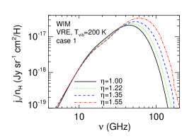
Figure 4.— Emissivity per H from irregular grains of different degree of irregularity $\eta=b_{3}/b_{2}$ with $T_{{\rm vib}}=20$, $60$ and $200$ K for case 1 ($\mu_{1}=\mu/\sqrt{3}$) of dipole moment orientation in the WIM. The emission spectrum shifts to higher frequency as $\eta$ decreases. The grain mass is held fixed as $\eta$ changes.

Figure 4 shows the spinning dust spectra for different degree of irregularity $\eta$ and various dust temperature $T_{{\rm vib}}$ in the WIM. The emission spectrum for a given $T_{{\rm vib}}$ shifts to higher frequency as $\eta$ decreases (i.e. the degree of grain irregularity increases), but their spectral profiles remain similar.

Figure 5.— The variation of peak frequency (left) and peak emissivity (right) as a function of the length ratio of semi-axes of elliptical disk, $\eta=b_{3}/b_{2}$ for various $T_{{\rm vib}}$ and case 1 ($\mu_{1}=\mu/\sqrt{3}$) of ¯ orientation in the WIM conditions. Both $\nu_{{\rm peak}}$ and $j_{{\rm peak}}$ increase fast with $\eta$ for $T_{{\rm vib}}\geq 60~{}{\rm K}$, but they changes slightly at $T_{{\rm vib}}=20~{}{\rm K}$

.

Figure 6.— Similar to Fig. 5, but for case 2 ($\mu_{1}=0$) of ¯ orientation. $\nu_{{\rm peak}}$ increases with $\eta$ for $T_{{\rm vib}}>20~{}{\rm K}$. $j_{{\rm peak}}$ increase with $\eta$ for $T_{{\rm vib}}\geq 100~{}{\rm K}$. For $T_{{\rm vib}}<60~{}K$, $j_{{\rm peak}}$ increases slightly to $\eta\sim 1.23$ and then drops.

To see more clearly the effect of grain shape irregularity, in Figure 5, we show the variation of peak frequency $\nu_{{\rm peak}}$ and peak emissivity $j_{{\rm peak}}$ as a function of $\eta$ for different $T_{{\rm vib}}$ and for case 1 ($\mu_{1}=\mu/\sqrt{3}$) of ¯ orientation for the WIM.

For low $T_{{\rm vib}}$ (i.e. $T_{{\rm vib}}=20~{}{\rm K}$), $\nu_{{\rm peak}}$ increases slowly with $\eta$, while $j_{{\rm peak}}$ varies slightly. As $T_{{\rm vib}}$ increases, both $\nu_{{\rm peak}}$ and $j_{{\rm peak}}$ increase rapidly with $\eta$, but the former increases faster.

Figure 6 shows the results for case 2 ($\mu_{1}=0$) of ¯ orientation. Similar to case 1, $\nu_{{\rm peak}}$ increases with $\eta$ for $T_{{\rm vib}}\geq 60~{}{\rm K}$, but changes rather little for $T_{{\rm vib}}=20~{}{\rm K}$. The variation of $j_{{\rm peak}}$ with $\eta$ is more complicated. For $T_{{\rm vib}}\leq 60~{}{\rm K}$, it increases first to $\eta\sim 1.23$, and then drops as $\eta$ increases.

5. Spinning Dust Spectrum: exploring parameter space

Below we explore parameter space by varying dust temperature, the lower grain size cutoff, the grain dipole moment, and the gas density. Our results from previous section indicate that the spinning dust spectrum from grains of irregular shape is shifted in general to higher frequency, relative to that from disk-like grains, but their spectral profile remains similar. Therefore, it is sufficient to explore parameter space of spinning dust for disk-like grains, extrapolating to irregular grains using our results from the previous section. Spinning dust emissivity is then calculated using Equation (31) in which $j_{\nu}^{a}$ is given by Equation (40).

5.1. Effect of internal thermal fluctuations

In this section, we account for the fluctuations of the dust temperature in smallest grains.

Let $T_{{\rm d}}$ be the decoupling temperature for the V-R energy exchange. For $T_{{\rm vib}}>T_{{\rm d}}$, the V-R energy exchange is efficient, and $T_{{\rm rot}}\approx T_{{\rm vib}}$. For the instantaneous value of $J$ the rotational energy has a probability distribution (8) determined by V-R energy exchange (the VRE regime). For $T_{{\rm vib}}<T_{{\rm d}}$, no V-R energy exchange exists. The rotational emissivity averaged over temperature fluctuations for a fixed grain size reads

$$\langle j_{\nu}^{a}\rangle_{T} = \int j_{\nu}^{a}(T_{{\rm vib}}>T_{{\rm d}})\frac{dP}{dT_{{\rm vib}}}dT_{{\rm vib}}$$ (48)

$$+\int j_{\nu}^{a}(T_{{\rm rot}}\leq T_{{\rm d}})P_{0}\delta(T_{{\rm rot}}-T_{{\rm d}})dT_{{\rm rot}},$$

where

$$P_{0}=\int_{0}^{T_{{\rm d}}}\frac{dP}{dT_{{\rm vib}}}dT_{{\rm vib}},$$ (49)

is the probability of the grain having $T_{{\rm vib}}\leq T_{{\rm d}}$, and $dP/dT$ is the probability for the grain having temperature in $T,T+dT$.

Figure 7 shows spinning dust spectra averaged over temperature distribution, $\langle j_{\nu}(T_{{\rm d}})\rangle_{T}$, for various decoupling temperature $T_{{\rm d}}$ compared to spectra for grains having a single vibrational temperature $T_{{\rm vib}}=T_{{\rm d}}$, denoted by $j_{\nu}(T_{{\rm vib}}=T_{{\rm d}})$. For low $T_{{\rm d}}\leq 70~{}{\rm K}$, the averaged emissivity $\langle j_{\nu}(T_{{\rm d}})\rangle_{T}$ is larger than $j_{\nu}(T_{{\rm vib}}=T_{{\rm d}})$, but the difference between $j_{\nu}(T_{{\rm vib}}=T_{{\rm d}})$ and $\langle j_{\nu}(T_{{\rm d}})\rangle_{T}$ decreases as $T_{{\rm d}}$ increases.

For $T_{{\rm d}}=60$ K, Figure 7 shows that $\langle j_{\nu}(T_{{\rm d}})\rangle_{T}$ is approximate to $j_{\nu}(T_{{\rm vib}}=T_{{\rm d}})$ with the difference less than a few percent. In the rest of the paper, we adopt a conservative value $T_{{\rm d}}=60$ K and calculate the spinning dust emissivity assuming that all grains have a single temperature $T_{{\rm d}}$.

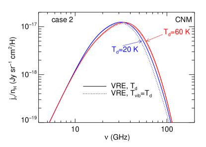
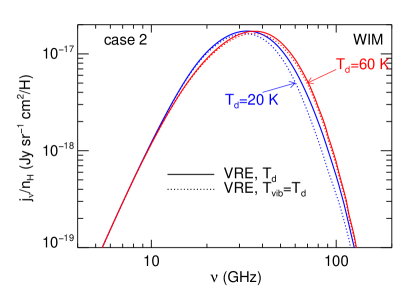
Figure 7.— Emissivity per H for case 2 ($\mu_{1}=0$) of the ¯ orientation and for the CNM and WIM. Solid and dotted lines are emissivity spectra averaged over temperature distribution, $\langle j_{\nu}(T_{{\rm d}})\rangle_{T}$, and spectra for grains having $T_{{\rm vib}}=T_{{\rm d}}$, $j_{\nu}(T_{{\rm vib}}=T_{{\rm d}})$, respectively. Two values $T_{{\rm d}}=20$ and $60~{}{\rm K}$ are chosen for illustration.

5.2. Minimum size $a_{\min}$

The spinning dust emission spectrum is sensitive to the population of smallest dust grains, and its peak frequency is mostly determined by the smallest grains. When $a_{\min}$ is increased, the peak frequency $\nu_{{\rm peak}}$ decreases accordingly.

Figure 8 shows the variation of $\nu_{{\rm peak}}$ as a function of $a_{\min}$ for various environments, and case 2 ($\mu_{1}=0$) of ¯ orientation and VRE regime ($T_{{\rm d}}=60~{}{\rm K}$). As expected, $\nu_{{\rm peak}}$ decreases generically with $a_{\min}$ increasing.

Figure 8.— Decrease of the peak frequency $\nu_{{\rm peak}}$ of spinning dust spectrum with the lower cutoff of the grain size distribution $a_{\min}$ for various environment conditions.

5.3. Effect of electric dipole moment

5.3.1 Variation of orientation of electric dipole moment

Silsbee et al. (2011) found that the total emission power $P_{{\rm ed}}$ and the peak frequency are rather insensitive to the orientation of the electric dipole moment. That stems from their calculations assuming no internal relaxation (i.e. $T_{{\rm vib}}\rightarrow\infty$), so that the angle $\theta$ is drawn from a isotropic distribution function $f_{\rm iso}$. Below we study the variation of emissivity $j_{\nu}$ with the orientation of dipole accounting for the internal relaxation.

To investigate the variation of $j_{\nu}$ with the orientation of ¯, in addition to case 1 ($\mu_{1}=\mu/\sqrt{3}$) and case 2 ($\mu_{1}=0$) of ¯ orientation, we consider values of $\mu_{\perp}^{2}/\mu^{2}$ between 2/3 (case 1) and 1 (case 2). We also consider the regime of fast internal relaxation (VRE) and without internal relaxation (Mw and iso). Model A for the distribution of electric dipole moment is adopted.

Figure 9 shows the variation of $\nu_{{\rm peak}}$ (upper panel) and $j_{{\rm peak}}$ (lower panel) of spinning dust spectrum with $\mu_{\perp}^{2}/\mu^{2}$. It can be seen that for the Mw and iso $f(\theta)$, $\nu_{{\rm peak}}$ changes rather slowly with $\mu_{\perp}^{2}/\mu^{2}$, with somewhat larger variation found in the VRE regime. The peak emissivity for all regimes exhibits similar trend that decreases with increasing $\mu_{\perp}^{2}/\mu^{2}$, though such a decrease is only $\sim 10\%$ when ¯ orientation changes from case 1 ($\mu_{1}=\mu/\sqrt{3}$) to case 2 ($\mu_{1}=0$).

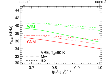
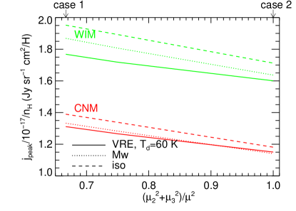
Figure 9.— Variation of the peak frequency $\nu_{{\rm peak}}$ (upper) and peak emissivity (lower) with ¯ orientation ($(\mu_{2}^{2}+\mu_{3}^{2})/\mu^{2}$) for VRE, Mw and iso regimes. $\nu_{{\rm peak}}$ for the VRE regime decreases faster than that for the Mw and iso regimes as ¯ orientation changes from case 1 ($\mu_{1}=\mu/\sqrt{3}$) to case 2 ($\mu_{1}=0$), but the decrease is within $10\%$.

5.3.2 Variation of distribution of electric dipole moment

Our standard model (model A, see Table 1) assumed grains of a given size $a$ to have three values of dipole moment, $\beta=\beta_{0},~{}\beta_{0}/2$ and $2\beta_{0}$ with $\beta_{0}=0.4~{}{\rm D}$, appearing in Equation (2).

Here we examine the possibility of considerable variation in the dipole moment per grain, by considering a model (model B) in which $40\%$ of grains have dipole moment parameter $\beta=\beta_{0}$; $15\%$ have $\beta=2\beta_{0}$ and $\beta_{0}/2$; $10\%$ have $\beta=4\beta_{0}$ and $\beta_{0}/4$; and $5\%$ have $\beta=8\beta_{0}$ and $\beta_{0}/8$. Emissivity per H for this model is compared with the typical model A in Figure 10.

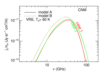
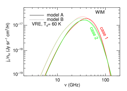
Figure 10.— Emissivity per H for the CNM (upper) and WIM (lower) for model A and B of dipole moment distribution and for case 1 ($\mu_{1}=\mu/\sqrt{3}$) and case 2 ($\mu_{1}=0$) of ¯ orientation and for the VRE ($T_{{\rm d}}=60~{}{\rm K}$) regime.

Figure 10 shows emission spectra for model A and B in cases 1 ($\mu_{1}=\mu/\sqrt{3}$) and 2 ($\mu_{1}=0$) of ¯ orientation, for the CNM and WIM. Results for the VRE ($T_{{\rm d}}=60$ K) regime are presented. The peak frequency from model B is lower than for model A, but model B has a higher peak emissivity. The larger value of $\langle\beta^{2}\rangle=3.12\beta_{0}^{2}$ in model B leads to stronger electric dipole emission but also stronger rotational damping.

5.4. Variation of values of dipole moment and gas density

Here we assume that all physical parameters are constant, including gas temperature and dust temperature. Only the value of characteristic dipole moment $\beta_{0}$ and gas density $n_{{\rm H}}$ are varied in calculations. We run LE simulations for $16$ values of $\beta_{0}$ from $0.05-3.2$ D, and 32 values of $n_{{\rm H}}$ from $10^{-2}-1\,{\rm cm}^{-3}$ for the WIM and from $1-100\,{\rm cm}^{-3}$ for the CNM. For a given value of $\beta_{0}$, the gaseous rotational damping time and the damping and excitation coefficient from infrared emission vary with the gas density $n_{{\rm H}}$ as

$$\tau_{{\rm H}} = \tau_{{\rm H}}(\overline{n}_{{\rm H}})\frac{\overline{n}_{{\rm H}}}{n_{{\rm H}}},$$ (50)

$$F_{{\rm IR}} = F_{{\rm IR}}(\overline{n}_{{\rm H}})\frac{\overline{n}_{{\rm H}}}{n_{{\rm H}}},~{}~{}~{}G_{{\rm IR}}=G_{{\rm IR}}(\overline{n}_{{\rm H}})\frac{\overline{n}_{{\rm H}}}{n_{{\rm H}}},$$ (51)

where $\overline{n}_{{\rm H}}$ is the typical gas density given in Table 2. Other rotational damping and excitation coefficients are independent of gas density.

The obtained distribution function for grain angular momentum is used to calculate spinning dust emissivity as functions of $\beta_{0}$ and $n_{{\rm H}}$ (see Sec. 4.2.3).

Figure 11 shows the contour of peak frequency $\nu_{{\rm peak}}$ and peak emissivity $j_{{\rm peak}}$ in the plane of $n_{{\rm H}},\beta_{0}$ for case 2 ($\mu_{1}=0$) of ¯ orientation in the CNM and WIM and for the VRE regime with $T_{{\rm d}}=60~{}{\rm K}$. For a given $\beta_{0}$, both $\nu_{{\rm peak}}$ and $j_{{\rm peak}}$ increase with $n_{{\rm H}}$ due to the increase of collisional excitation with $n_{{\rm H}}$. For a given $n_{{\rm H}}$, as $\beta_{0}$ increases, $\nu_{{\rm peak}}$ decreases, but $j_{{\rm peak}}$ increases. That is because as $\beta_{0}$ increases, electric dipole damping rate increases, which results in lower rotational rate of grains. Meanwhile, the emissivity increases with $\beta_{0}$ as $\beta_{0}^{2}$.

The results ($\nu_{{\rm peak}}$ and $j_{{\rm peak}}$) for the Mw regime are slightly larger than those for the former one due to the lack of internal relaxation.

From Figure 11 it can be seen that the amplitude of variation of $\nu_{{\rm peak}}$ and $j_{{\rm peak}}$ as functions of $n_{{\rm H}}$ and $\beta_{0}$ is very large. Thus, for a fixed grain size distribution, $n_{{\rm H}}$ and $\beta_{0}$ are the most important parameters in characterizing the spinning dust emission.

Figure 11.— Contour of peak frequency and peak emissivity in the plane of $n_{{\rm H}}$ and $\beta_{0}$ for the CNM (upper) and the WIM (lower), for the VRE ($T_{{\rm d}}=60$ K) regime. Case 2 ($\mu_{1}=0$) of ¯ orientation is considered. Peak frequency increases with $n_{{\rm H}}$ but decreases with $\beta_{0}$. Emissivity increases with both $n_{{\rm H}}$ and $\beta_{0}$.

6. Effect of Turbulence on Spinning Dust Spectrum

Turbulence is present at all scales of astrophysical systems (see Armstrong et al. 1995; Chepurnov & Lazarian 2010). The effects of turbulence on many astrophysical phenomena, e.g. star formation, cosmic rays transport and acceleration, have been widely studied. In the context of electric dipole emission from spinning dust, compressible turbulence will produce density variations that can affect grain charging, rotational excitation, and damping. We expect enhancement of spinning dust emissivity per particle from denser clumps, with an increase in the emission integrated along a line of sight. This issue is quantified in the following. For simplicity, we disregard the effect of turbulence on the grain charging.

6.1. Numerical Simulations of MHD turbulence

Gas density fluctuations in a turbulent medium is generated from Magneto-hydromagnetic (MHD) simulations. The sonic and Alfvenic Mach number are defined as usual $M_{\rm s}=\langle\frac{\delta V}{c_{s}}\rangle$, $M_{\rm A}=\langle\frac{\delta V}{v_{\rm A}}\rangle$ with $\delta V$ are amplitude for injection velocity, $c_{s}$ and $v_{\rm A}=B_{0}/\sqrt{4\pi\rho}$ are sound speed and Alfvenic speed.

The simulations are performed by solving the set of non-ideal MHD equations, in conservative form:

$$\frac{\partial\rho}{\partial t}+\mathbf{\nabla}\cdot(\rho{\bf v})=0,$$ (52)

$$\frac{\partial\rho{\bf v}}{\partial t}+\mathbf{\nabla}\cdot\left[\rho{\bf vv}+\left(p+\frac{B^{2}}{8\pi}\right){\bf I}-\frac{1}{4\pi}{\bf BB}\right]=\rho{\bf f},$$ (53)

$$\frac{\partial\mathbf{B}}{\partial t}-\mathbf{\nabla\times(v\times B)}=0,$$ (54)

with $\mathbf{\nabla\cdot B}=0$, where $\rho$, ${\bf v}$ and $p$ are the plasma density, velocity and pressure, respectively, ${\bf I}$ is the diagonal unit tensor, ${\bf B}$ is the magnetic field, and ${\bf f}$ represents the external acceleration source, responsible for the turbulence injection. Under this assumption, the set of equations is closed by an isothermal equation of state $p=c_{s}^{2}\rho$. The equations are solved using a second-order-accurate and non-oscillatory MHD code described in detail in Cho & Lazarian (2003). Parameters for the models of MHD simulations are shown in Table 3, including the sonic Mach number $M_{\rm s}$ and Alfvenic Mach number $M_{\rm A}$.

Table 3 Models of $512^{3}$ MHD simulations

Model	$M_{\,{\rm s}}$	$M_{\rm A}$	$v_{A}/c_{s}$	$\langle\rho^{2}\rangle/\langle\rho\rangle^{2}$
$1$	2.0	0.7	2.9	1.7
$2$	4.4	0.7	6.3	2.1
$3$	7.0	0.7	10	3.0

6.2. Results: influence of Gas Density Fluctuations

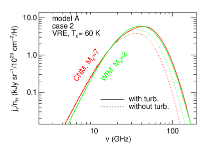
Figure 12.— Spinning dust emissivity per H in the presence of compressible turbulence with sonic Mach number $M_{\rm s}=2$ and $7$, compared to that from constant gas density $n_{{\rm H}}=\overline{n}_{{\rm H}}$ for the CNM (red) and WIM (green). The peak emissivity is increased, and the spectrum is shifted to higher frequency due to compressible turbulence. Case 2 ($\mu_{1}=0$) of ¯ orientation is considered

In a medium with density fluctuations, the effective emissivity is

$$\langle j_{\nu}\rangle=\int_{0}^{1}f(x)j_{\nu}(x\langle\rho\rangle)dx,$$ (55)

where $f(x)dx$ is the fraction of the mass with $\rho/\langle\rho\rangle\in(x,x+dx)$. We use compression distributions $f(x)$ obtained from MHD simulations for $M_{\rm s}=2$ and $7$ to evaluate $\langle j_{\nu}\rangle$ for the WIM and CNM, respectively. We assume case 2 ($\mu_{1}=0$) of ¯ orientation. It can be seen that the turbulent compression increases the emissivity, and shifts the peak to higher $\nu_{{\rm peak}}$.

The increase of peak frequency and peak emission intensity, as a function of $M_{\rm s}$ are shown in Figure 13. $\langle j_{{\rm peak}}\rangle$ and $j_{{\rm peak}}$ are emissivity for the turbulent and uniform media, respectively. $\langle\nu_{{\rm peak}}\rangle$ and $\nu_{{\rm peak}}$ are peak frequency for the former and latter. Results for $M_{\rm s}=2$ and $7$ are obtained from the spinning dust spectra for the WIM and CNM, respectively. For $M_{\rm s}=4.4$, results for the CNM are chosen. It is shown that the emission intensity can be increased by factors from $\sim 1.2-1.4$, and peak frequency is increased by factors from $1.1-1.2$ as $M_{s}$ increases from $2-7$.

Figure 13.— Increase of peak emissivity and peak frequency due to compressible turbulence as functions of Mach sonic number M_s. Results for both fast internal relaxation (VRE, $T_{{\rm d}}=60$ K) and without internal relaxation (Mw) are shown. Case 2 ($\mu_{1}=0$) of ¯ orientation is considered.

6.3. Observational constraining turbulence effects

The discussion of interstellar conditions adopted in DL98 was limited by idealized interstellar phases. It is now recognized that turbulence plays an important role in shaping the interstellar medium.

The distribution of phases, for instance, CNM and WNM of the ISM at high latitudes can be obtained from absorption lines. Similarly, studying fluctuations of emission it is possible to constrain parameters of turbulence. In an idealized case of a single phase medium with fluctuations of density with a given characteristic size one can estimate the value of the 3D fluctuation by studying the 2D fluctuations of column density. A more sophisticated techniques of obtaining sonic Mach numbers have been developed recently (see Kowal et al. 2008; Esquivel & Lazarian 2010; Burkhard et al. 2009, 2010). In particular, Burkhart et al. (2010), using just column density fluctuations of the SMC, obtained a distribution of Mach numbers corresponding to the independent measurements obtained using Doppler shifts and absorption data. With such an input, it is feasible to quantify the effect of turbulence in actual observational studies of spinning dust emission.

7. Galactic CMB foreground components and fitting model

7.1. Galactic CMB foreground components

The Galactic CMB foreground consists of four components: synchrotron emission ($I_{\nu}^{\rm syn}$), free-free emission ($I_{\nu}^{\rm ff}$), thermal dust emission ($I_{\nu}^{\rm td}$), and spinning dust emission ($I_{\nu}^{{\rm sd}}$):

$$I_{\nu}=I_{\nu}^{\rm syn}+I_{\nu}^{\rm td}+I_{\nu}^{\rm ff}+I_{\nu}^{{\rm sd}}.$$ (56)

The synchrotron emission consists of soft and hard components. The soft component has the spectrum $I_{\nu}^{\rm syn}\sim\nu^{-\beta}$ with $\beta=0.7-1.2$, and is dominant below $1\,{\rm GHz}$. The soft synchrotron is produced from electrons accelerated by supernova shocks that spiral about the Galactic magnetic field (Davies, Watson & Gutierrez 1996). The hard component, also named “Haze”, is present around the Galactic center, and its origin is still unknown (Finkbeiner 2004). The free-free emission arising from ion-electron scattering has a flatter spectral index $I_{\nu}^{\rm ff}\sim\nu^{-\beta}$ with $\beta\approx 0.1$, and is an important CMB foreground in the range $10-100$ GHz. The third component due to thermal dust emission (vibrational emission of dust grains) dominates above 100 GHz. Finally, the spinning dust component dominates the range $20-60$ GHz.

Dobler et al. (2009) subtracted the synchrotron contribution using the Haslam et al. (1982) 408 MHz map plus a model for the “haze” component. The remaining emission was decomposed into two components: (1) a “thermal-dust-correlated” spectrum correlated with the SFD dust map (basically, 100 $\mu$m) and (2) an H$\alpha$-correlated spectrum correlated with observed (reddening-corrected) H$\alpha$. Both components included an “anomalous emission” component, peaking around 30–40 GHz, that is attributable to spinning dust.

The spinning dust intensity is given by

$$I_{\nu}^{{\rm sd}}=\int j_{\nu}dl,$$ (57)

where $j_{\nu}$ is the spinning dust emissivity, and the integral is taken along a line of sight. Below, we constrain the physical parameters of spinning dust by fitting the model of foreground emissions to H$\alpha$-correlated and thermal dust-correlated emission spectra.

PAHs are likely to be irregular, but we do not attempt to determine the degree of irregularity in the present paper. Instead, we calculate spinning dust spectra for disk-like grains, and account for the effect of the grain shape irregularity by scaling the emission to account for irregularity. Consider a simple model of the grain irregular shape, with the ratio of semi-axes $\eta=b_{3}/b_{2}=1.2$ (see §4.3). Then, the model peak frequency and peak emissivity are scaled with those from disk-like grains as follows:

$$\nu_{{\rm peak}}^{\rm mod}=\nu_{{\rm peak}}({\rm disk})\times\frac{\nu_{{\rm peak}}(\eta)}{\nu_{{\rm peak}}({\rm disk})},$$ (58)

$$j_{{\rm peak}}^{\rm mod}=j_{{\rm peak}}({\rm disk})\times\frac{j_{{\rm peak}}(\eta)}{j_{{\rm peak}}({\rm disk})},$$ (59)

where we take $\nu_{{\rm peak}}(\eta)/\nu_{{\rm peak}}({\rm disk})$ and $j_{{\rm peak}}(\eta)/j_{{\rm peak}}({\rm disk})$ from Figures 5 and 6.

7.2. Fitting to ${\rm H}{\alpha}$-correlated emission

The H${\alpha}$ intensity is approximately given by (Draine 2011)

$$I_{{\rm H}\alpha} = 0.361T_{4}^{-0.942-0.031\,{\rm ln}T_{4}}\frac{\rm EM}{\,{\rm cm}^{-6}\,{\rm pc}}\mbox{~{}R},$$ (60)

where $T_{4}=T_{e}/(10^{4}~{}{\rm K})$, $T_{e}$ is the electron temperature, and EM is the emission measure.

Figure 14.— Fitting three-component model to H$\alpha$-correlated spectrum: the $\chi^{2}$ contours in the plane of $n_{{\rm H}}$ and $\beta_{0}$ for VRE ($T_{{\rm d}}=60~{}{\rm K}$) regime and case 2 ($\mu_{1}=0$) of ¯. The parameters at which $\chi^{2}$ has minimum are shown.

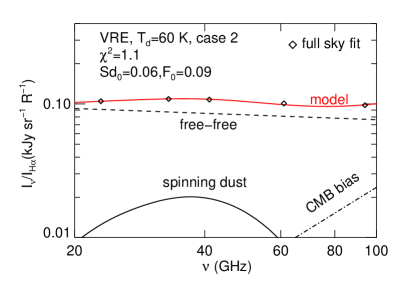
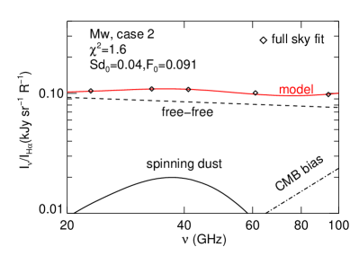
Figure 15.— A three-component fit model (solid line) to H${\alpha}$-correlated spectrum using CMB5 data (diamonds) from Dobler et al. (2009) for VRE (upper) and Mw (lower) regimes using case 2 ($\mu_{1}=0$) of ¯. Three components of free-free emission, spinning dust emission and CMB bias are shown separately. As shown are best fits parameters and $\chi^{2}$.

Dobler et al. (2009) have determined the spectrum $I^{\rm obs}$ of the H$\alpha$-correlated emission in the WMAP five-year data. The thermal dust contribution has been almost completely removed as part of the SFD- correlated component, and synchrotron emission has similarly been removed by its correlation with the Haslam et al. (1982) 408 MHz map. Within the frequency range considered here, the residual thermal dust emission and synchrotron emission are assumed negligible.

Thus, as in Dobler et al. (2009), we fit the H$\alpha$-correlated spectrum with three components: free-free emission, spinning dust emission, and CMB cross-correlation bias. We present the ratio of intensity to H$\alpha$ intensity. The free-free emission is given by (Draine 2011)

$$\frac{I_{\nu}^{\rm ff}}{I_{{\rm H}\alpha}}=F_{0}\left(\frac{\nu}{23\,{\rm GHz}}\right)^{-0.12}~{}{\rm kJy~{}sr}^{-1}{\rm R}^{-1}.$$ (61)

where

$$F_{0}=0.197T_{4}^{0.614+0.942\,{\rm ln}T_{4}}.$$ (62)

The CMB bias is defined as $\partial B_{\nu}(T)/\partial T|_{T=2.7~{}{\rm K}}\propto\nu^{2}$, and we obtain

$$\frac{I_{\nu}^{\rm cmb}}{I_{{\rm H}\alpha}}=C_{0}\left(\frac{\nu}{23\,{\rm GHz}}\right)^{2}\frac{1}{{\rm plc}(\nu)}~{}~{}{\rm kJy~{}sr}^{-1}{\rm R}^{-1},$$ (63)

where $C_{0}$ is a free parameter, and plc is the Planck correction factor to convert thermodynamic temperature $\Delta T$ to antenna temperature at frequency $\nu$.

The spinning dust component is taken as the emission from the WIM. We obtain

$$\frac{I_{\nu}^{{\rm sd}}}{I_{{\rm H}\alpha}} = Sd_{0}\times\left[\frac{I_{\nu}^{{\rm sd}}}{I_{{\rm H}\alpha}}\right]_{{\rm WIM}},~{}~{}~{}$$ (64)

where $\left[I_{\nu}^{{\rm sd}}/I_{{\rm H}\alpha}\right]_{{\rm WIM}}$ is calculated for our model for the WIM with a standard PAH abundance, and the fitting parameter $Sd_{0}$ allows for the possibility that the PAH abundance in the WIM may differ from our standard value.

Using Equation (60) for the above equation, we obtain the spinning dust intensity per H$\alpha$

$$\left[\frac{I_{\nu}^{{\rm sd}}}{I_{{\rm H}\alpha}}\right]_{{\rm WIM}} = \left(\frac{j_{\nu}}{n_{{\rm H}}}\right)_{{\rm WIM}}\times\left(\frac{n_{{\rm H}}}{j_{{\rm H}\alpha}}\right)_{{\rm WIM}},$$ (65)

$$= \left(\frac{j_{\nu}}{n_{{\rm H}}}\right)_{{\rm WIM}}\times\left(\frac{\,{\rm cm}^{-5}/n_{{\rm H}}}{(n_{e}/n_{{\rm H}})^{2}}\right)$$

$$\times\frac{8.55\times 10^{18}T_{4}^{0.942+0.031\,{\rm ln}T_{4}}}{\rm R}~{}{\rm kJy~{}sr}^{-1}.~{}~{}~{}~{}~{}~{}~{}~{}$$

The model emission intensity per H$\alpha$ is then

$$\frac{I_{\nu}^{\rm mod}}{I_{{\rm H}\alpha}} = \Biggl{\{}F_{0}\left(\frac{\nu}{23\,{\rm GHz}}\right)^{-0.12}+C_{0}\left(\frac{\nu}{23\,{\rm GHz}}\right)^{2}\frac{1}{{\rm plc}(\nu)}\Biggr{\}}~{}\frac{{\rm kJy~{}sr}^{-1}}{{\rm R}}$$ (66)

$$+Sd_{0}\times\left[\frac{I_{\nu}^{{\rm sd}}}{I_{{\rm H}\alpha}}\right]_{{\rm WIM}}.$$

For the spinning dust model, we consider a range of gas density $n_{{\rm H}}\in[0.01,1]\,{\rm cm}^{-3}$ and the value of dipole moment $\beta_{0}\in[0.1,1]$ D. For each ($n_{{\rm H}}$, $\beta_{0}$), we compute $\left(j_{\nu}/n_{{\rm H}}\right)_{{\rm WIM}}$. We then vary the values of $F_{0},Sd_{0}$ and $C_{0}$. From a given value $F_{0}$ we derive the gas temperature $T_{4}$ using Equation (62). When $T_{4}$ and $\left(j_{\nu}/n_{{\rm H}}\right)_{{\rm WIM}}$ are known, we obtain $\left[I_{\nu}^{{\rm sd}}/I_{{\rm H}\alpha}\right]_{{\rm WIM}}$ from Equation (65).

The fitting process is performed by minimizing the $\chi^{2}$ function

$$\chi^{2}=\sum_{\nu}\frac{|I^{\rm mod}_{\nu}-I^{\rm obs}_{\nu}|^{2}}{\sigma_{\nu}^{2}},$$ (67)

where $I_{\nu}^{\rm obs}$ is the measured H$\alpha$-correlated emission intensity, and $\sigma_{\nu}$ is the mean noise per observation at the frequency band $\nu$ (see Hinshaw et al. 2007; Dobler et al. 2009).

In general, $\chi^{2}$ is a function of three amplitude parameters $F_{0},C_{0},Sd_{0}$, and two physical parameters $n_{{\rm H}}$ and $\beta_{0}$. Therefore, the fitting proceeds by minimizing $\chi^{2}$ over five parameters.

Figure 14 shows $\chi^{2}$ contours as functions of $\beta_{0}$ and $n_{{\rm H}}$ for case 2 ($\mu_{1}=0$) and for VRE ($T_{{\rm d}}=60~{}{\rm K}$), for the values of $Sd_{0}$ and $F_{0}$ for which $\chi^{2}$ is minimized. We can see that the distribution of $\chi^{2}$ is localized and centered around the standard values in the plane $n_{{\rm H}}-\beta_{0}$.

Figure 15 shows the fit of the three-component model to the H$\alpha$-correlated foreground spectrum for VRE and Mw regimes for case 2 of ¯. Both regimes provide a good fit to the data.

Table 4 shows best fit parameters and $\chi^{2}$ for different cases of ¯ orientation and different regimes of internal relaxation. We can see that both orientations of ¯ (case 1 and case 2) can produce a good fit with low $\chi^{2}$, but case 2 exhibits a relatively better fit. The best fit gas density is in the range $0.08-0.15\,{\rm cm}^{-3}$. In case 1, the best fit dipole moment for the VRE and Mw regimes is $\beta_{0}\sim 0.76$ and $1.0$ D. In case 2, the best fit requires $\beta_{0}\sim 0.65$ D and $0.84$ D for VRE and Mw respectively. Case 1 requires higher $\beta_{0}$ to reproduce the observations than case 2 because the effect of grain shape irregularity is more important for case 1. Similarly, the Mw regime requires higher $\beta_{0}$ than VRE because the effect of irregularity is stronger for the former case.

From Table 4, it can be seen that the best fit value $Sd_{0}\sim 0.04-0.06$ is significantly lower than the value $Sd_{0}=0.3$ in Dobler et al. (2009). Our lower $Sd_{0}$ stems from the higher value of $\beta_{0}$ required, from the increase of emissivity in the HDL10 model compared to the DL98 model used in Dobler et al. (2009), and the further (modest) increase in emissivity for irregular grains. As a result, a higher depletion of small PAHs is required to obtain a good fit.

In addition, from best fit values $F_{0}$ in Table 4 we derive the gas temperature $T_{e}\sim 2700-3500$ K as found by Dobler et al. (2009). This is lower than the typical temperature $T_{e}=8000$ K usually assumed for the WIM. Dong & Draine (2011) proposed a model of three components that can explain the low gas temperature in the WIM.

Table 4 Best fit parameters and $\chi^{2}$ for H$\alpha$-correlated emission

¯	$f_{\rm int}(\theta)$	$n_{{\rm H}}~{}({\rm cm}^{-3})$	$\beta_{0}~{}({\rm D})$	$Sd_{0}$	$F_{0}$	$C_{0}$	$\chi^{2}$
case 1	VRE	0.15	0.76	0.04	0.09	0.0012	1.9
	Mw	0.08	1.0	0.06	0.1	0.001	4.5
case 2	VRE	0.11	0.65	0.06	0.09	0.0012	1.1
	Mw	0.14	0.84	0.04	0.09	0.0012	1.6

7.3. Fitting to thermal dust-correlated emission

In addition to the H$\alpha$-correlated emission, the foreground induces a dust-correlated emission spectrum with a usual thermal dust emission component falling from $94$ to $40$ GHz, and another component rising from $40$ to $23$ GHz (see Bennett et al. 2003). The latter component is consistent with the spinning dust emission (DL98ab; de Oliveira et al. 2004; HDL10). Although this peak frequency around $22$ GHz is consistent with prediction by the DL98 model, it is lower than the prediction by the improved model of HDL10, using the same parameters for the CNM as in DL98b.

As in Dobler et al. (2009), we fit the thermal dust-correlated emission spectrum with a three-component model including spinning dust, thermal dust and CMB bias.

Dobler et al. (1999) determined the spectrum $I_{\nu}/T_{94\,{\rm GHz}}({\rm FDS})$ for the contribution $I_{\nu}$ to the intensity from the thermal-dust-correlated emission, where $T_{94\,{\rm GHz}}({\rm FDS})$ is the antenna temperature at 94 GHz predicted for the FDS dust model (Finkbeiner, Davis & Schlegel 1999).

Planck collaboration (2011c) showed that the thermal dust emission can be approximated by

$${I_{\nu}^{\rm td}}=\epsilon(\nu)B_{\nu}(T_{\rm td})N_{{\rm H}},$$ (68)

where $T_{\rm td}=17.6~{}{\rm K}$ and $\epsilon({\nu})=0.92\times 10^{-25}(\lambda/250~{}\mu{\rm m})^{-1.8}\,{\rm cm}^{-2}{\rm H}^{-1}$.

We model the spinning dust contribution as

$${I_{\nu}^{{\rm sd}}}=Sd_{0}\left(\frac{j_{\nu}}{n_{{\rm H}}}\right)_{{\rm CNM}}.$$ (69)

Thus, we seek to fit the Dobler et al. (2009) spectrum by

$$\frac{I_{\nu}^{\rm mod}}{T_{94\,{\rm GHz}}({\rm FDS})} = \Biggl{\{}\left[\left(\frac{\nu}{94\,{\rm GHz}}\right)^{3.8}+Sd_{0}\frac{\left(j_{\nu}/n_{{\rm H}}\right)_{{\rm CNM}}}{[\epsilon(\nu)B_{\nu}(T_{\rm td})]_{\nu=94\,{\rm GHz}}}\right]$$ (70)

$$+C_{0}\left(\frac{\nu}{94\,{\rm GHz}}\right)^{2}\Biggr{\}}~{}{\rm kJy}\,{\rm sr}^{-1}{\rm m}{\rm K}^{-1},~{}$$

where $A,~{}Sd_{0}$ and $C_{0}$ are adjustable parameters. For each trial $n_{{\rm H}}$ and $\beta_{0}$, we adjust $A,~{}Sd_{0}$ and $C_{0}$ to minimize $\chi^{2}$. We consider different possible values of $n_{{\rm H}}$ and $\beta_{0}$.

Best fit parameters and $\chi^{2}$ for different situations are shown in Table 5. In case 1 ($\mu_{1}=\mu/\sqrt{3}$), the best fit corresponds to $n_{{\rm H}}=6.0-6.5\,{\rm cm}^{-3}$, and $\beta_{0}\sim 0.94-0.97~{}{\rm D}$ for VRE and Mw regimes. In case 2 ($\mu_{1}=0$), the best fit corresponds to $n_{{\rm H}}=7.0-7.5\,{\rm cm}^{-3}$ and $\beta_{0}\sim 0.95~{}{\rm D}$ for VRE and Mw regimes. The significance of fitting is low in both cases 1 and 2. Case 2 fits slightly better ($\chi^{2}=30-35$) than case 1 ($\chi^{2}=54-56$).

Figure 16 shows the best-fit to the thermal dust-correlated spectrum obtained using case 2 models, for both VRE and Mw regimes.

We see that the fitting to thermal dust-correlated emission has large $\chi^{2}$. The reason is that the curvature of the model spectrum is larger than that of the observed spectrum for frequencies $22-44$ GHz.

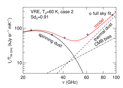
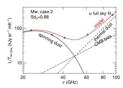
Figure 16.— A three-component fit model (solid line) to thermal dust-correlated emission spectrum (diamonds) for VRE ($T_{{\rm d}}=60~{}{\rm K}$, upper) and Mw (lower) regimes using case 2 ($\mu_{1}=0$) of ¯. Three components of spinning dust emission, thermal dust emission and CMB bias are shown separately but solid, dashed and dashed-dotted lines. As shown is the best fit value of $Sd_{0}$.

Table 5 Best fit parameters and $\chi^{2}$ for thermal dust-correlated emission

¯	$f_{\rm int}(\theta)$	$n_{{\rm H}}({\rm cm}^{-3})$	$\beta_{0}({\rm D})$	$Sd_{0}$	$A$	$C_{0}$	$\chi^{2}$
case 1	VRE	6.5	0.97	0.74	184.3	$4.5$	54
	Mw	6.0	0.94	0.63	176.1	$4.7$	56
case 2	VRE	7.5	0.95	0.91	192.4	$2.9$	30
	Mw	7.0	0.96	0.88	184.2	$3.5$	35

7.4. Classical vs. quantum treatment

Ysard & Verstraete (2010, hereafter YV10) questioned the validity of classical mechanics in the DL98 model for spinning dust emission. YV10 put forward a quantum-mechanical formalism for treating the rotational emission. However, they only calculated spinning dust emission for the rotational transition $\Delta J=-1$ and $\Delta K=0$, which is induced by the oscillation of the dipole component along the grain symmetry axis.

In our view, a quantum description of spinning dust is unnecessary, because, as shown in DL98b for spherical grain, the angular quantum number

$$J\equiv\frac{I_{1}\omega}{\hbar}\approx 72\left(\frac{N_{\rm C}}{20}\right)^{5/6}\left(\frac{T_{\rm rot}}{100~{}{\rm K}}\right)^{1/2},$$ (71)

which shows that even smallest PAHs have angular quantum number $J\gg 1$, therefore, the classical treatment should be valid.

Miville-Deschênes et al. (2008) made an attempt to separate the spinning dust component from the Galactic foreground components (mostly synchrotron and anomalous emission) using both the WMAP intensity and polarization data. The inferred spinning dust spectrum is presented in Figure 17 (diamond symbols).

Ysard, Miville-Deschênes & Verstraete (2010) presented a fit to observation data for spinning dust, which is extracted from WMAP data for regions with latitude $b=22.4^{\circ}$ (the spinning dust spectrum extracted from WMAP data using the quantum mechanical approach from YV10). They assumed a lower cut-off of the grain size corresponding to the number of carbon atom $N_{\min}=24$ and $48$ for the CNM and WNM, and dipole moment $\beta_{0}=0.3~{}{\rm D}$. Converting to the grain size using the usual relationship $a=10(N_{{\rm C}}/410)^{1/3}\,{\rm\AA}$, we obtain $a_{\min}\sim 3.88$ and $4.89\,{\rm\AA}$, respectively. However, since $a_{\min}$ chosen for the WNM is much larger than that for the CNM, the peak frequency of its emission spectrum is expected to be much lower than that for the CNM, because the peak frequency decreases with $a_{\min}$ increasing (see §5.2). This disagrees with results shown in Figure 5 of Ysard et al. (2010), where the peak frequency of the WNM ($\nu_{{\rm peak}}\sim 45$ GHz) is much larger than that for the CNM ($\nu_{{\rm peak}}\sim 22$ GHz).

To see how well the improved model of spinning dust in HDL10 fits to observation data for selected regions in Ysard et al. (2010), we assume the same spinning dust parameters as in Ysard et al. (i.e. gas density, dipole moment $\beta_{0}$ and $a_{\min}$).

The total emission intensity from the CNM and WNM with column density $N_{{\rm H}}$(CNM) and $N_{{\rm H}}$(WNM) is given by

$$I_{\nu}^{\rm mod}=N_{{\rm H}}({\rm CNM})\left(\frac{j_{\nu}^{{\rm sd}}}{n_{{\rm H}}}\right)_{\rm CNM}+N_{{\rm H}}({\rm WNM})\left(\frac{j_{\nu}^{{\rm sd}}}{n_{{\rm H}}}\right)_{\rm WNM},~{}~{}~{}$$

where $\left[{j_{\nu}^{{\rm sd}}}/{n_{{\rm H}}}\right]$ is the spinning dust emissivity per H calculated for the CNM and WNM, respectively (see Table 2). The fitting proceeds by minimizing $\chi^{2}$ (Eq. 67) with $N_{{\rm H}}$(CNM) and $N_{{\rm H}}$(WNM) as free parameters. We found that the best fit is achieved at $N_{{\rm H}}({\rm CNM})=3.5\times 10^{20}\,{\rm cm}^{-2}$ and $N_{{\rm H}}({\rm WNM})=1.4\times 10^{21}\,{\rm cm}^{-2}$. The best fit is shown in Figure 17 and $\chi^{2}$ is also shown. We can see that our improved model can reproduce the observational data for high latitude regions.

Figure 17.— Comparison of our study with the anomalous spectrum extracted from the observation data in YV10. The solid line is the total emissivity resulting from the CNM and WNM with $N_{{\rm H}}({\rm CNM})=3.5\times 10^{20}\,{\rm cm}^{-2}$ and $N_{{\rm H}}({\rm WNM})=1.4\times 10^{21}\,{\rm cm}^{-2}$. Squared symbols show observation data. All grains have the characteristic electric dipole moment $\beta=\beta_{0}=0.3~{}{\rm D}$. Case 2 ($\mu_{1}=0$) of ¯ is considered.

8. Discussion

8.1. Relative importance of effects

The present paper extends further the improved model of spinning dust emission in HDL10 by including the following effects: irregular grain shape, dust temperature fluctuations due to transient heating, orientation of dipole moment, and fluctuations of gas density due to compressible turbulence.

8.1.1 Power Spectrum of Grains of Irregular Shape

First of all, we find that a torque-free rotating irregular grain radiates at multiple frequency modes with angular frequency $\omega_{m_{i}}$ and $\omega_{n_{i}}$ depending on a dimensionless parameter $q$, the ratio of the rotational energy to the rotational energy along the axis of major inertia.

In case 1 ($\mu_{1}=\mu/\sqrt{3}$) of ¯ orientation, the mode $\omega_{m_{-1}}$ dominates the dipole emission for $q$ close to $1$ (when ${\bf a}_{1}$ makes a small angle with ${\bf J}$). As $q$ increases, the mode $\omega_{m_{0}}$ increases accordingly, and become dominant. Physically, the mode $\omega_{m=0}$ arises from the precession of the dipole moment component parallel to ${\bf a}_{1}$ axis about the angular momentum. Its emission power increases with the angle $\theta$ between ${\bf a}_{1}$ and ${\bf J}$, and is maximum when ${\bf a}_{1}$ is perpendicular to ${\bf J}$, i.e., $\theta=\pi/2$ or $q=q_{{\rm sp}}$.

In case 2 ($\mu_{1}=0$, i.e. no dipole component along ${\bf a}_{1}$), the mode $m=0$ does not exist when the grain rotates about ${\bf a}_{1}$ for $q<q_{{\rm sp}}$. For $q>q_{{\rm sp}}$, the irregular grain rotates about ${\bf a}_{3}$, therefore, the dipole moment component along ${\bf a}_{3}$ induces the frequency mode $m=0$.

In both case 1 and case 2, the modes $m=\pm 1$, which result from the oscillation of dipole moments along ${\bf a}_{2}$ and ${\bf a}_{3}$, always exist, and have power increasing with $q$ up to $q=q_{{\rm sp}}$, then decrease in importance as $q$ increases further.

8.1.2 Increase of spinning dust emission with the degree of grain shape irregularity

For both case 1 ($\mu_{1}=\mu/\sqrt{3}$) and 2 ($\mu_{1}=0$) of ¯ orientation, we find that the peak frequency increases rapidly with increasing degree of grain shape irregularity $\eta$ (see §4.3). The underlying reason is that the deformation of the grain from the disk-like shape allows the grain to rotate along the axis of minimum moment of inertia ${\bf a}_{3}$, in addition to rotation about ${\bf a}_{1}$ and ${\bf a}_{2}$ axes. For a given angular momentum, the angular velocity along ${\bf a}_{3}$ is largest, so that the emission frequency of the irregular grain is in general higher than that of the disk-like grain with the same mass.

Peak emissivity also increases with the grain shape irregularity for case 1. But for case 2, $j_{{\rm peak}}$ decreases with $\eta$ for $T_{{\rm vib}}\leq 60~{}{\rm K}$, and starts to increase with $\eta$ as $T_{{\rm vib}}$ increases.

When the internal thermal fluctuations are rather weak ($T_{J}>T_{{\rm vib}}$) so that the grain tends to rotate with the minimum rotational energy, $\theta$ and $q$ deviate slightly from $\theta=0$ and $q=1$, and the rotational emission spectrum of irregular grains differs only slightly from that of disk-like grains. In contrast, for strong thermal fluctuations ($T_{J}\ll T_{{\rm vib}}$), the thermal fluctuations enable grains to spend an important fraction of time rotating with large $q$. Because the total power emission increases with $q$, the higher probability of rotating with larger $q$ results in larger emissivity and peak frequency than disk-like grains.

8.1.3 Orientation of dipole moment

We investigated the effects of changing the orientation of the electric dipole moment ¯. We found (see Fig. 9) that as the orientation is varied from having a component parallel to ${\bf a}_{1}$ (case 1, $\mu_{1}=\mu/\sqrt{3}$) to being entirely perpendicular to ${\bf a}_{1}$ (case 2, $\mu_{1}=0$), the peak frequency $\nu_{{\rm peak}}$ and the peak emissivity both decrease by $\sim 10\%$. Given the sensitivity of the spectrum to other variables (mass distribution, $|\mu|$, grain shape, gas density, gas temperature), it does not seem possible to infer the orientation of ¯ from observations of the spectrum.

8.1.4 Density Fluctuation due to Compressible Turbulence

We identified interstellar turbulence as another factor that influences emission spectrum. The spinning dust emissivity is determined by two principal processes: collisional and radiative damping and excitation. Local compression due to turbulence increases the collisional excitation, that results in increased spinning dust emissivity. We found that the emission is increased by a factor from $1.2-1.4$ as the sonic Mach number increases from $M_{\,{\rm s}}=2-7$.

8.2. Constraints from Spinning dust Emission

Recent studies showed that the correspondence of the DL98 model to observations can be improved by adjusting the parameters of the model. For instance, the five-year (WMAP) data showed a broad bump with frequency at $\sim 40$ GHz in the H$\alpha$-correlated emission (Dobler & Finkbeiner 2008; Dobler et al. 2009). Using H$\alpha$ as a tracer of the WIM, they showed that this bump can be explained using the DL98 model by varying either dipole moment or gas density of the WIM.

By fitting the 3 components of synchrotron, free-free emission and spinning dust emission to H$\alpha$-correlated spectrum, Dobler et al. (2009) found that the spinning dust model with $\beta_{0}=0.15$ D and density $n_{{\rm H}}=0.15\,{\rm cm}^{-3}$ could reproduce the observed spectrum, with $\nu_{{\rm peak}}=37\,{\rm GHz}$. Our best fit values from the improved model correspond to $n_{{\rm H}}=0.08-0.15\,{\rm cm}^{-3}$ and $\beta_{0}$ in the range of $0.6-1.0$ D.

In addition to the H$\alpha$-correlated emission, WMAP data show a thermal dust- correlated spectrum that declines from $23$ GHz to $40$ GHz. This peak at low frequency is lower than the HDL10 model prediction using the standard parameters for the CNM.

Our results show that the thermal dust-correlated data can be fitted with spinning dust emission from the CNM of density $n_{{\rm H}}\sim 6-8\,{\rm cm}^{-3}$ and $\beta_{0}\sim 0.95-1.0~{}{\rm D}$. Similar to Dobler et al. (2009), we also found that the best-fit model did not provide a very good fit (high $\chi^{2}$). The reason for that is the rotational spectrum is steeper than the observation data in frequency range $20-50$ GHz. Dobler et al. (2009) suggested that the superposition of spinning dust spectra from different ISM phases along a sight-line would produce a flatter spectral slope. With our results for irregular grains, one can see that by averaging the rotational spectrum over various degree of irregularity $\eta$ with the fraction of irregular grains decreasing with $\eta$ (see §4), the obtained spectrum becomes shallower, that can improve the fit.

8.3. Range of applicability of the model of spinning dust emission

The model of spinning dust emission has been used to interpret the anomalous microwave emission in the general ISM (e.g. Finkbeiner 2004; Dobler & Finkbeiner 2008; Gold et al. 2009, 2011; Planck Collaboration 2011c), in star forming regions in the nearby galaxy NGC 6946 (Scaife et al. 2010; Murphy et al. 2010) and in the Persus and Ophiuchus clouds (Cassasus et al. 2008; Tibbs et al. 2010; Planck Collaboration 2011a). Early Planck results have been interpreted as showing an emission excess from spinning dust in the Magellanic Clouds (Bot et al. 2010; Planck Collaboration 2011b).

This paper together with HDL10 presents a comprehensive model of spinning dust, accounting for non-disk-like (“irregular”) grains, new electric dipole emission modes from torque-free rotation of irregular grains, and investigating the effects of variation in grain dipole moment, gas density, and different regimes of vibrational-rotational mode coupling. We believe that apart from being an important CMB foreground, the spinning dust spectrum can become an important diagnostic tool to constrain physical properties of astrophysical dust (e.g. size distribution, shape, electric dipole moment and gas density) in various environments.

9. Summary

The model of spinning dust emission is further extended by accounting for effects of irregular grain shape, fluctuations of dust temperature, and effects of ISM turbulence. We consider both regimes of fast internal relaxation and without internal relaxation. Our main results are as follows.

1. Small grains of irregular shape radiate in general at multiple harmonic frequency modes. The rotational emission shifts to higher frequency as the degree of grain shape irregularity increases, but the spectral profile remains similar. The effect of the grain shape irregularity is more important for higher dust temperature or stronger internal thermal fluctuations. Depending on the irregularity parameter $\eta$, peak frequency and peak emissivity can be increased by a factor of up to $1.4$, relative to disk-likes grains of the same mass (see Figs. 5 and 6) for case 1 ($\mu_{1}=\mu/\sqrt{3}$).

2. Fluctuations of dust temperature $T_{{\rm vib}}$ also increase the rotational emissivity relative to the emissivity for grains of a steady low temperature.

3. Fluctuations of gas density and gas pressure due to compressible turbulence enhance both emission and peak frequency of spinning dust spectrum compared to that in uniform media. An increase in emission by a factor from $1.2-1.4$ is expected as the sonic Mach number $M_{\,{\rm s}}$ increases from $2-7$.

4. Spinning dust parameters (e.g., gas density and dipole moment) are constrained by fitting the improved model to WMAP cross-correlation foreground spectra, including H$\alpha$ and thermal dust-correlated spectra. We find a reduced PAH abundance in the WIM ($Sd_{0}\approx 0.05$) with dipole moment parameter $\beta_{0}\approx 0.7$ D. For the thermal-dust-correlated emission, we find a normal PAH abundance ($Sd_{0}\approx 0.9$) and $\beta_{0}\approx 0.95$ D.

5. Our improved model also provides a good fit to WMAP data for selected regions at high latitude ($b=22.4^{\circ}$) obtained by Ysard et al. (2010).

Appendix A A. Electric Dipole emission from an irregular grain

A.1. A1. Torque-free motion

The effective size $a$ of an irregular grain with volume $V$ is defined as the radius of a sphere with the same volume $V$, i.e.,

$$a=\left(3V/4\pi\right)^{1/3}.$$ (A1)

In general, an irregular grain can be characterized by a triaxial ellipsoid with moments of inertia $I_{1},I_{2}$ and $I_{3}$ around three principal axes ${\bf a}_{1},{\bf a}_{2}$ and ${\bf a}_{3}$, respectively. Define dimensionless parameters $\alpha_{i}$ so that the moments of inertia are written as

$$I_{j}=\alpha_{j}I_{\rm sph},$$ (A2)

where $I_{\rm sph}=\left(8\pi/15\right)\rho a^{5}$ is the moment of inertia of the equivalent sphere of radius $a$, and $\rho$ is the mass density of the grain.

For a torque-free rotating grain, its angular momentum ${\bf J}$ is conserved , while the angular velocity ! nutates and wobbles with respect to ${\bf J}$. We can term the wobbling associated with the irregularity in the grain shape irregular wobbling, to avoid confusion with thermal wobbling (also thermal fluctuations) induced by the Barnett relaxation (Purcell 1979) and nuclear relaxation (Lazarian & Draine 1999b).

A detailed description of the torque-free motion for an asymmetric top in terms of Euler angles $\theta,\phi$ and $\psi$ (see Fig. 1) can be found in classical textbooks (e.g. Landau & Lifshitz 1976; see also WD03), and a brief summary is given below.

Consider an ellipsoid with three principal axes ${\bf a}_{1},{\bf a}_{2},{\bf a}_{3}$ and moments of inertia $I_{1}>I_{2}>I_{3}$.

Let define a dimensionless quantity

$$k^{2}=\frac{(I_{2}-I_{3})(q-1)}{(I_{1}-I_{2})(1-I_{3}q/I_{1})},$$ (A3)

where $q={2I_{1}E_{\rm rot}}/{J^{2}}$ is the ratio of total kinetic energy to the rotational energy along the axis of major inertia ${\bf a}_{1}$.

(a) For $q<I_{1}/I_{2},k^{2}<1$, the solution of Euler equations is

$$\omega_{1} =\pm\frac{J}{I_{1}}\left(\frac{I_{1}-I_{3}q}{I_{1}-I_{3}}\right)^{1/2}\mbox{dn}(\tau),$$ (A4)

$$\omega_{2} =-\frac{J}{I_{2}}\left(\frac{I_{2}(q-1)}{I_{1}-I_{2}}\right)^{1/2}\mbox{sn}(\tau),$$ (A5)

$$\omega_{3} =\pm\frac{J}{I_{3}}\left(\frac{I_{3}(q-1)}{I_{1}-I_{3}}\right)^{1/2}\mbox{cn}(\tau)$$ (A6)

where cn, sn and dn are hyperbolic trigonometric functions, and $\tau$ is given by

$$\tau\equiv tJ\left[\frac{(I_{1}-I_{2})(1-I_{3}q/I_{1})}{I_{1}I_{2}I_{3}}\right]^{1/2},$$ (A7)

and the sign $\pm$ in $\omega_{1}$ and $\omega_{3}$ are taken the same. We denote the rotation with $+$ and $-$ sign as positive and negative rotation state. For $q<I_{1}/I_{2}$, the grain mostly rotate about the axis of major inertia ${\bf a}_{1}$, while it rotates about ${\bf a}_{3}$ for $q>I_{1}/I_{2}$.

The rotation period around the axis of major inertia ${\bf a}_{1}$ is

$$P_{\tau}=4F(\pi/2,k^{2}),$$ (A8)

where $F$ is the elliptic integral defined by

$$F(\epsilon,m)=\int_{0}^{\epsilon}d\theta(1-m\sin^{2}\theta)^{-1/2}.$$ (A9)

(b) For $q>I_{1}/I_{2}$, angular velocities are given by

$$\omega_{1} =\pm\frac{J}{I_{1}}\left(\frac{I_{1}-I_{3}q}{I_{1}-I_{3}}\right)^{1/2}\mbox{cn}(\tau),$$ (A10)

$$\omega_{2} =-\frac{J}{I_{2}}\left(\frac{I_{2}(1-I_{3}q)}{I_{2}-I_{3}}\right)^{1/2}\mbox{sn}(\tau),$$ (A11)

$$\omega_{3} =\pm\frac{J}{I_{3}}\left(\frac{I_{3}(q-1)}{I_{1}-I_{3}}\right)^{1/2}\mbox{dn}(\tau),$$ (A12)

where

$$\tau\equiv tJ\left[\frac{(I_{2}-I_{3})(q-1)}{I_{1}I_{2}I_{3}}\right]^{1/2}.$$ (A13)

Rotation period for this case is given by

$$P_{\tau}=4F(\pi/2,k^{-2}).$$ (A14)

(c) For $q\sim I_{1}/I_{3}$, Equation (A3) shows that $k^{2}\rightarrow\infty$, the rotation of the grain is about the axis near ${\bf a}_{3}$. Thus, $\omega_{3}\approx J/I_{3}$, and $\omega_{1}\sim\omega_{2}\sim 0$. From Euler equations, we obtain

$$\frac{I_{1}{\rm d}\omega_{1}}{dt}=\omega_{2}\omega_{3}\left(I_{2}-I_{3}\right),$$ (A15)

$$\frac{I_{2}{\rm d}\omega_{2}}{dt}=\omega_{3}\omega_{1}\left(I_{3}-I_{1}\right).$$ (A16)

Substituting $\omega_{3}=\Omega_{0}=J/I_{3}$, the equations are rewritten as

$$\frac{dJ_{1}}{dt}=\Omega_{0}J_{2}\left(1-\frac{I_{3}}{I_{2}}\right),$$ (A17)

$$\frac{dJ_{2}}{dt}=-\Omega_{0}J_{1}\left(1-\frac{I_{3}}{I_{1}}\right),$$ (A18)

where $J_{k}=I_{k}\omega_{k}$. Taking the first derivative of Equation (A17), and using (A18), we obtain solutions for $J_{1}$ and $J_{2}$:

$$J_{1} = A\cos\omega t,$$ (A19)

$$J_{2} = \frac{A}{\omega}\left(1-\frac{I_{3}}{I_{1}}\right)\sin\omega t=\frac{A}{\left(1-{I_{3}}/{I_{2}}\right)^{1/2}}\left(1-\frac{I_{3}}{I_{1}}\right)^{1/2}\sin\omega t,$$ (A20)

where $\omega^{2}=\Omega_{0}^{2}\left(1-\frac{I_{3}}{I_{2}}\right)\left(1-\frac{I_{3}}{I_{1}}\right)$, and $A$ is a constant of integration. Denote $A/\left(1-\frac{I_{3}}{I_{2}}\right)^{1/2}=\alpha J$ with $\alpha$ is a small parameter, then

$$J_{1}=\alpha J\left(1-\frac{I_{3}}{I_{2}}\right)^{1/2}\cos\omega t,$$ (A21)

$$J_{2}=\alpha J\left(1-\frac{I_{3}}{I_{1}}\right)^{1/2}\sin\omega t.$$ (A22)

The value of $\alpha$ is found by using the relation

$$q=\frac{2I_{1}E}{J^{2}},$$ (A23)

$$E=\frac{J_{1}^{2}}{2I_{1}}+\frac{J_{3}^{2}}{2I_{3}},$$ (A24)

where we have use the fact that at $t=0$, $J_{2}=0$. Substituting $J_{1}$ and $J_{3}$ in Equation (A24) and plugging it into (A23), we obtain

$$q=\alpha^{2}\left(\frac{I_{3}}{I_{2}}-1\right)+\frac{I_{1}}{I_{3}},$$ (A25)

Hence,

$$\alpha=\left(\frac{I_{1}/I_{3}-q}{1-I_{3}/I_{2}}\right)^{1/2}$$ (A26)

As $q=I_{1}/I_{3}$, then $\alpha=0$, i.e., $J_{1}=J_{2}=0$ and $J_{3}=J$.

When the angular velocity components are known, we can infer the orientation of the grain axes in the inertial coordinate system using Euler angles:

$$\cos\theta=\frac{I_{1}\omega_{1}}{J},~{}~{}~{}\tan\psi=\frac{I_{2}\omega_{2}}{I_{3}\omega_{3}}.$$ (A27)

A.2. A2. Flip states

For a given ${\bf J}$, there are two sets of solution ($\pm$ sign) for $\omega_{i}$ of the Euler motion equations (see Eqs A4-A6). It can be seen that for $q<q_{{\rm sp}}$, two rotation states $\pm$ correspond to $\omega_{1}>0$ and $\omega_{1}<0$, i.e., ${\bf a}_{1}.{\bf J}>0$ and ${\bf a}_{1}.{\bf J}<0$. We define these rotation states as positive flip state and negative flip state (also WD03; Hoang & Lazarian 2008). For $q>q_{{\rm sp}}$, the similar situation occurs with $\omega_{3}$, and there are positive and negative flip states with respect to ${\bf a}_{3}$.

A.3. A3. Electric Dipole Emission for Irregular Grain

Let us consider the general case where the dipole is fixed in the grain body, and given by

$${\hbox{\boldsym\char 22\relax}}=\mu_{1}{\bf a}_{1}+\mu_{2}{\bf a}_{2}+\mu_{3}{\bf a}_{3}.$$ (A28)

where $\mu_{i}$ are components of electric dipoles along three principal axes. In Paper I we disregarded the third term in Equation (A28) because of grain’s axisymmetry.

In the inertial coordinate system $\hat{\bf x}\hat{\bf y}\hat{\bf z}$ (see Fig. 1), ${\bf a}_{1},{\bf a}_{2}$ and ${\bf a}_{3}$ are described as

$${\bf a}_{1} = \sin\phi\sin\theta\hat{\bf x}-\cos\phi\sin\theta\hat{\bf y}+\cos\theta\hat{\bf z},$$ (A29)

$${\bf a}_{2} = (\cos\phi\cos\psi-\sin\phi\sin\psi\cos\theta)\hat{\bf x}+(\sin\phi\cos\psi+\cos\phi\sin\psi\cos\theta)\hat{\bf y}+\sin\psi\sin\theta\hat{\bf z},$$ (A30)

$${\bf a}_{3} = -(\cos\phi\sin\psi+\sin\phi\cos\psi\cos\theta)\hat{\bf x}+(-\sin\phi\sin\psi+\cos\phi\cos\psi\cos\theta)\hat{\bf y}+\cos\psi\sin\theta\hat{\bf z},~{}$$ (A31)

where $\phi,\psi$ and $\theta$ are Euler angles.

Complex motion of the grain principal axes with respect to ${\bf J}$ results in an acceleration for dipole moment in the inertial coordinate system $\hat{\bf x}\hat{\bf y}\hat{\bf z}$:

$$\ddot{{\hbox{\boldsym\char 22\relax}}}=\mu_{1}\ddot{{\bf a}}_{1}+\mu_{2}\ddot{{\bf a}}_{2}+\mu_{3}\ddot{{\bf a}_{3}},$$ (A32)

where $\ddot{{\bf a}}_{1}$ and $\ddot{{\bf a}}_{2}$ are given by

$$\ddot{{\bf a}}_{1} = \left[-(\dot{\phi}^{2}+\dot{\theta}^{2})\sin\phi\sin\theta+\dot{\theta}\dot{\phi}\cos\phi\cos\theta\right]\hat{\bf x}$$ (A33)

$$+\left[\dot{\phi}^{2}\sin\theta\cos\phi+\dot{\theta}^{2}\cos\phi\sin\theta+\dot{\theta}\dot{\phi}\sin\phi\cos\theta\right]\hat{\bf y}-\dot{\theta}^{2}\cos\theta\hat{\bf z},$$

$$\ddot{{\bf a}}_{2} = \left[-(\dot{\phi}^{2}+\dot{\psi}^{2})(\cos\phi\cos\psi-\sin\phi\sin\psi\cos\theta)-2\dot{\phi}\dot{\psi}(-\sin\phi\sin\psi+\cos\phi\cos\psi\cos\theta)\right]\hat{\bf x}$$ (A34)

$$+\left[\dot{\theta}^{2}\sin\phi\sin\psi\cos\theta+\dot{\theta}\dot{\phi}\cos\phi\sin\psi\sin\theta+\dot{\theta}\dot{\psi}\sin\phi\cos\psi\sin\theta\right]\hat{\bf x}$$

$$+\left[-(\dot{\phi}^{2}+\dot{\psi}^{2})(\sin\phi\cos\psi+\cos\phi\sin\psi\cos\theta)-2\dot{\phi}\dot{\psi}(\cos\phi\sin\psi+\sin\phi\cos\psi\cos\theta)\right]\hat{\bf y}$$

$$+\left[-\dot{\theta}^{2}\cos\phi\sin\psi\cos\theta+\dot{\theta}\dot{\phi}\sin\phi\sin\psi\sin\theta-\dot{\theta}\dot{\psi}\cos\phi\cos\psi\sin\theta\right]\hat{\bf y}$$

$$+\left[-({\dot{\psi}}^{2}+\dot{\theta}^{2})\sin\psi\sin\theta+\dot{\theta}\dot{\psi}\cos\psi\cos\theta\right]\hat{\bf z},$$

$$\ddot{{\bf a}}_{3} = \left[(\dot{\phi}^{2}+\dot{\psi}^{2})(\cos\phi\sin\psi+\sin\phi\cos\psi\cos\theta)+2\dot{\phi}\dot{\psi}(\sin\phi\cos\psi+\cos\phi\sin\psi\cos\theta)\right]\hat{\bf x}$$ (A35)

$$+\left[\dot{\theta}^{2}\sin\phi\cos\psi\cos\theta+\dot{\theta}\dot{\phi}\cos\phi\cos\psi\sin\theta-\dot{\theta}\dot{\psi}\sin\phi\sin\psi\sin\theta\right]\hat{\bf x}$$

$$+\left[(\dot{\phi}^{2}+\dot{\psi}^{2})(\sin\phi\sin\psi-\cos\phi\cos\psi\cos\theta)-2\dot{\phi}\dot{\psi}(\cos\phi\cos\psi-\sin\phi\sin\psi\cos\theta)\right]\hat{\bf y}$$

$$+\left[-\dot{\theta}^{2}\cos\phi\cos\psi\cos\theta+\dot{\theta}\dot{\phi}\sin\phi\cos\psi\sin\theta+\dot{\theta}\dot{\psi}\cos\phi\sin\psi\sin\theta\right]\hat{\bf y}$$

$$+\left[-({\dot{\psi}}^{2}+\dot{\theta}^{2})\cos\psi\sin\theta-\dot{\theta}\dot{\psi}\sin\psi\cos\theta\right]\hat{\bf z},$$

The precession and rotation rates $\dot{\phi}$ and $\dot{\psi}$ are related to the angular velocity components as follows (Landau & Lifshitz 1976):

$$\omega_{1}=\dot{\phi}\cos\theta+\dot{\psi},$$ (A36)

$$\omega_{2}=\dot{\phi}\sin\theta\sin\psi+\dot{\theta}\cos\psi,$$ (A37)

$$\omega_{3}=\dot{\phi}\sin\theta\cos\psi-\dot{\theta}\sin\psi.$$ (A38)

By solving equations, we obtain

$$\dot{\theta}=\omega_{2}\cos\psi-\omega_{3}\sin\psi,$$ (A39)

$$\dot{\phi}=\frac{\omega_{2}\sin\psi+\omega_{3}\cos\psi}{\sin\theta}={J}\frac{I_{2}\omega_{2}^{2}+I_{3}\omega_{3}^{2}}{I_{2}^{2}\omega_{2}^{2}+I_{3}^{2}\omega_{3}^{2}},$$ (A40)

$$\dot{\psi}=\omega_{1}-\dot{\phi}\cos\theta,~{}~{}$$ (A41)

Plugging into Equation (A32) with the usage of Equations (A33) and (A34) we obtain the acceleration components as functions of time. Performing Fourier transform for these components gives us the spectrum of electric dipole emission (see Fig. 2).

The dipole emission power of this torque-free rotating grain can be obtained by averaging the $\ddot{\mu}^{2}$ over time:

$$P_{{\rm ed}}=\frac{2}{3c^{3}}\langle\ddot{\hbox{\boldsym\char 22\relax}}^{2}\rangle\equiv\frac{1}{T}\int_{0}^{T}\frac{2}{3c^{3}}\ddot{\hbox{\boldsym\char 22\relax}}^{2}dt$$ (A42)

Appendix B B. Electric dipole damping for disk-like grain

In the grain body system ${\bf a}_{1}{\bf a}_{2}{\bf a}_{3}$, the dipole moment is given by Equation (A28). The orientation of axes ${\bf a}_{i}$ in an inertial system are determined by Euler angles (see Fig. 1). The increase of grain’s angular momentum over time arising from the acceleration of dipole emission is then

$$\frac{d{{\bf J}}}{dt}=-\frac{2}{3c^{3}}[\dot{{\hbox{\boldsym\char 22\relax}}}\times\ddot{{\hbox{\boldsym\char 22\relax}}}],$$ (B1)

Using Equations (A28) and (A32) for (B1) and averaging it over $\phi$ and $\psi$ from 0 to $2\pi$ due to torque-free motion, the non- vanished component is given by

$$\frac{d{J_{z}}}{dt}=-\frac{2}{3c^{3}}\frac{J^{3}}{I_{\|}^{3}}\left[\frac{\mu_{\perp}^{2}}{2}\{\cos^{4}\theta(h^{3}-3h+2)+\cos^{2}\theta(3h-2h^{3})+h^{3}\}+\mu_{1}^{2}h^{3}\sin^{2}\theta\right],$$ (B2)

where we assumed $\mu_{2}^{2}=\mu_{3}^{3}=\mu_{\perp}^{2}/2$. The components $dJ_{x}/dt$ and $dJ_{y}/dt$ are averaged out to zero.

For case 1 with $\mu_{\|}:\mu_{\perp}=2:3$, i.e., $\mu_{1}^{2}=\mu_{2}^{2}=\mu_{3}^{2}=\mu^{2}/3$, we obtain (similar to HDL10):

$$\frac{dJ_{z}}{dt}=-\frac{2\mu^{2}}{9c^{3}}\frac{J^{3}}{I_{\|}^{3}}\left[\cos^{4}\theta(h^{3}-3h+2)+\cos^{2}\theta(-2h^{3}+3h)+h^{3}(1+\sin^{2}\theta)\right]$$ (B3)

For case 2 with $\mu_{\|}:\mu_{\perp}=0:1$, i.e., $\mu_{1}=0$ and $\mu_{2}^{2}=\mu_{3}^{2}=\mu^{2}/2$,

$$\frac{dJ_{z}}{dt}=-\frac{\mu^{2}}{3c^{3}}\frac{J^{3}}{I_{\|}^{3}}\left[\cos^{4}\theta(h^{3}-3h+2)+\cos^{2}\theta(-2h^{3}+3h)+h^{3}\right].$$ (B4)

In dimensionless variables, we have

$$\frac{dJ_{z}^{\prime}}{dt^{\prime}}=-\frac{2}{3}\frac{J_{z}^{{}^{\prime}3}}{\tau^{\prime}_{{\rm ed},{\rm eff}}},$$ (B5)

where $\tau^{\prime}_{{\rm ed},{\rm eff}}=\tau_{{\rm ed},{\rm eff}}/\tau_{{\rm H},\|}$ with

$$\tau_{{\rm ed},{\rm eff}} = \tau_{{\rm ed},\|}\times\frac{2}{\cos^{4}\theta(h^{3}-3h+2)+\cos^{2}\theta(-2h^{3}+3h)+h^{3}(1+\sin^{2}\theta)},$$ (B6)

$$\tau_{{\rm ed},\|} = \frac{3I_{\|}^{2}c^{3}}{4k_{\rm B}T_{\,{\rm gas}}\mu^{2}},$$ (B7)

for case 1, and

$$\tau_{{\rm ed},{\rm eff}} = \tau_{{\rm ed},\|}\times\frac{2}{\cos^{2}\theta(-2h^{3}+3h)+\cos^{4}\theta(h^{3}-3h+2)+h^{3}},$$ (B8)

$$\tau_{{\rm ed},\|} = \frac{I_{\|}^{2}c^{3}}{2k_{\rm B}T_{\,{\rm gas}}\mu^{2}},$$ (B9)

for case 2.

For $\theta=0$, then $\tau_{{\rm ed},{\rm eff}}=\tau_{{\rm ed},\|}$.

References

- (1) Ali-Haïmoud, Y., Hirata, C. M., & Dickinson, C. 2009, MNRAS, 395, 1055
- (2) Armstrong, J. W., Rickett, B. J., & Spangler, S. R. 1995, ApJ, 443, 209
- (3) Bennett, C. L. et al. 2003, ApJS, 148, 97
- (4) Bouchet, F. R., Prunet, S.,& Sethi, Shiv K. 1999, MNRAS, 302, 663
- (5) Burkhart, B., Falceta-Gonçalves, D., Kowal, G., & Lazarian, A. 2009, ApJ, 693, 250
- (6) Burkhart, B., Stanimirović, S., Lazarian, A., & Kowal, G. 2010, ApJ, 708, 120
- (7) Chepurnov, A., & Lazarian, A. 2010, ApJ, 710, 853
- (8) de Oliveira-Costa et al. 1999, ApJ, 527, 9
- (9) de Oliveira-Costa et al. 2002, ApJS, 567, 363
- (10) de Oliveira-Costa et al. 2004, ApJ, 606, L89
- (11) Dobler, G., Finkbeiner, D. 2008, ApJ, 680, 1222
- (12) Dobler, G., Draine, B. T., & Finkbeiner, D. P. 2009, ApJ, 699, 1374
- (13) Dong, R., & Draine, B. T. 2011, ApJ, 727, 35
- (14) Draine, B. T., & Anderson, N. 1985, ApJ, 292, 494
- (15) Draine, B. T., & Lazarian, A. 1998, ApJ, 494, L19 (DL98a)
- (16) Draine, B. T., & Lazarian, A. 1998, ApJ, 508, 157 (DL98b)
- (17) Draine, B. T., & Li, A. 2001, ApJ, 551, 807
- (18) —. 2007, ApJ, 657, 810 (DL07)
- (19) Draine, B. T. 2011, Physics of the Interstellar and Intergalactic Medium (Princeton, NJ: Princeton Univ. Press)
- (20) Efstathiou, G. 2003, MNRAS, 346,26
- (21) Erickson, W. C, 1957, ApJ, 126, 480
- (22) Esquivel A and Lazarian A 2010, ApJ, 710, 125
- (23) Ferrara, A., & Dettmar, R.-J. 1994, ApJ, 427, 155
- (24) Finkbeiner, D. P., Davis, M., & Schlegel, D. J. 1999, ApJ, 524, 867 (FDS)
- (25) Finkbeiner, D. P., Langston, G. I., & Minter, A. H. 2004, ApJ, 617, 350
- (26) Gold, B., Bennett, C. L., Hill, R. S., et al. 2009, ApJS, 180, 265
- (27) Gold, B., Odegard, N., Weiland, J. L., et al. 2011, ApJS, 192, 15
- (28) Greenberg,J. M. 1968, in Stars and Stellar Systems, Vol. 7, ed. B. M. Middlehurst & L. H. Aller (Chicago: Univ. Chicago Press), 221)
- (29) Haslam, C. G. T., Stoffel, H., Salter, C. J., & Wilson, W. E. 1982, A&AS, 47, 1
- (30) Harris, F. J. 1978, Proc. IEEE, 66, 51
- (31) Hoang, T., & Lazarian, A. 2008, MNRAS, 388, 117
- (32) Hoang, T., & Lazarian, A. 2009, ApJ, 695, 1457
- (33) Hoang, T., Draine, B. T., & Lazarian, A. 2010, ApJ, 715, 1462 (HDL10)
- (34) Jones, R.V., & Spitzer, L. 1967, ApJ, 147, 943
- (35) Kowal, G., Lazarian, A., & Beresnyak, A. 2007, ApJ, 658, 423
- (36) Kogut, A. et al. 1996a, ApJ, 460,1
- (37) Kogut, A. et al. 1996a, ApJ, 464, 5
- (38) Landau, L. D., & Lifshitz. E. M. 1976, Mechanics (Oxford: Perganon)
- (39) Lazarian, A. 2007, J. Quant. Spectrosc. Rad. Trans., 106, 225
- (40) Lazarian, A., & Draine, B.T. 1999, ApJ, 520, L67
- (41) Lazarian A., & Efroimsky M. 1999, MNRAS, 303, 673
- (42) Lazarian, A., & Finkbeiner, D. 2003, New Astronomy Revies, 47, 1107
- (43) Lazarian, A., & Hoang, T. 2009, arXiv 0901.0146
- (44) Lazarian, A., & Roberge, W. 1997, ApJ, 484, 230
- (45) Li, A., & Draine, B. T. 2001, ApJ, 554, 778
- (46) Mathis, J.S., Mezger, P. G., & Panagia, N. 1983, A&A, 128, 212
- (47) Murphy, E. J., et al. 2010, ApJ, 709L, 108
- (48) Purcell, E. M. 1979, ApJ, 231, 404.
- (49) Planck Collaboration. 2011a, Planck early results: New light on Anomalous Emission from Spinning Dust Grains (Submitted to A&A), arXiv 1101.2031
- (50) Planck Collaboration. 2011b, Planck early results: Origin of the submillimetre excess dust emission in the Magellanic Clouds (Submitted to A&A), arXiv 1101.2046
- (51) Planck Collaboration. 2011c, Planck Early Results: Properties of the interstellar medium in the Galactic plane (Submitted to A&A), arXiv 1101.2032
- (52) Rafikov, R. R. 2006, ApJ, 646, 288
- (53) Roberge, W., DeGraff, T. A., & Flaherty, J. E. 1993, ApJ, 418, 287
- (54) Scaife, A. M., Nikolic B., Green D. et al. 2010, MNRAS, 406, L45
- (55) Silsbee, K., Ali-Haïmoud, Y., & Hirata, C. 2011, MNRAS, 411, 2750
- (56) Sironi, L., & Draine, B. T. 2009, ApJ, 698, 1292
- (57) Tegmark, M., et al. 2000, ApJ, 530, 133
- (58) Tibbs, C. T., et al. 2010, MNRAS, 402, 1969
- (59) Townes, C., & Schawlow, A. 1955, Microwave Spectroscopy (New York: McGraw-Hill)
- (60) Ysard, N., & Verstraete, L. 2010, A&A, 509, A12 (YV10)
- (61) Ysard, N., Miville-Deschenes, M. A., & Verstraete, L. 2010, A&A, 509, L1
- (62) Weingartner, J. C., & Draine, B. T. 2003, ApJ, 589, 289