Quantitative reliability of Migdal-Eliashberg theory for strong electron-phonon coupling

Abstract

We reassess the validity of Migdal-Eliashberg (ME) theory for coupled electron-phonon systems for large couplings $\lambda$. Although model calculations have found that ME theory breaks down for $\lambda\sim 0.5$, it is routinely applied for $\lambda>1$ to strong coupling superconductors. To resolve this discrepancy it is important to distinguish between bare parameters, used as input in models, and effective parameters, derived from experiments. We show explicitly that ME gives accurate results for the critical temperature and the spectral gap for large effective $\lambda$. This provides quantitative theoretical support for the applicability of ME theory to strong coupling conventional superconductors.

I Introduction

The theory of conventional superconductivity, where pairing is mediated by the coupling of electrons to lattice vibrations, is considered as one of the major achievements of the twentieth century condensed matter physics. It is based on the relatively simple Eliashberg equations,Eliashberg (1960) where vertex corrections are neglected. The application of these equations is justified by Migdal’s theorem,Migdal (1958) which states that vertex corrections are proportional to the effective coupling strength $\lambda$ and the ratio of phonon $\omega_{\rm ph}$ and electronic energy scale $W$, which usually is of the order $1/100$ and less.Carbotte (1990); Marsiglio and Carbotte (2008) The properties of the superconducting state in Migdal-Eliashberg (ME) theory are then largely determined by $\lambda$, $\omega_{\rm ph}$ and a phenomenological parameter for the Coulomb repulsion $\mu^{*}$. ME theory is also routinely used as a standard pairing theory for other situations where a bosonic pairing mechanism is analyzed.Chubukov et al. (2008); Dahm et al. (2009)

A number of studies mainly based on the Holstein model, which go beyond the ME theory, have illustrated that vertex corrections cannot be neglected for large coupling strength even if the ratio $\omega_{\rm ph}/W$ is very small and that the ME theory becomes inaccurate whendif $\lambda$ exceeds a certain value.Benedetti and Zeyher (1998); Alexandrov (2001); Meyer et al. (2002); Capone and Ciuchi (2003); Hague and d’Abrumenil (2008) In the adiabatic limit, Benedetti and Zeyher Benedetti and Zeyher (1998) found a breakdown of Migdal’s theorem due to the appearance of additional extremal paths in the action for $\lambda\gtrsim 0.4$.dif Capone and Ciuchi Capone and Ciuchi (2003) found quantitative deviations of self-consistent ME calculations from DMFT already for intermediate coupling strengths and qualitatively different behavior for stronger coupling. Alexandrov Alexandrov (2001) argued that even in the adiabatic limit ME theory breaks down due to bipolaron formation and symmetry breaking when $\lambda$ exceeds one. For strong coupling superconductors values of $\lambda$ of the order 1-3 are commonly quoted.Carbotte (1990); Marsiglio and Carbotte (2008) The model calculations therefore suggest that strong coupling superconductors do not lie within the range of applicability of the ME theory.

The purpose of this paper is to bring the results from the model studies in a form that they can be compared in a meaningful way to the standard diagrammatic approach for superconductivity. This allows us to clarify the quantitative reliability of ME theory for relevant values of $\lambda$ and $\omega_{\rm ph}/W$. If phonon renormalization occurs it is necessary to distinguish the bare model parameters from the effective parameters describing the phonon properties.Maksimov and Khomskii (1982); Marsiglio (1990); Dolgov et al. (2008) The latter correspond to the ones derived from experiment or density functional calculations. We study the Holstein model in the limit where the lattice has infinite dimensions. In this limit the dynamical mean field theory (DMFT) Georges et al. (1996) becomes exact. These DMFT results serve as a benchmark for ME calculations.

We show in qualitative agreement with earlier work in the normal phase Capone and Ciuchi (2003) that self-consistent ME calculations become inaccurate already at moderate bare coupling both for electronic and phonon properties. However in contrast with previous interpretations, we show that at these bare couplings the effective coupling is very large, larger than for strong coupling superconductors. For effective couplings relevant for strong coupling superconductors the ME theory is still accurate.

In many applications of ME theory the phonons are not calculated self-consistently, but taken as an input either from a different calculation or experiment. Then one is interested in how accurately electronic properties are described by the ME equations for a given phonon spectrum. We can check this explicitely by taking DMFT as a benchmark for electronic properties and providing the full phonon spectrum as an input for the ME calculations (termed ME+ph later). We show that the electronic properties are predicted very reliably up to large effective coupling strengths within ME+ph calculations, i.e. with an accuracy of better than 10%. In this paper we will neglect the effect of the Coulomb interaction usually taken into account via the parameter $\mu^{*}$.

The paper is structured as follows: In Sec. II, we first recall the usual definition of the pairing function $\alpha^{2}F(\omega)$ and the coupling strength $\lambda$. Then we give explicit details for the DMFT and ME approaches. In Sec. III, results for the comparison of the DMFT and ME calculations are shown, followed by the conclusions in Sec. IV.

II Model and formalism

II.1 Pairing function

The pairing function $\alpha^{2}F(\omega)$ is an essential ingredient for conventional superconductivity. It can be defined by Carbotte (1990); Marsiglio and Carbotte (2008)

$$\alpha_{{\bm{k}},{\bm{k}}^{\prime}}^{2}F(\omega)=\rho_{0}|g_{{\bm{k}},{\bm{k}}^{\prime}}|^{2}\rho^{D}_{{\bm{k}}-{\bm{k}}^{\prime}}(\omega),$$ (1)

where $\rho_{0}$ is the electronic density of states at the Fermi level, $g_{{\bm{k}},{\bm{k}}^{\prime}}$ the electron-phonon coupling matrix element and $\rho^{D}_{{\bm{q}}}(\omega)$ the phonon spectral function, related to the phonon propagator as

$$D_{{\bm{q}}}(i\omega_{m})=\!\int\limits_{0}^{\infty}\!\!{\rm d}\omega\;\rho^{D}_{{\bm{q}}}(\omega)\frac{2\omega}{(i\omega_{m})^{2}-\omega^{2}}.$$ (2)

These are the dressed phonon quantities of the interacting system. In conventional theory these are often taken from experiment or estimated by a different method, and then inserted in the Eliashberg equations to solve for $T_{c}$, the spectral gap and other properties. As the properties of conventional superconductivity are mostly confined to a small window around the Fermi energy, often a Fermi surface average is used,

$$\alpha^{2}F(\omega)=\frac{1}{\rho_{0}^{2}}\sum_{{\bm{k}},{\bm{k}}^{\prime}}\alpha_{{\bm{k}},{\bm{k}}^{\prime}}^{2}F(\omega)\delta(\varepsilon_{{\bm{k}}}-\mu)\delta(\varepsilon_{{\bm{k}}^{\prime}}-\mu).$$ (3)

Then the superconducting state is largely determined through the coupling constantMcMillan (1968); Allen and Dynes (1975); Marsiglio and Carbotte (2008) $\lambda$,

$$\lambda=2\!\int\limits_{0}^{\infty}\!\!{\rm d}\omega\;\frac{\alpha^{2}F(\omega)}{\omega}.$$ (4)

II.2 Holstein model and DMFT approach

Our quantitative test of the ME theory is based on a model, which has been frequently used in the literature, the Holstein model,

$$H = -\sum_{i,j,{\sigma}}(t_{ij}c^{\dagger}_{i,\sigma}c_{j,\sigma}+\mathrm{h.c.})+\omega_{0}\sum_{i}b_{i}^{\dagger}b_{i}$$

$$+g\sum_{i}(b_{i}+b_{i}^{\dagger})\Big{(}\sum_{\sigma}\hat{n}_{i,\sigma}-1\Big{)}.$$

$c^{\dagger}_{i,\sigma}$ creates an electron at lattice site $i$ with spin $\sigma$, and $b_{i}^{\dagger}$ a phonon with oscillator frequency $\omega_{0}$, $\hat{n}_{i,\sigma}=c^{\dagger}_{i,\sigma}c_{i,\sigma}$. The electronic density is coupled to an optical phonon mode with coupling constant $g$. We have set the ionic mass to $M=1$ in (II.2). The local oscillator displacement is related to the bosonic operators by $\hat{x}_{i}=(b_{i}+b_{i}^{\dagger})/\sqrt{2\omega_{0}}$, where $\hbar=1$.

For the DMFT at $T=0$ we solve the effective impurity problem with the numerical renormalization group Wilson (1975); Bulla et al. (2008) (NRG) adapted to the case with symmetry breaking.Bauer and Hewson (2009); Bauer et al. (2009) For the logarithmic discretization parameter is $\Lambda=1.8$, and we keep about 1000 states at each iteration. The initial bosonic Hilbert space is restricted to a maximum of 50 states. We use a semi-elliptic density of states (DOS) for the electrons $\rho_{0}(\varepsilon)=\sqrt{4t^{2}-\varepsilon^{2}}/(2\pi t^{2})$ with bandwidth $W=4t$. In terms of the Hilbert transform ${\rm HT}[\rho_{0}](z)$ we have for the diagonal Green’s function

$$G_{11}(i\omega_{n})=A_{G}{\rm HT}[\rho_{0}](\varepsilon_{+})+B_{G}{\rm HT}[\rho_{0}](\varepsilon_{-}),$$ (6)

and for the off-diagonal part

$$G_{21}(i\omega_{n})=A_{F}{\rm HT}[\rho_{0}](\varepsilon_{+})+B_{F}{\rm HT}[\rho_{0}](\varepsilon_{-}).$$ (7)

We have defined $A_{G}=(\zeta_{2}(i\omega_{n})+\varepsilon_{+}(i\omega_{n}))/(\varepsilon_{+}(i\omega_{n})-\varepsilon_{-}(i\omega_{n}))$, $B_{G}=(\zeta_{2}(i\omega_{n})+\varepsilon_{-}(i\omega_{n}))/(\varepsilon_{-}(i\omega_{n})-\varepsilon_{+}(i\omega_{n}))$ $A_{F}=\Sigma_{21}(i\omega_{n})/(\varepsilon_{+}(i\omega_{n})-\varepsilon_{-}(i\omega_{n}))$, and $B_{F}=\Sigma_{21}(i\omega_{n})/(\varepsilon_{-}(i\omega_{n})-\varepsilon_{+}(i\omega_{n}))$, where

$$\varepsilon_{\pm} = \frac{\zeta_{1}(i\omega_{n})-\zeta_{2}(i\omega_{n})}{2}\pm$$

$$\frac{1}{2}\sqrt{(\zeta_{1}(i\omega_{n})+\zeta_{2}(i\omega_{n}))^{2}-4\Sigma_{21}(i\omega_{n})\Sigma_{12}(i\omega_{n})},$$

with $\zeta_{1}(z)=z+\mu-\Sigma_{11}(z)$ and $\zeta_{2}(z)=z-\mu-\Sigma_{22}(z)$. For the Nambu Green’s functions we have $G_{12}(i\omega_{n})=G_{21}(i\omega_{n})$ and $G_{22}(i\omega_{n})=-G_{11}(-i\omega_{n})$. This implies $\Sigma_{12}(i\omega_{n})=\Sigma_{21}(i\omega_{n})$ and $\Sigma_{22}(i\omega_{n})=-\Sigma_{11}(-i\omega_{n})$ for the self-energies. At half filling $G_{11}(i\omega_{n})$ and $\Sigma_{11}(i\omega_{n})$ are imaginary functions, whereas $G_{21}(i\omega_{n})$ and $\Sigma_{21}(i\omega_{n})$ and $D(i\omega_{m})$ and $\Sigma_{{\rm ph}}(i\omega_{m})$ are real functions. For the semi-elliptic DOS the Hilbert transform is given by

$${\rm HT}[\rho_{0}](z)=\!\int\limits_{-D}^{D}\!\!{\rm d}\varepsilon\;\frac{\rho_{0}(\varepsilon)}{z-\varepsilon}=\frac{1}{2t^{2}}\Big{(}z-{\rm sgn}(\mathrm{Im}(z))\sqrt{z^{2}-4t^{2}}\Big{)},$$ (9)

where the square root of a complex number $w$ is given by $\sqrt{r}\mathrm{e}^{i\varphi/2}$, where $\varphi=[0,2\pi)$, such that the imaginary part of $\sqrt{w}$ is positive.

At finite temperature, we use the continuous-time quantum Monte Carlo (QMC) method developed for electron-phonon systems.Assaad and Lang (2007) To calculate $T_{c}$ we study the susceptibility in the pairing channel $\chi({\bm{q}},i\omega_{n})$ in the limit ${\bm{q}}\to 0$ and $i\omega_{n}\to 0$. It can be expressed in terms of the irreducible vertex in the particle-particle channel $\Gamma^{(\rm pp)}$, which is calculated in the QMC procedure.Georges et al. (1996) It is then sufficient to analyze when the largest eigenvalue of the symmetric matrix,

$$M_{n_{1},n_{2}}=\frac{1}{\beta}\sqrt{\tilde{\chi}^{0}(i\omega_{n_{1}})}[\Gamma^{(\rm pp)}(i\omega_{n_{1}},i\omega_{n_{2}};0)]\sqrt{\tilde{\chi}^{0}(i\omega_{n_{2}})},$$ (10)

exceeds one. We have defined the pair propagator,Georges et al. (1996)

$$\tilde{\chi}^{0}(i\omega_{n_{1}})=\frac{G(i\omega_{n_{1}})-G(-i\omega_{n_{1}})}{\zeta(-i\omega_{n_{1}})-\zeta(i\omega_{n_{1}})},$$ (11)

$\zeta(i\omega_{n})=i\omega_{n}+\mu-\Sigma(i\omega_{n})$, where $G(i\omega_{n_{1}})$ is the local lattice Green’s function in the normal state.

II.3 ME approach

Figure 1: Diagrams for diagonal and offdiagonal self-energy in ME theory involving the full electronic Green’s function $G$ and anomalous part $F$ and the full phonon propagator $D$.

The matrix equation for the electronic self-energies in ME theory (see Fig. 1) reads

$$\underline{\Sigma}(i\omega_{n})=-\frac{1}{\beta}\sum_{m}g^{2}\tau_{3}\underline{G}(i\omega_{m}+i\omega_{n})\tau_{3}D(i\omega_{m}),$$ (12)

where

$$\underline{G}_{{\bm{k}}}(i\omega_{n})^{-1}=\underline{G}^{0}_{{\bm{k}}}(i\omega_{n})^{-1}-\underline{\Sigma}(i\omega_{n})$$ (13)

with $G_{ij}(i\omega_{n})=\sum_{{\bm{k}}}G_{ij,{\bm{k}}}(i\omega_{n})$ and $\underline{G}^{0}_{{\bm{k}}}(i\omega_{n})^{-1}=i\omega_{n}-\tau_{3}(\varepsilon_{{\bm{k}}}-\mu)$. Notice that we use the form valid for large coordination number, such that only local lattice Green’s functions enter. These are calculated with the same semi-elliptic DOS as in Eqs. (6) and (7) for the DMFT calculation. Thus by ME theory we mean the diagrammatic theory, which neglects all vertex corrections to (12), and this is compared to the full DMFT results. No further approximation such as assuming a constant density of states or large bandwidth are made. The latter are common approximations in the literature on ME theory,Carbotte (1990); Marsiglio and Carbotte (2008) whose accuracy can be analyzed in an expansion in $\omega_{\rm ph}/W$. This is, however, not the subject of the present paper, where we focus entirely on the accuracy of the theory when vertex corrections are neglected.

The pairing function reads $\alpha^{2}F(\omega)=\rho_{0}g^{2}\rho^{D}(\omega)$ for the Holstein model. In the non-interacting limit we have $\rho^{D}_{0}(\omega)=\delta(\omega-\omega_{0})-\delta(\omega+\omega_{0})$, which in Eq. (4) gives $\lambda_{0}=\rho_{0}2g^{2}/\omega_{0}$ purely in terms of bare parameters. This quantity was used in model studies and denoted by $\lambda$.dif However, $\lambda$ as defined in Eq. (4) is given for the interacting system.Maksimov and Khomskii (1982); Marsiglio (1990); Dolgov et al. (2008) Then the phonons are renormalized via the self-energy $\Sigma_{{\rm ph}}(i\omega_{m})$,

$$D(i\omega_{m})^{-1}=D^{0}(i\omega_{m})^{-1}-\Sigma_{{\rm ph}}(i\omega_{m}),$$ (14)

where $D^{0}(i\omega_{m})=2\omega_{0}/[(i\omega_{m})^{2}-\omega_{0}^{2}]$. The lowest order contribution to the phonon self-energy is

$$\Sigma_{{\rm ph}}(i\omega_{m})=\frac{2g^{2}}{\beta}\sum_{n}G(i\omega_{n})G(i\omega_{m}+i\omega_{n}).$$ (15)

As in Ref. Capone and Ciuchi, 2003 we will call Eqs. (15) and (12) self-consistent ME approximation. In the superconducting state an additional contribution from the off-diagonal Green’s function could be taken into account, which is however small and it will be neglected in the following.

We define the peak of the interacting phonon spectral function $\rho^{D}(\omega)$ as the effective phonon scale $\omega_{\rm ph}=\omega_{0}^{r}$. There is then a mapping of the bare dimensionless parameters $\lambda_{0},\omega_{0}/t$ to the effective parameters $\lambda,\omega_{0}^{r}/t$. $\lambda$ exceeds the bare $\lambda_{0}$ due to the phonon renormalization, $\omega_{0}\to\omega_{0}^{r}$, and due to the increased lattice fluctuations as shown in the identity valid at $T=0$,

$$w_{D}=\!\int\limits_{0}^{\infty}\!\!{\rm d}\omega\;\rho^{D}(\omega)=2\omega_{0}\langle\hat{x}^{2}\ \!\!\rangle,$$ (16)

which is generally larger than one. For a sharply peaked phonon spectrum the first moment sum rule,

$$\!\int\limits_{-\infty}^{\infty}\!\!{\rm d}\omega\;\omega\rho_{D}(\omega)=2\omega_{0},$$ (17)

implies $w_{D}\simeq\omega_{0}/\omega_{0}^{r}$. From an estimate for the phonon softening due to the lowest order diagram, $\omega^{r}_{0}/\omega_{0}=\sqrt{1-a\lambda_{0}}$, and Eq. (4) one can then obtain the result $\lambda=\lambda_{0}/(1-a\lambda_{0})$.Migdal (1958); Maksimov and Khomskii (1982); Dolgov et al. (2008) In three dimensions $a=2$, and for a semi-elliptic DOS in the limit of large dimensions we have $a=8/3$.

In order to calculate the gap at $T=0$ we solve equation (12) both by introducing spectral functions and analytic continuation to the real axis and for comparison directly on the imaginary axis. $D(i\omega_{m})$ can be calculated self-consistently via Eq. (15) or taken as an input from DMFT calculations. The latter type of calculation is termed ME+ph. In the ME theory $T_{c}$ is calculated by first finding the local lattice Green’s function $G(i\omega_{n})$ in the normal phase using

$$\Sigma(i\omega_{n})=-\frac{g^{2}}{\beta}\sum_{m}G(i\omega_{m}+i\omega_{n})D(i\omega_{m}),$$ (18)

and then employing Eq. (10) with

$$\Gamma^{(\rm pp)}(i\omega_{n_{1}},i\omega_{n_{2}};0)=-g^{2}D(i\omega_{n_{1}}-i\omega_{n_{2}}).$$ (19)

III Results

Let us first of all establish how the bare and effective quantities are related at $T=0$. At half filling for fixed $\omega_{0}=0.1t$, we plot $\lambda$ in Fig. 2 (a) and $\omega_{0}^{r}/\omega_{0}$ in Fig. 2 (b) both as function of $\lambda_{0}$. We show the results from self-consistent ME theory on the real axis (RA) and on the imaginary axis (IA) in comparison with the full DMFT-NRG result.

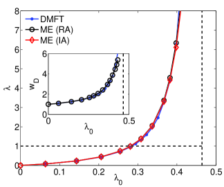
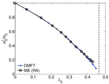
Figure 2: (Color online) Comparison of the selfconsistent ME and DMFT results for renormalized quantities as a function of the bare $\lambda_{0}$: (a) The effective coupling $\lambda$ as defined by Eq. (4), inset $w_{D}$ as given by Eq. (16). (b) The ratio of renormalized and bare phonon frequency $\omega_{0}^{r}/\omega_{0}$.

$\lambda$ increases slowly for $\lambda_{0}\leq 0.3$ up to values around one. Then it rises more rapidly close to values of $\lambda_{0}$ where in the normal state a metal to bipolaronic (BP) insulator transition had been found at $\lambda_{0}^{c}\simeq 0.464$ (shown as a vertical line).Benedetti and Zeyher (1998); Meyer et al. (2002) The behavior is qualitatively similar to the analytic estimate above, however, as $\lambda_{0}^{c}$>$1/a$ the latter is a substantial overestimate and diverges too quickly. The region of most interest for our purpose is $\lambda\sim 1-3$, typical values for strong coupling superconductors. This corresponds to $\lambda_{0}\sim 0.3-0.37$ in terms of bare parameters. The values for $\lambda$ obtained in the self-consistent ME theory compare well to the DMFT results for smaller values of $\lambda_{0}\leq 0.3$, and then start to overestimate this quantity slightly. For values of $\lambda_{0}$ closer to the BP transition self-consistent ME underestimates $\lambda$. We also compare the effective phonon frequency which decreases with $\lambda_{0}$ towards zero when $\lambda_{0}$ approaches $\lambda_{0}^{c}$. This quantity compares well to the DMFT result for a considerable range of $\lambda_{0}$, but starts to deviate for $\lambda_{0}>0.38$ or $\lambda\gtrsim 4$.

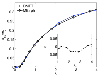
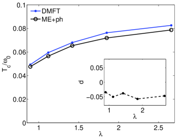
Figure 3: (Color online) Comparison of quantities for the superconducting state as a function of $\lambda$ obtained from DMFT and ME calculations with phonon input from DMFT (ME+ph): (a) The spectral gap $\Delta_{\rm sp}$; the inset shows the relative deviation $d$. (b) The critical temperature for the onset of superconductivity $T_{c}$.

We can also calculate electronic properties like the quasiparticle weight $z$ or the offdiagonal self-energy $\Sigma^{\rm off}(0)$ which roughly determines the spectral gap at zero temperature, $\Delta_{\rm sp}\simeq z\Sigma^{\rm off}(0)$. Then one finds good agreement for small coupling and moderate deviations between DMFT and self-consistent ME theory in the intermediate coupling regime, and close to the bipolaronic transition, similar to the results for $z$ and $\omega_{0}^{r}$ which have been obtained by Ciuchi and Capone Capone and Ciuchi (2003) in the normal state.

Our main objective is to test the validity of the ME theory at strong coupling. Hence, we compare the results for the superconducting properties $\Delta_{\rm sp}$ and $T_{c}$ obtained from the ME+ph calculations with the full DMFT results. In Fig. 3 (a) we show $\Delta_{\rm sp}$ as extracted from the spectral function computed from ME+ph calculations on the real axis and the corresponding DMFT result. Notice that the results are plotted as a function of $\lambda$ now.

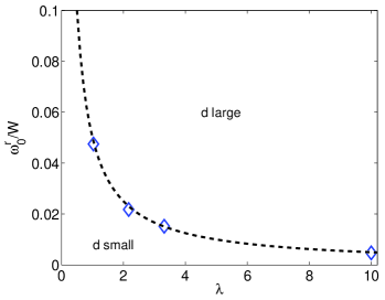
Figure 4: (Color online) Guideline for the quantitative reliability of ME theory. The diagram shows points (diamonds) in the $\omega_{0}^{r}/W$-$\lambda$-plane where the deviation $d$ between the DMFT and ME+ph theory is $d\simeq 0.1$. The dashed line is given by the functional form $\omega_{0}^{r}/W=c/\lambda$, which follows from an analytical estimate where vertex correction exceed a certain value. $c=0.05$ was used.

We find very good agreement for small values of $\lambda<1$, then a regime where ME+ph slightly underestimates the value for the gap, before it exceeds the DMFT result for larger values of $\lambda$. By inspecting the relative deviation $d=(\Delta_{\rm sp}^{\rm ME}-\Delta_{\rm sp}^{\rm DMFT})/\Delta_{\rm sp}^{\rm ME}$ plotted as an inset we see that there is an agreement in the regime $\lambda\sim 1-3$ better than 10%. At very large values of $\lambda$, $\Delta_{\rm sp}$ from ME+ph increases stronger than the DMFT result. For similar parameters we have also calculated the critical temperature $T_{c}$ as deduced from the Bethe-Salpeter equation of the uniform pair susceptibility.Han et al. (2003) The comparison of ME theory and DMFT-QMC result is shown in Fig. 3 (b). Good agreement is found in the relevant range for $\lambda$. DMFT-QMC systematically slightly underestimates the phonon renormalization, which accounts partly for the discrepancy of $T_{c}$ from the ME+ph calculations. In a related approach Marsiglio found for a 4$\times$4 cluster that the self-consistent ME theory agrees well with QMC calculations for the pairing susceptibility.Marsiglio (1990)

By doing similar comparisons for different bare parameters we mapped out for which values of the effective parameters $\lambda$ and $\omega_{0}^{r}/W$ DMFT and ME+ph show good agreement, i.e. $d\lesssim 0.1$. The results are shown in Fig. 4 and can be well understood in terms of the effective expansion parameter of ME theory $\lambda\omega_{0}^{r}/W$, which should not exceed 0.05 for good accuracy. The results can serve as a guideline for the application of ME theory with reliable phonon input.

IV Conclusions

We have assessed the validity of the ME theory. We calculated accurately the effective coupling strength $\lambda$ in terms of the bare coupling strength $\lambda_{0}$. For intermediate $\lambda_{0}$ the system is close to a bipolaronic metal-insulator transition and $\lambda$ is very strongly enhanced. Close to this point ME theory breaks down. However, for typical values for strong coupling superconductors, $\lambda\sim 1-3$, the ME theory is very accurate for small values of $\omega_{\rm ph}/W$. This result is demonstrated explicitly for the Holstein model in the limit of large dimensions, where most of the spectral weight of the pairing function is located at $\omega_{\rm ph}$. We expect that this result is also applicable for more general forms of pairing functions $\alpha^{2}F(\omega)$ in three dimensions with an appropriate cut-off scale $\omega_{\rm ph}$. In many applications of ME theory a momentum average over the Fermi surface is taken, such that the situation is similar to the one studied here. However, the momentum dependence can be important in certain cases especially for lower dimensional materials. For instance in Ref. Grimaldi et al., 1995, the momentum dependence of vertex corrections and their effect on $T_{c}$ was analyzed.

Acknowledgments

We wish to thank F. F. Assaad, A.C. Hewson, G. Sangiovanni, and R. Zeyher for helpful discussions, and to M. Kulic for pointing out Ref. Maksimov and Khomskii, 1982 to us. JH acknowledges support from the grant NSF DMR-0907150.

References

- Eliashberg (1960) G. M. Eliashberg, Sov. Phys. JETP 11, 696 (1960).
- Migdal (1958) A. B. Migdal, Sov. Phys. JETP 7, 996 (1958).
- Carbotte (1990) J. P. Carbotte, Rev. Mod. Phys. 62, 1027 (1990).
- Marsiglio and Carbotte (2008) F. Marsiglio and J. Carbotte, in Superconductivity (Vol 1), edited by K. Bennemann and J. Ketterson (Springer, Berlin, 2008).
- Chubukov et al. (2008) A. Chubukov, D. Pines, and J. Schmalian, in Superconductivity (Vol 2), edited by K. Bennemann and J. Ketterson (Springer, Berlin, 2008).
- Dahm et al. (2009) T. Dahm, V. Hinkov, S. V. Borisenko, A. A. Kordyuk, V. B. Zabolotnyy, J. Fink, B. Büchner, D. J. Scalapino, W. Hanke, and B. Keimer, Nature Phys. 5, 217 (2009).
- (7) The definition of can vary from ours by numerical prefactors, for instance in Ref. Benedetti and Zeyher, 1998 or in Ref. Capone and Ciuchi, 2003. The definition in Ref. Alexandrov, 2001 corresponds to ours. As emphasized in this paper bare and renormalized quantities have to be distinguished.
- Benedetti and Zeyher (1998) P. Benedetti and R. Zeyher, Phys. Rev. B 58, 14320 (1998).
- Alexandrov (2001) A. S. Alexandrov, Europhys. Lett. 56, 92 (2001).
- Meyer et al. (2002) D. Meyer, A. C. Hewson, and R. Bulla, Phys. Rev. Lett. 89, 196401 (2002).
- Capone and Ciuchi (2003) M. Capone and S. Ciuchi, Phys. Rev. Lett. 91, 186405 (2003).
- Hague and d’Abrumenil (2008) J. Hague and N. d’Abrumenil, J. Low Temp. Phys. 151, 1149 (2008).
- Maksimov and Khomskii (1982) E. Maksimov and D. Khomskii, in High temperature Superconductivity, edited by V. Ginzburg and D. Kirzhnits (Consultants Publisher, New York, 1982).
- Marsiglio (1990) F. Marsiglio, Phys. Rev. B 42, 2416 (1990).
- Dolgov et al. (2008) O. V. Dolgov, O. K. Andersen, and I. I. Mazin, Phys. Rev. B 77, 014517 (2008).
- Georges et al. (1996) A. Georges, G. Kotliar, W. Krauth, and M. Rozenberg, Rev. Mod. Phys. 68, 13 (1996).
- McMillan (1968) W. L. McMillan, Phys. Rev. 167, 331 (1968).
- Allen and Dynes (1975) P. B. Allen and R. C. Dynes, Phys. Rev. B 12, 905 (1975).
- Wilson (1975) K. Wilson, Rev. Mod. Phys. 47, 773 (1975).
- Bulla et al. (2008) R. Bulla, T. Costi, and T. Pruschke, Rev. Mod. Phys. 80, 395 (2008).
- Bauer and Hewson (2009) J. Bauer and A. C. Hewson, Europhys. Lett. 85, 27001 (2009).
- Bauer et al. (2009) J. Bauer, A. C. Hewson, and N. Dupuis, Phys. Rev. B 79, 214518 (2009).
- Assaad and Lang (2007) F. F. Assaad and T. C. Lang, Phys. Rev. B 76, 035116 (2007).
- Han et al. (2003) J. E. Han, O. Gunnarsson, and V. H. Crespi, Phys. Rev. Lett. 90, 167006 (2003).
- Grimaldi et al. (1995) C. Grimaldi, L. Pietronero, and S. Strässler, Phys. Rev. Lett. 75, 1158 (1995).