New metric tensors for anisotropic mesh generation

Abstract.   A new anisotropic mesh adaptation strategy for finite element solution of elliptic differential equations is presented. It generates anisotropic adaptive meshes as quasi-uniform ones in some metric space, with the metric tensor being computed based on a posteriori error estimates proposed in [36]. The new metric tensor explores more comprehensive information of anisotropy for the true solution than those existing ones. Numerical results show that this approach can be successfully applied to deal with poisson and steady convection-dominated problems. The superior accuracy and efficiency of the new metric tensor to others is illustrated on various numerical examples of complex two-dimensional simulations.

Keywords. anisotropic; mesh adaptation; metric tensor.

AMS subject classification. 65N30, 65N50

1 Introduction

Nowadays, many computational simulations of partial differential equations (PDEs) involve adaptive triangulations. Mesh adaptation aims at improving the efficiency and the accuracy of numerical solutions by concentrating more nodes in regions of large solution variations than in other regions of the computational domain. As a consequence, the number of mesh nodes required to achieve a given accuracy can be dramatically reduced thus resulting in a reduction of the computational cost. Traditionally, isotropic mesh adaptation has received much attention, where almost regular mesh elements are only adjusted in size based on an error estimate. However, in regions of large solution gradient, adaptive isotropic meshes usually contain too many elements. Moreover, if the problem at hand exhibits strong anisotropic features that their solutions change more significantly in one direction than the others, like boundary layers, shock waves, interfaces, and edge singularities, etc.. In such cases it is advantageous to reflect this anisotropy in the discretization by using meshes with anisotropic elements (sometimes also called elongated elements). These elements have a small mesh size in the direction of the rapid variation of the solution and a larger mesh size in the perpendicular direction. Indeed anisotropic meshes have been used successfully in many areas, for example in singular perturbation and flow problems [1, 2, 4, 20, 21, 31, 39] and in adaptive procedures [5, 6, 8, 10, 22, 31, 32]. For problems with very different length scales in different spatial directions, long and thin triangles turn out to be better choices than shape regular ones if they are properly used.

Compared to traditionally used isotropic ones, anisotropic meshes are more difficult to generate, requiring a full control of both the shape, size, and orientation of elements. It is necessary to have as much information as possible on the nature and local behavior of the solution. We need to convert somehow what we know about the solution to something having the dimension of a length and containing directional information. In practice, they are commonly generated as quasi-uniform meshes in the metric space determined by a tensor (or a matrix-valued function) specifying the shape, size, and orientation of elements on the entire physical domain.

Such a metric tensor is often given on a background mesh, either prescribed by the user or chosen as the mesh from the previous iteration in an adaptive solver. So far, several meshing strategies have been developed for generating anisotropic meshes according to a metric prescription. Examples include blue refinement [27, 28], directional refinement [32], Delaunay-type triangulation method [5, 6, 10, 31], advancing front method [18], bubble packing method [35], local refinement and modification [20, 33]. On the other hand, variational methods have received much attention in the recent years typically for generating structured meshes as they are especially well suited for finite difference schemes. In these approaches, an adaptive mesh is considered as the image of a computational mesh under a coordinate transformation determined by a functional [7, 15, 23, 25, 26, 29]. Readers are referred to [17] for an overview.

Among these meshing strategies, the definition of the metric tensor based on the Hessian of the solution seems nowadays commonly generalized in the meshing community. This choice is largely motivated by the interesting numerical results obtained by the results of D’Azevedo [13], D’Azevedo and Simpson [14] on linear interpolation for quadratic functions on triangles. For example, Castro-D$\acute{\imath}$az et al. [10], Habashi et al. [20], and Remacle et al. [33] define their metric tensor as

$$\mathcal{M}=|H(u)|\equiv R\left(\begin{array}[]{cc}|\lambda_{1}|&0\\ 0&|\lambda_{2}|\end{array}\right)R^{T}$$ (1.3)

where the Hessian of function $u$ has the eigen-decomposition $H(u)=R\,\,\mbox{diag}(\lambda_{1},\lambda_{2})R^{T}$. To guarantee its positive definiteness and avoid unrealistic metric, $\mathcal{M}$ in (1.3) is modified by imposing the maximal and minimal edge lengths. Hecht [22] uses

$$\mathcal{M}=\frac{1}{\epsilon_{0}\cdot\mbox{Coef}^{2}}\frac{|H(u)|}{\max\{\mbox{CutOff},|u|\}}$$ (1.4)

for the relative error and

$$\mathcal{M}=\frac{1}{\epsilon_{0}\cdot\mbox{Coef}^{2}}\frac{|H(u)|}{\sup(u)-\inf(u)}$$ (1.5)

for the absolute error, where $\epsilon_{0}$, Coef, and CutOff are the user specified parameters used for setting the level of the linear interpolation error (with default value 10^-2), the value of a multiplicative coefficient on the mesh size (with default value 1), and the limit value of the relative error evaluation (with default value 10^-5), respectively. In [19], George and Hecht define the metric tensor for various norms of the interpolation error as

$$\mathcal{M}={\Big{(}}\frac{c_{0}}{\epsilon_{0}}{\Big{)}}^{\nu}R\left(\begin{array}[]{cc}|\lambda_{1}|^{\nu}&0\\ 0&|\lambda_{2}^{\nu}\end{array}\right)R^{T}$$ (1.8)

where $c_{0}$ is a constant, $\epsilon_{0}$ is a given error threshold, and $\nu=1$ for the $L^{\infty}$ norm and the $H^{1}$ semi-norm and $\nu=1/2$ for $L^{2}$ norm of the error. It is emphasized that the definitions (1.3)-(1.5) are based on the results of [13] while (1.8) largely on heuristic considerations. Huang [24] develop the metric tensors as

$$\mathcal{M}_{0}=\frac{1}{\sigma}\cdot{\Big{(}}\frac{\alpha}{\epsilon_{0}}{\Big{)}}\det{\Big{(}}I+\frac{1}{\alpha}|H(u)|{\Big{)}}^{-\frac{1}{6}}{\Big{[}}I+\frac{1}{\alpha}|H(u)|{\Big{]}}$$ (1.9)

for the $L^{2}$ norm and

$$\mathcal{M}_{1}=\frac{1}{\sigma}\cdot{\Big{(}}\frac{\alpha}{\epsilon_{0}}{\Big{)}}^{2}{\Big{[}}I+\frac{1}{\alpha}|H(u)|{\Big{]}}$$ (1.10)

for the $H^{1}$ semi-norm.

This list is certainly incomplete, but from the papers we can draw two conclusions. First, compared with isotropic mesh, significant improvements in accuracy and efficiency can be gained when a properly chosen anisotropic mesh is used in the numerical solution for a large class of problems which exhibit anisotropic solution features. Second, there are still challenges to access fully anisotropic information from the computed solution.

The objective of this paper is to develop a new way to get metric tensors for anisotropic mesh generation in two dimension, which explores more comprehensive anisotropic information than some exist methods. The development is based on the error estimates obtained in our recent work [36] on linear interpolation for quadratic functions on triangles. These estimates are anisotropic in the sense that they allow a full control of the shape of elements when used within a mesh generation strategy.

The application of the error estimates of [36] to formulate the metric tensor, $\mathcal{M}$, is based on two factors: on the one hand, as a common practice in the existing anisotropic mesh generation codes, we assume that the anisotropic mesh is generated as a quasi-uniform mesh in the metric tensor $\mathcal{M}$, i.e., a mesh where the elements are equilateral or isosceles right triangle or other quasi-uniform triangles (shape requirement) in $\mathcal{M}$ and unitary in size (size requirement) in $\mathcal{M}$. On the other hand, the anisotropic mesh is required to minimize the error for a given number of mesh points (or equidistribute the error). Then $\mathcal{M}$ is constructed from these requirements. We will establish new metric tensors as

$$\mathcal{M}_{0}({\bf x})=\frac{N}{\sigma_{0}}\det{\Big{(}}\mathcal{H}{\Big{)}}^{-\frac{1}{6}}{\Big{[}}\mathcal{H}{\Big{]}}$$ (1.11)

for the $L^{2}$ norm and

$$\mathcal{M}_{1}({\bf x})=\frac{N}{\sigma_{1}}{\Big{[}}\frac{\mbox{tr}(\mathcal{H})}{\sqrt{\det(\mathcal{H})}}{\Big{]}}^{\frac{1}{2}}{\Big{[}}\mathcal{H}{\Big{]}}$$ (1.12)

for the $H^{1}$ semi-norm, where $N$ is the number of elements in the triangulation. Under the condition $\mathcal{H}=I+\frac{1}{\alpha}|H(u)|$, our metric tensor $\mathcal{M}_{0}$ for the $L^{2}$ norm is similar to (1.9). However, the new metric tensor $\mathcal{M}_{1}$ is essentially different with those metric tensors mentioned above. The difference lies on the term

$${\Big{[}}\frac{\mbox{tr}(\mathcal{H})}{\sqrt{\det(\mathcal{H})}}{\Big{]}}^{\frac{1}{2}},$$ (1.13)

which indicates our metric tensor explores more comprehensive anisotropic information of the solution when the term (1.13) varies significantly at different points or elements. In addition, numerical results will show that the more anisotropic the solution is, the more obvious the superiority of the new metric tensor is.

The paper is organized as follows. In Section 2, we describe the anisotropic error estimates on linear interpolation for quadratic functions on triangles obtained in the recent work [36]. The formulation of the metric tensor is developed in Section 3. Numerical results are presented in Section 4 for various examples of complex two-dimensional simulations. Finally, conclusions are drawn in Section 5.

2 Anisotropic estimates for interpolation error

Needless to say, the interpolation error depends on the solution and the size and shape of the elements in the mesh. Understanding this relation is crucial for the generation of efficient and effective meshes for the finite element method. In the mesh generation community, this relation is studied more closely for the model problem of interpolating quadratic functions. This model is a reasonable simplification of the cases involving general functions, since quadratic functions are the leading terms in the local expansion of the linear interpolation errors. For instance, Nadler [30] derived an exact expression for the $L^{2}$-norm of the linear interpolation error in terms of the three sides ${\bf\ell}_{1}$, ${\bf\ell}_{2}$, and ${\bf\ell}_{3}$ of the triangle K (see Figure 1),

$$\|u-u_{I}\|^{2}_{L^{2}(K)}=\frac{|K|}{180}{\Big{[}}{\Big{(}}d_{1}+d_{2}+d_{3}{\Big{)}}^{2}+d_{1}d_{2}+d_{2}d_{3}+d_{1}d_{3}{\Big{]}}.$$ (2.1)

where $|K|$ is the area of the triangle, $d_{i}={\bf\ell}_{i}\cdot H{\bf\ell}_{i}$ with $H$ being the Hessian of $u$. Bank and Smith [3] gave a formula for the $H^{1}$-seminorm of the linear interpolation error

$$\|\nabla(u-u_{I})\|^{2}_{L^{2}(K)}=\frac{1}{4}{\bf v}\cdot B{\bf v},$$

where ${\bf v}=[d_{1},d_{2},d_{3}]^{T}$,

$$B=\frac{1}{48|K|}\left(\begin{array}[]{ccc}|{\bf\ell}_{1}|^{2}+|{\bf\ell}_{2}|^{2}+|{\bf\ell}_{3}|^{2}&2{\bf\ell}_{1}\cdot{\bf\ell}_{2}&2{\bf\ell}_{1}\cdot{\bf\ell}_{3}\\ 2{\bf\ell}_{1}\cdot{\bf\ell}_{2}&|{\bf\ell}_{1}|^{2}+|{\bf\ell}_{2}|^{2}+|{\bf\ell}_{3}|^{2}&2{\bf\ell}_{2}\cdot{\bf\ell}_{3}\\ 2{\bf\ell}_{1}\cdot{\bf\ell}_{3}&2{\bf\ell}_{2}\cdot{\bf\ell}_{3}&|{\bf\ell}_{1}|^{2}+|{\bf\ell}_{2}|^{2}+|{\bf\ell}_{3}|^{2}\end{array}\right).$$

Cao [9] derived two exact formulas for the $H^{1}$-seminorm and $L^{2}$-norm of the interpolation error in terms of the area, aspect ratio, orientation, and internal angles of the triangle.

Chen, Sun and Xu [11] obtained the error estimate

$$\|\nabla(u-u_{I})\|^{2}_{L^{p}(\Omega)}\leq CN^{-\frac{2}{n}}\|\sqrt[n]{\det H}\|_{L^{\frac{pn}{2p+n}}(\Omega)},1\leq p\leq\infty,$$

where the constant $C$ does not depend on $u$ and $N$. They also showed the estimate is optimal in the sense that it is a lower bound if $u$ is strictly convex or concave.

Assuming $u=\lambda_{1}x^{2}+\lambda_{2}y^{2}$, D’Azevedo and Simpson [12] derived the exact formula for the maximum norm of the interpolation error

$$\|(u-u_{I})\|^{2}_{L^{\infty}(K)}=\frac{D_{12}D_{23}D_{31}}{16\lambda_{1}\lambda_{2}|K|^{2}},$$

where $D_{ij}={\bf\ell}_{i}\cdot\mbox{diag}(\lambda_{1},\lambda_{2}){\bf\ell}_{i}$. Based on the geometric interpretation of this formula, they proved that for a fixed area the optimal triangle, which produces the smallest maximum interpolation error, is the one obtained by compressing an equilateral triangle by factors $\sqrt{\lambda_{1}}$ and $\sqrt{\lambda_{1}}$ along the two eigenvectors of the Hessian of $u$. Furthermore, the optimal incidence for a given set of interpolation points is the Delaunay triangulation based on the stretching map (by factors $\sqrt{\lambda_{1}}$ and $\sqrt{\lambda_{1}}$ along the two eigenvector directions) of the grid points. Rippa [34] showed that the mesh obtained this way is also optimal for the $L^{p}$-norm of the error for any $1\leq p\leq\infty$.

The element-wise error estimates in the following theorem are developed in [36] using the theory of interpolation for finite elements and proper numerical quadrature formula.

Theorem 2.1.

Let $u$ be a quadratic function and $u_{I}$ is the Lagrangian linear finite element interpolation of $u$. The following relationship holds:

$$\|\nabla(u-u_{I})\|^{2}_{L^{2}(K)}=\frac{1}{48|K|}\sum_{i=1}^{3}({\bf\ell}_{i+1}\cdot H{\bf\ell}_{i+2})^{2}|{\bf\ell}_{i}|^{2},$$

where we prescribe $i+3=i,i-3=i$.

Naturally,

$$\eta_{I}=\sqrt{\sum_{K\in\mathcal{T}_{h}}\frac{1}{48|K|}\sum_{i=1}^{3}({\bf\ell}_{i+1}\cdot H{\bf\ell}_{i+2})^{2}|{\bf\ell}_{i}|^{2}}$$

is set as the a posteriori estimator for $\|\nabla(u-u_{I})\|_{L^{2}(\Omega)}$. Numerical experiments in [36] show that the estimators are always asymptotically exact under various isotropic and anisotropic meshes.

3 Metric tensors for anisotropic mesh adaptation

We now use the results of Theorem 2.1 to develop a formula for the metric tensor. As a common practice in anisotropic mesh generation, we assume that the metric tensor, $\mathcal{M}({\bf x})$, is used in a meshing strategy in such a way that an anisotropic mesh is generated as a quasi-uniform mesh in the metric determined by $\mathcal{M}({\bf x})$. Mathematically, this can be interpreted as the shape, size and equidistribution requirements as follows.

The shape requirement. The elements of the new mesh, $\mathcal{T}_{h}$, are (or are close to being) equilateral in the metric.

The size requirement. The elements of the new mesh $\mathcal{T}_{h}$ have a unitary volume in the metric, i.e.,

$$\int_{K}\sqrt{\det(\mathcal{M}({\bf x}))}d{\bf x}=1,\quad\forall K\in\mathcal{T}_{h}.$$ (3.1)

The equidistribution requirement. The anisotropic mesh is required to minimize the error for a given number of mesh points (or equidistribute the error on every element).

We now state the most significant contributions of this paper.

3.1 Metric tensor for the $H^{1}$ semi-norm

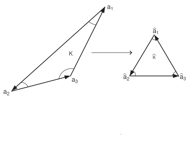
Figure 1: Affine map ${\bf\hat{x}}=\mathcal{F}_{K}{\bf x}$ from $K$ to the reference triangle $\hat{K}$.

Assume that $H({\bf x})$ is a symmetric positive definite matrix on every point ${\bf x}$. Let $\mathcal{M}_{1}({\bf x})=\theta_{1}M_{1}({\bf x})$ where $\theta_{1}$ is to be determined. Here $M_{1}({\bf x})$ is often called the monitor function. Both the monitor function $M_{1}({\bf x})$ and metric tensor $\mathcal{M}_{1}({\bf x})$ play the same role in mesh generation, i.e., they are used to specify the size, shape, and orientation of mesh elements throughout the physical domain. The only difference lies in the way they specify the size of elements. Indeed, $M_{1}({\bf x})$ specifies the element size through the equidistribution condition, while $\mathcal{M}_{1}({\bf x})$ determines the element size through the unitary volume requirement (3.1).

Assume that $H({\bf x})$ is a constant matrix on $K$, denoted by $H_{K}$, then so does $M_{1}({\bf x})$, denoted by $M_{1,K}$. Since $H_{K}$ is a symmetric positive definite matrix, we consider the singular value decomposition $H_{K}=R^{T}\Lambda R$, where $\Lambda=\mbox{diag}(\lambda_{1},\lambda_{2})$ is the diagonal matrix of the corresponding eigenvalues ($\lambda_{1},\lambda_{2}>0$) and $R$ is the orthogonal matrix having as rows the eigenvectors of $H_{K}$. Denote by $F_{K}$ and ${\bf t}_{K}$ the matrix and the vector defining the invertible affine map $\hat{\bf x}=\mathcal{F}_{K}({\bf x})=F_{K}{\bf x}+{\bf t}_{K}$ from the generic element $K$ to the reference triangle $\hat{K}$ (see Figure 1).

Let $M_{1,K}=C_{K}H_{K}$, then $F_{K}=C_{K}^{\frac{1}{2}}\Lambda^{\frac{1}{2}}R$ and $M_{1,K}=F_{K}^{T}F_{K}$. Mathematically, the shape requirement can be expressed as

$$|\hat{\ell}_{i}|=L\,\,\mbox{and}\,\,\cos\hat{\theta}_{i}=\frac{\hat{\ell}_{i+1}\cdot\hat{\ell}_{i+2}}{L^{2}}=\frac{1}{2},\,i=1,2,3,$$

where $L$ is a constant for every element $K$. Together with Theorem 2.1 we have

$$\|\nabla(u-u_{I})\|^{2}_{L^{2}(K)} = \frac{1}{48|K|}\sum_{i=1}^{3}({\bf\ell}_{i+1}\cdot H_{K}{\bf\ell}_{i+2})^{2}|{\bf\ell}_{i}|^{2}$$

$$= \frac{1}{48|K|C_{K}^{2}}\sum_{i=1}^{3}({\bf\ell}_{i+1}\cdot M_{1,K}{\bf\ell}_{i+2})^{2}|{\bf\ell}_{i}|^{2}$$

$$= \frac{L^{4}}{48|K|C_{K}^{2}}\sum_{i=1}^{3}(\cos\hat{\theta}_{i})^{2}|{\bf\ell}_{i}|^{2}$$

$$= \frac{C_{K}\sqrt{\lambda_{1}\lambda_{2}}L^{4}}{192|\hat{K}|C_{K}^{2}}\sum_{i=1}^{3}{\Big{|}}C_{K}^{-\frac{1}{2}}R^{-1}\Lambda^{-\frac{1}{2}}\hat{\ell}_{i}{\Big{|}}^{2}$$

$$= \frac{\sqrt{\lambda_{1}\lambda_{2}}L^{2}}{48\sqrt{3}C_{K}^{2}}\sum_{i=1}^{3}{\Big{|}}\Lambda^{-\frac{1}{2}}\hat{\ell}_{i}{\Big{|}}^{2}$$

$$= \frac{L^{4}}{32\sqrt{3}C_{K}^{2}}{\Big{(}}\sqrt{{\lambda_{1}}/{\lambda_{2}}}+\sqrt{{\lambda_{2}}/{\lambda_{1}}}{\Big{)}}.$$

To satisfy the equidistribution requirement, let

$$\|\nabla(u-u_{I})\|^{2}_{L^{2}(K)}={\Big{(}}\sum\limits_{K\in\mathcal{T}_{h}}e_{K}^{2}{\Big{)}}/N=\epsilon_{1}^{2}/N,$$

where $N$ is the number of elements of $\mathcal{T}_{h}$. Then

$$C_{K}=L^{2}{\Big{(}}\frac{N}{32\sqrt{3}\epsilon_{1}^{2}}{\Big{)}}^{\frac{1}{2}}{\Big{(}}\sqrt{{\lambda_{1}}/{\lambda_{2}}}+\sqrt{{\lambda_{2}}/{\lambda_{1}}}{\Big{)}}^{\frac{1}{2}}=\overline{C}{\Big{(}}\sqrt{{\lambda_{1}}/{\lambda_{2}}}+\sqrt{{\lambda_{2}}/{\lambda_{1}}}{\Big{)}}^{\frac{1}{2}}=\overline{C}{\Big{[}}\frac{\mbox{tr}(H)}{\sqrt{\mbox{det}(H)}}{\Big{]}}^{\frac{1}{2}},$$

where $\overline{C}$ is a constant which depends on the prescribed error and the numbers of elements. Generally speaking, $H({\bf x})$ can not be a constant matrix on $K$ , $M_{1}({\bf x})$ should be the form

$$M_{1}({\bf x})={\Big{[}}\frac{\mbox{tr}(H)}{\sqrt{\mbox{det}(H)}}{\Big{]}}^{\frac{1}{2}}{\Big{[}}H(u){\Big{]}}={\Big{(}}\sqrt{{\lambda_{1}({\bf x})}/{\lambda_{2}({\bf x})}}+\sqrt{{\lambda_{2}({\bf x})}/{\lambda_{1}({\bf x})}}{\Big{)}}^{\frac{1}{2}}{\Big{[}}H(u){\Big{]}},$$

since $M_{1}({\bf x})$ can be modified by multiplying a constant. Note that $\lambda_{1}({\bf x})$ and $\lambda_{2}({\bf x})$ are the corresponding eigenvalue of $H(u)$ at point ${\bf x}$.

To establish $\mathcal{M}_{1}({\bf x})$, the size requirement (3.1) should be used, which leads to

$$\theta_{1}\int_{K}\rho_{1}({\bf x})d{\bf x}=1,$$

where

$$\rho_{1}({\bf x})=\sqrt{\det(M_{1}({\bf x}))}.$$

Summing the above equation over all the elements of $\mathcal{T}_{h}$, one gets

$$\theta_{1}\sigma_{1}=N,$$

where

$$\sigma_{1}=\int_{\Omega}\rho_{1}({\bf x})d{\bf x}.$$

Thus, we get

$$\theta_{1}=\frac{N}{\sigma_{1}},$$

and as a consequence,

$$\mathcal{M}_{1}({\bf x})=\frac{N}{\sigma_{1}}{\Big{[}}\frac{\mbox{tr}(H)}{\sqrt{\mbox{det}(H)}}{\Big{]}}^{\frac{1}{2}}{\Big{[}}H(u){\Big{]}}=\frac{N}{\sigma_{1}}{\Big{(}}\sqrt{{\lambda_{1}({\bf x})}/{\lambda_{2}({\bf x})}}+\sqrt{{\lambda_{2}({\bf x})}/{\lambda_{1}({\bf x})}}{\Big{)}}^{\frac{1}{2}}{\Big{[}}H(u){\Big{]}}.$$

3.2 Metric tensor for the $L^{2}$ norm

Using the expression (2.1) for the $L^{2}$-norm of the linear interpolation error derived by Nadler[30] and the condition (3.1), we have

$$\|u-u_{I}\|^{2}_{L^{2}(K)} = \frac{|K|}{180}{\Big{[}}{\Big{(}}\sum_{i=1}^{3}d_{i}{\Big{)}}^{2}+d_{1}d_{2}+d_{2}d_{3}+d_{1}d_{3}{\Big{]}}$$

$$= \frac{|K|}{180C_{K}^{2}}{\Big{[}}{\Big{(}}\sum_{i=1}^{3}|\hat{\ell}_{i}|^{2}{\Big{)}}^{2}+\sum_{i=1}^{3}{\Big{(}}|\hat{\ell}_{i+1}||\hat{\ell}_{i+2}|{\Big{)}}^{2}{\Big{]}}$$

$$= \frac{L^{4}|K|}{15C_{K}^{2}}=\frac{L^{4}|\hat{K}|}{15C_{K}^{3}\sqrt{\lambda_{1}\lambda_{2}}}=\frac{\sqrt{3}L^{6}}{60C_{K}^{3}\sqrt{\lambda_{1}\lambda_{2}}}.$$

To satisfy the equidistribution requirement, let

$$\|u-u_{I}\|^{2}_{L^{2}(K)}={\Big{(}}\sum\limits_{K\in\mathcal{T}_{h}}e_{K}^{2}{\Big{)}}/N=\epsilon_{0}^{2}/N.$$

Using similar argument with last subsection, we easily get the monitor function

$$M_{0}({\bf x})=\det{\Big{(}}H{\Big{)}}^{-\frac{1}{6}}{\Big{[}}H(u){\Big{]}},$$

and the metric tensor

$$\mathcal{M}_{0}({\bf x})=\frac{N}{\sigma_{0}}\det{\Big{(}}H{\Big{)}}^{-\frac{1}{6}}{\Big{[}}H(u){\Big{]}}$$

for the $L^{2}$ norm.

3.3 Practice use of metric tensors

So far we assume that $H({\bf x})$ is a symmetric positive definite matrix at every point. However this assumption doesn’t hold in many cases. In order to obtain a symmetric positive definite matrix, the following procedure are often implemented. First, the Hessian $H$ is modified into $|H|=R^{T}\,\,\mbox{diag}(|\lambda_{1}|,|\lambda_{2}|)R$ by taking the absolute value of its eigenvalues ([21]). Since $|H|$ is only semi-positive definite, $\mathcal{M}_{0}$ and $\mathcal{M}_{1}$ cannot be directly applied to generate the anisotropic meshes. To avoid this difficulty, we regularize the expression with two flooring parameters $\alpha_{0}>0$ for $\mathcal{M}_{0}$ and $\alpha_{1}>0$ for $\mathcal{M}_{1}$, respectively ([23]). Replace $|H|$ with

$$\mathcal{H}=\alpha_{1}I+|H|,$$

then we get the modified metric tensor

$$\mathcal{M}_{1}({\bf x})=\frac{N}{\sigma_{1}}{\Big{[}}\frac{\mbox{tr}(\mathcal{H})}{\sqrt{\det(\mathcal{H})}}{\Big{]}}^{\frac{1}{2}}{\Big{[}}\mathcal{H}{\Big{]}}.$$ (3.2)

Similarly, replacing $|H|$ with

$$\mathcal{H}=\alpha_{0}I+|H|$$

leads to

$$\mathcal{M}_{0}({\bf x})=\frac{N}{\sigma_{0}}\det{\Big{(}}\mathcal{H}{\Big{)}}^{-\frac{1}{6}}{\Big{[}}\mathcal{H}{\Big{]}}.$$ (3.3)

The two modified metric tensors (3.2) and (3.3) are suitable for practical mesh generation.

4 Numerical experiments

We have elaborated that our metric tensor explores more anisotropic information for a given problem. Then it is crucial to check that whether our metric tensor exhibits better than those without the term

$${\Big{[}}\frac{\mbox{tr}(\mathcal{H})}{\sqrt{\mbox{det}(\mathcal{H})}}{\Big{]}}^{\frac{1}{2}}\quad\mbox{or}\quad{\Big{(}}\sqrt{{\lambda_{1}({\bf x})}/{\lambda_{2}({\bf x})}}+\sqrt{{\lambda_{2}({\bf x})}/{\lambda_{1}({\bf x})}}{\Big{)}}^{\frac{1}{2}}.$$ (4.1)

4.1 Mesh adaptation tool

All the presented experiments are performed by using the BAMG software [22]. Given a background mesh and an approximation solution, BAMG generates the mesh according to the metric. The code allows the user to supply his/her own metric tensor defined on a background mesh. In our computation, the background mesh has been taken as the most recent mesh available.

4.2 Comparisons between two types of metric tensors

Specifically, in every example, the PDE is discretized using linear triangle finite elements. Two serials of adaptive meshes of almost the same number of elements are shown (the iterative procedure for solving PDEs is shown in Figure 2).

Figure 2: Iterative procedure for adaptive mesh solution of PDEs.

The finite element solutions are computed by using the metric tensor of modified Hessian

$$\mathcal{M}_{1}^{m}({\bf x})=\frac{N}{\sigma_{1}}|H|,$$ (4.2)

and the new metric tensor

$$\mathcal{M}_{1}^{n}({\bf x})=\frac{N}{\sigma_{1}}{\Big{[}}\frac{\mbox{tr}(|H|)}{\sqrt{\det(|H|)}}{\Big{]}}^{\frac{1}{2}}|H|.$$ (4.3)

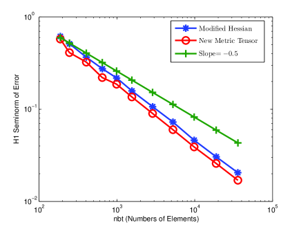
Figure 3: Example 4.1. The $H^{1}$ and $H^{2}$ semi-norms of discretization error are plotted as functions of the number of elements ($nbt$) in (a) and (b), respectively.

Notice that the formulas of the metric tensors involve second order derivatives of the physical solution. Generally speaking, one can assume that the nodal values of the solution or their approximations are available, as typically in the numerical solution of partial differential equations. Then, one can get approximations for the second order derivatives using gradient recovery techniques (such as [40] and [38]) twice or a Hessian recovery technique (using piecewise quadratic polynomials fitting in least-squares sense to nodal values of the computed solution [37]) just once, although their convergence has been analyzed only on isotropic meshes. In our computations, we use the technique [40] twice.

In the current computation, each run is stopped after 10 iterations to guarantee that the adaptive procedure tends towards stability.

Denote by $nbt$ the number of the elements (triangles in 2D case) in the current mesh. The number of triangles or nodes is adjusted when necessary by trial and errors through the modification of the multiplicative coefficient of the metric tensors.

Example 4.1. This example, though numerically solved in $\Omega\equiv(0,1)\times(0,1),$ is in fact one-dimensional:

$$-\kappa\triangle u+\frac{\partial u}{\partial x_{1}} = f,$$

with $f=0$, $u(x_{1}=0,x_{2})=0$, $u(x_{1}=1,x_{2})=1$, and $\frac{\partial u}{\partial n}=0$ along the top and bottom sides of the square (taken from [8]). The exact solution is given by

$$u({\bf x})=\frac{1-e^{\frac{x_{1}}{\kappa}}}{1-e^{\frac{1}{\kappa}}},$$

with a boundary layer of width $\kappa$ at $x_{1}\approx 1$. We have set $\kappa=0.0015$, so that convection is dominant and the Galerkin method yields oscillatory solutions unless the mesh is highly refined at the boundary layer.

Figure 3 (a) compares $H^{1}$ semi-norms of the discretization errors for the two metric tensors. In (b) $H^{2}$ semi-norm of error is computed by the difference between the Hessian of $u$ and the recovered one, which exhibits the quality of meshes to some certain extent.

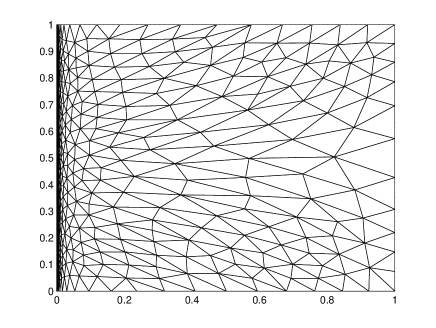
Figure 4: Example 4.2. (a) Anisotropic mesh obtained with the metric tensor $\mathcal{M}_{1}^{m}({\bf x})$: $nbt=4244$, $|e|_{H^{1}}=0.3727$, and $|e|_{H^{2}}=1762$. (b) Anisotropic mesh obtained the metric tensor $\mathcal{M}_{1}^{n}({\bf x})$: $nbt=4243$, $|e|_{H^{1}}=0.2842$, and $|e|_{H^{2}}=1101$.

Example 4.2. We study the Poisson equation (taken from [16])

$$\left\{\begin{array}[]{lll}-\triangle u&=&f,\quad\mbox{in}\quad\Omega\equiv(0,1)\times(0,1),\\ u&=&0,\quad\mbox{on}\quad\partial\Omega,\end{array}\right.$$

where $f$ has been chosen in such a way that the exact solution $u({\bf x})=[1-e^{-\alpha x_{1}}-(1-e^{-\alpha})x_{1}]4x_{2}(1-x_{2})$ and $\alpha$ is chosen to be 1000. Notice that the function $u$ exhibits an exponential layer along the boundary $x_{1}=0$ with an initial step of $\alpha$.

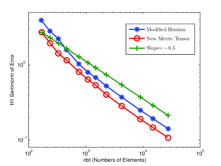
Figure 5: Example 4.2. The $H^{1}$ and $H^{2}$ semi-norms of discretization error are plotted as functions of the number of elements ($nbt$) in (a) and (b), respectively.

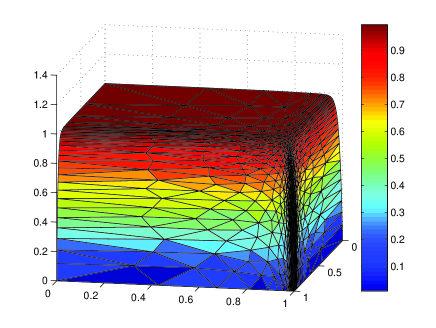
Figure 6: Example 4.3. $\beta=40$, (a) Anisotropic mesh obtained with the metric tensor $\mathcal{M}_{1}^{m}({\bf x})$: $nbt=892$, $|e|_{H^{1}}=0.2581$, $|e|_{H^{2}}=102.0$. (b) Anisotropic mesh obtained with the metric tensor $\mathcal{M}_{1}^{n}({\bf x})$: $nbt=891$, $|e|_{H^{1}}=0.1893$, $|e|_{H^{2}}=57.57$.

Figure 4 contains two meshes obtained by the two different metric tensors (4.2) and (4.3). It is easily seen that the two meshes are obvious different. The former explores more anisotropic features of the solution $u$ than the latter. In other words, the term (4.1) complements more comprehensive information of the exact solution. Figure 5 contains $H^{1}$ and $H^{2}$ semi-norms of error similar to Figure 3.

Example 4.3. Let $\Omega\equiv(0,1)\times(0,1)$, and $u$ be the solution of

$$-\triangle u=\beta(\beta-1)x_{1}^{\beta-2}(1-x_{2}^{2\beta})+2\beta(2\beta-1)x_{2}^{2\beta-2}(1-x_{1}^{\beta})$$

with boundary conditions $u=0$ along the sides $x_{1}=1$ and $x_{2}=1$, and $\partial u/\partial n=0$ along $x_{1}=0$ and $x_{2}=0$ (taken from [8]). The exact solution $u({\bf x})=(1-x_{1}^{\beta})(1-x_{2}^{2\beta})$ exhibits two boundary layers along the right and top sides, the latter being stronger than the former.

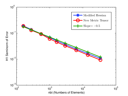
Figure 7: Example 4.3. The $H^{1}$ semi-norms of discretization error are plotted as functions of $nbt$ under the conditions (a) $\beta=5$, (b) $\beta=10$, (c) $\beta=20$, (d) $\beta=40$, respectively.

Figure 6 contains two meshes obtained by the two different metric tensors from solution perspective, where the difference is obvious. This comparison, again, indicates our metric tensor explores more comprehensive anisotropic information of the solution $u$. Figure 7 and Figure 8 contain $H^{1}$ and $H^{2}$ semi-norms of error, respectively, under various parameters $\beta$. We know that the larger the $\beta$ becomes, the more significant the anisotropy of the solution exihibits. Then we can conclude that the more anisotropic the solution is, the more obvious the difference is. In fact, the difference lies on the term (4.1) which indicates our metric tensor explores more comprehensive anisotropic information of the solution when the term varies significantly at different points or elements.

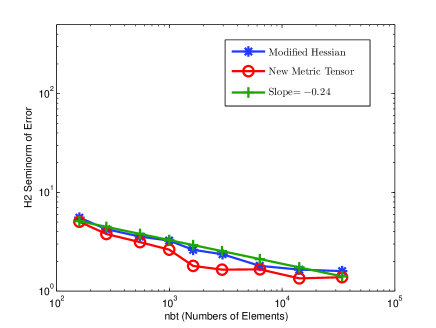
Figure 8: Example 4.3. The $H^{2}$ semi-norms of discretization error are plotted as functions of $nbt$ under the conditions (a) $\beta=5$, (b) $\beta=10$, (c) $\beta=20$, (d) $\beta=40$, respectively.

5 Conclusions

In the previous sections we have developed a new anisotropic mesh adaptation strategy for finite element solution of elliptic differential equations. Note that the new metric tensor $\mathcal{M}_{0}$ for the $L^{2}$ norm is similar to (1.9) ([24]). However, the new metric tensor $\mathcal{M}_{1}$ is essentially different with those metric tensors existed. The difference lies on the term (1.13) which indicates our metric tensor explores more comprehensive anisotropic information of the solution when the term varies significantly at different points or elements. Numerical results also show that this approach is superior to the existing ones to deal with poisson and steady convection-dominated problems.

References

- [1] D. Ait-Ali-Yahia, W. Habashi, A. Tam, M.-G. Vallet, M. Fortin, A directionally adaptive methodology using an edge-based error estimate on quadrilateral grids, Int. J. Numer. Methods Fluids 23 (1996) 673-690.
- [2] T. Apel, G. Lube, Anisotropic mesh refinement in stabilized Galerkin methods, Numer. Math. 74(3) (1996) 261-282.
- [3] R.E. Bank, R.K. Smith, Mesh smoothing using a posteriori error estimates, SIAM J. Numer. Anal. 34 (1997) 979-997.
- [4] R. Becker, An adaptive finite element method for the incompressible Navier-stokes equations on time-dependent domains, Ph.D. thesis, Ruprecht-Karls-Universitt Heidelberg, 1995.
- [5] H. Borouchaki, P.L. George, F. Hecht, P. Laug and E. Saltel, Delaunay mesh generation governed by metric specifications Part I. Algorithms, finite elem. anal. des. 25 (1997) 61-83.
- [6] H. Borouchaki, P.L. George, B. Mohammadi, Delaunay mesh generation governed by metric specifications Part II. Applications, finite elem. anal. des. 25 (1997) 85-109.
- [7] J.U. Brackbill, J.S. Saltzman, Adaptive zoning for singular problems in two dimensions, J. Comput. Phys. 46 (1982) 342-368.
- [8] G. Buscaglia, E. Dari, Anisotropic Mesh Optimization and its Application in Adaptivity, Int. J. Numer. Meth. Eng. 40(22) (1997) 4119-4136.
- [9] W. Cao, On the error of linear interpolation and the orientation, aspect ratio, and internal angles of a triangle, SIAM J. Numer. Anal. 43(1) (2005) 19-40.
- [10] M.J. Castro-Daz, F. Hecht, B. Mohammadi, O. Pironneau, Anisotropic unstructured mesh adaption for flow simulations, Internat. J. Numer. Methods Fluids 25(4) (1997) 475-491.
- [11] L. Chen, P. Sun, J. Xu, Optimal anisotropic meshes for minimizing interpolation errors in -norm, Math. Comp. 76(257) (2007) 179-204.
- [12] E.F. D’Azevedo, R.B. Simpson, On optimal interpolation triangle incidences, SIAM J. Sci. Statist. Comput. 10 (1989) 1063-1075.
- [13] E.F. D’Azevedo, Optimal triangular mesh generation by coordinate transformation, SIAM J. Sci. Stat. Comput. 12 (1991) 755-786.
- [14] E.F. D’Azevedo, R.B. Simpson, On optimal triangular meshes for minimizing the gradient error, Numer. Math. 59 (1991) 321-348.
- [15] A.S. Dvinsky, Adaptive grid generation from harmonic maps on Riemannian manifolds, J. Comput. Phys. 95 (1991) 450-476.
- [16] L. Formaggia, S. Perotto, Anisotropic error estimates for elliptic problems, Numer. Math. 94(1) (2003) 67-92.
- [17] P. Frey, P.L. George, Mesh Generation: Application to Finite Elements, Hermes Science, Oxford and Paris, 2000.
- [18] R.V. Garimella, M.S. Shephard, Boundary layer meshing for viscous flows in complex domain. in: Proceedings of the 7th International Meshing Roundtable, Sandia National Laboratories, Albuquerque, NM, 1998, 107-118.
- [19] P.L. George, F. Hecht. Nonisotropic grids, in: J.F. Thompson, B.K. Soni, N.P. Weatherill, (Eds.), Handbook of Grid Generation, CRC Press, Boca Raton, 1999 20.1-20.29.
- [20] W.G. Habashi, J. Dompierre, Y. Bourgault, D. Ait-Ali-Yahia, M. Fortin, M.-G. Vallet, Anisotropic mesh adaptation: towards user-indepedent, mesh-independent and solver-independent CFD. Part I: general principles, Int. J. Numer. Meth. Fluids 32 (2000) 725-744.
- [21] W.G. Habashi, M. Fortin, J. Dompierre, M.-G. Vallet, Y. Bourgault, Anisotropic mesh adaptation: a step towards a mesh-independent and user-independent CFD, Barriers and challenges in computational fluid dynamics (Hampton, VA, 1996), 99-117, Kluwer Acad. Publ., Dordrecht, 1998.
- [22] F. Hecht, Bidimensional anisotropic mesh generator, Technical Report, INRIA, Rocquencourt, 1997.
- [23] W. Huang. Measuring mesh qualities and application to variational mesh adaptation. SIAM J. Sci. Comput. 26(5) (2005) 1643-1666.
- [24] W. Huang, Metric tensors for anisotropic mesh generation, J. Comput. Phys. 204(2) (2005) 633-665.
- [25] O.P. Jacquotte, A mechanical model for a new grid generation method in computational fluid dynamics, Comput. Meth. Appl. Mech. Eng. 66 (1988) 323-338.
- [26] P. Knupp, L. Margolin, M. Shashkov, Reference jacobian optimization-based rezone strategies for arbitrary lagrangian eulerian methods, J. Comput. Phys. 176 (2002) 93-128.
- [27] R. Kornhuber, R. Roitzsch, On adaptive grid refinement in the presence of internal or boundary layers, IMPACT Comput. Sci. Eng. 2 (1990) 40-72.
- [28] J. Lang, An adaptive finite element method for convection-diffusion problems by interpolation techniques, Technical Report TR 91-4, Konrad-Zuse-Zentrum Berlin, 1991.
- [29] R. Li, T. Tang, and P. Zhang, Moving mesh methods in multiple dimensions based on harmonic maps, J. Comput. Phys. 170(2) (2001) 562-588.
- [30] E.J. Nadler, Piecewise linear approximation on triangulations of a planar region, Ph.D. Thesis, Division of Applied Mathematics, Brown University, Providence, RI, 1985.
- [31] J. Peraire, M. Vahdati, K. Morgan, O.C. Zienkiewicz, Adaptive remeshing for compressible flow computation, J. Comp. Phys. 72(2) (1987) 449-466.
- [32] W. Rachowicz, An anisotropic h-adaptive finite element method for compressible Navier CStokes equations, Comput. Meth. Appl. Mech. Eng. 146 (1997) 231-252.
- [33] J. Remacle, X. Li, M.S. Shephard, and J.E. Flaherty, Anisotropic adaptive simulation of transient flows using discontinuous Galerkin methods, Int. J. Numer. Meth. Eng., 62(7) (2005) 899-923.
- [34] S. Rippa, Long and thin triangles can be good for linear interpolation, SIAM J. Numer. Anal. 29 (1992) 257-270.
- [35] S. Yamakawa and K. Shimada, High quality anisotropic tetrahedral mesh generation via ellipsoidal bubble packing. in: Proceedings of the 9th International Meshing Roundtable, Sandia National Laboratories, Albuquerque, NM, 2000. Sandia Report 2000-2207, 263-273.
- [36] X. Yin, H. Xie, A-posteriori error estimators suitable for moving mesh methods under anisotropic meshes, to appear.
- [37] X. Zhang, Accuracy concern for Hessian metric, Internal Note, CERCA.
- [38] Z. Zhang, A. Naga, A new finite element gradient recovery method: superconvergence property, SIAM J. Sci. Comput. 26(4) (2005) 1192-1213.
- [39] O.C. Zienkiewicz, J. Wu, Automatic directional refinement in adaptive analysis of compressible flows, Int. J. Numer. Meth. Eng. 37 (1994) 2189-2210.
- [40] O.C. Zienkiewicz, J. Zhu, A simple error estimator and adaptive procedure for practical engineering analysis, Int. J. Numer. Meth. Eng. 24 (1987) 337-357.