Entropy production for an interacting quark-gluon plasma

Abstract

We investigate the entropy production within dissipative hydrodynamics in the Israel-Stewart (IS) and Navier-Stokes theory (NS) for relativistic heavy ion physics applications. In particular we focus on the initial condition in a 0+1D Bjorken scenario, appropriate for the early longitudinal expansion stage of the collision. Going beyond the standard simplification of a massless ideal gas we consider a realistic equation of state consistently derived within a virial expansion. The EoS used is well in line with recent three-flavor QCD lattice data for the pressure, speed of sound, and interaction measure at nonzero temperature and vanishing chemical potential ($\mu_{\rm q}=0$). The shear viscosity has been consistently calculated within this formalism using a kinetic approach in the ultra-relativistic regime with an explicit and systematic evaluation of the transport cross section as function of temperature. We investigate the influence of the viscosity and the initial condition, i.e. formation time, initial temperature, and pressure anisotropy for the entropy production at RHIC at $\sqrt{s_{\rm NN}}=130$ GeV. We find that the interplay between effects of the viscosity and of the realistic EoS can not be neglected in the reconstruction of the initial state from experimental data. Therefore, from the experimental findings it is very hard to derive unambiguous information about the initial conditions and/or the evolution of the system.

1 Introduction

Understanding the rich phase structure of quantum chromodynamics for the density-temperature plane is a challenge for theoretical as well as experimental high energy physics. Lattice Monte Carlo simulations have revealed several exciting results over the past decade [1, 2, 3, 4, 5, 6, 7, 8]. At high densities, where the lattice calculations can be performed, effective models of QCD are needed for a theoretical description of this rich phase structure  [9, 10, 11, 12, 13, 14, 15, 16, 17, 18, 19, 20, 21, 22]. From the experimental point of view, heavy-ion collisions are the tool for such investigations. Recent observations at the relativistic heavy-ion collider (RHIC) at Brookhaven National Laboratory (BNL) indicated that the quark-gluon plasma (QGP) created in ultra-relativistic Au + Au collisions is a strongly interacting system. Due to this experimental evidence the QGP can not be satisfactory described by the Stefan-Boltzmann (SB) limit for relativistic noninteracting massless particles, but a realistic equation of state (EoS) has to be used. Recently, we have systematically derived such an EoS within a virial expansion [22]. The recent three-flavor lattice QCD data are described very well for the main thermodynamics quantities, e.g., pressure, entropy density, speed of sound, and interaction measure. Regarding heavy ion collisions, we note that their hydrodynamical modeling plays a crucial role in deducing the experimental findings [23]. Important sources of uncertainty are given by the initial conditions, that are not known precisely. The experimental estimation of the initial energy density has to be taken with care, because it contains simplifications. In fact, Bjorken estimation of the initial energy density at a conservative thermalization time $\tau_{0}=1{\rm fm/c}$ is used assuming a non interacting QGP (i.e. SB equation of state) and a transverse energy distribution per unit of rapidity proper time independent during the evolution of the system [24, 25, 26, 27]. This second assumption allows to avoid any estimation of the lifetime of the deconfined phase but is a strong hypothesis that can lead to changes in the values of the transverse energy density by a factor 2 at times between 1 and 8 fm/c [28]. Therefore, already in the assumption of a non dissipative QGP the estimation of the initial energy density has to be considered with care. The importance of the initial condition has been shown by the large elliptic flow, $v_{2}$, in Au+Au and Cu+Cu collisions at RHIC energies [29, 30, 31, 32, 33, 34, 35, 36, 37, 38, 39, 40]. The centrality, pseudorapidity, and transverse momentum dependences of $v_{2}$ data are described reasonably well by employing the Glauber-type initial conditions and implementing hadronic dissipative effects in ideal hydrodynamic models [41]. However, by replacing the initial conditions from the Glauber model to the ones expected from a color glass condensate, elliptic flow coefficients overshoot the experimental data. This is due to eccentricity larger than the ones in the conventional Glauber model. This discrepancy strongly suggests effects of viscosity in the QGP [42]. A combined investigation of both effects, i.e., viscosity/anisotropy effects and the dependence on the initial condition is needed to understand the competition between these two aspects thoroughly. A measurable quantity that allows such an investigation is the entropy density per unit of rapidity ${\rm d}S/{\rm d}y$. In absence of viscous effects ${\rm d}S/{\rm d}y$ is a conserved quantity and therefore delivers direct information about the initial condition of the system [28], depending on the EoS used. On the other hand, if the shear viscosity, $\eta_{\rm s}$, can not be neglected, ${\rm d}S/{\rm d}y$ increases, and the details of the dynamical evolution become important. Hydrodynamical calculations use a simplified picture for $\eta_{\rm s}$ and for the equation of state. Usually the viscosity to entropy density ratio as temperature independent quantity [42, 43, 44, 45, 46] and/or noninteracting SB-EoS are used [47, 48, 49, 50]. Only recently, calculations including a schematic temperature dependence of $\eta_{\rm s}/s$ in the hadronic phase [51] as well as in the QGP [52] have been performed.

Therefore, a consistent description, where a realistic equation of state as well as the temperature dependent shear-viscosity derived within the same approach is needed to systematically investigate the competition between viscosity and initial condition effects on the hadronic yields. Such a consistent approach is given by the virial expansion, since it allows to derive not only a realistic equation of state for the QGP but also to resolve the whole temperature dependence of the shear viscosity within a kinetic theory [53]. Starting from the results of our model, in this work we will focus on the investigation of the role of the viscosity and the initial conditions for the evolution and finally for the entropy production in heavy-ion collisions. In order to understand the interplay of viscosity, realistic EoS, and initial conditions we consider a $0+1$-dimensional time evolution. This simplified scenario is appropriate for the early longitudinal expansion stage of the collision. Because we focus on the entropy production, which occurs mostly during the early stage of the expansion [44], this approximation is completely justified. In fact, the authors of Ref. [44] claim, that, for a massless ideal gas, the entropy production can be calculated to excellent approximation by assuming boost-invariant longitudinal expansion without transverse flow during this period.

The present work is organized as follows: In Section 2 we briefly recall the basics of the hydrodynamical equation of motion for a shear-viscous, longitudinally boost and transverse translation invariant system. In particular, we discuss how the relativistic perfect fluid (Euler) and the Navier-Stokes equations of motion can be derived from these equations as a special case. In Section 3 we give a brief explanation of the entropy per unit of rapidity in the different scenarios. In Section 4 we present our results by discussing in detail the role of the viscosity and the initial condition, i.e., formation time, initial temperature, and pressure anisotropy for the evolution of the system and the entropy production at RHIC at $\sqrt{s_{\rm NN}}=130$ GeV and the consequences for an improvement of their experimental estimation. The conclusions in Section 5 finalize this work.

2 Boost-invariant hydrodynamics

Relativistic hydrodynamic is based on the local energy-momentum and charge conservation

$$\partial_{\mu}T^{\mu\nu}(x)=0\quad,\qquad\partial_{\mu}n^{\mu}(x)=0\ ,$$ (1)

expressed in terms of the energy-momentum tensor $T^{\mu\nu}(x)$ and of the local charge density $n(x)$. In ideal (Euler) hydrodynamics dissipative effects are neglected. Therefore the energy-momentum tensor and the charge density are given by

$$T^{\mu\nu}_{\rm ID} = (\varepsilon+P)u^{\mu}u^{\nu}-Pg^{\mu\nu}$$ (2)

$$n^{\mu}_{\rm ID} = nu^{\mu},$$ (3)

where $\varepsilon$ and $P$ are the energy density and the pressure, respectively; $u^{\mu}$ is the flow four-velocity normalized to $u^{\mu}u_{\mu}=1$ using the standard metric tensor $g^{\mu\nu}={\rm diag}(1,-1,-1,-1)$. The simplest extension to a dissipative regime is the introduction of additive corrections linear in flow and temperature gradients [47], the so-called Navier-Stokes (NS) approximation

$$\delta T^{\mu\nu}_{\rm NS} = \eta_{\rm s}(\nabla^{\mu}u^{\nu}+\nabla^{\nu}u^{\mu}-\frac{2}{3}\Delta^{\mu\nu}\partial^{\alpha}u_{\alpha})+\zeta\Delta^{\mu\nu}\partial^{\alpha}u_{\alpha},\quad$$ (4)

$$\delta n^{\mu}_{\rm NS} = \kappa_{\rm q}\left(\frac{nT}{\varepsilon+p}\right)^{2}\nabla^{\mu}\left(\frac{\mu}{T}\right),\quad$$ (5)

$$\Delta^{\mu\nu} \equiv g^{\mu\nu}-u^{\mu}u^{\nu}\qquad{\rm and}\qquad\Delta^{\mu}\equiv\Delta^{\mu\nu}\partial_{\nu},$$ (6)

where $\zeta$ indicates the bulk viscosity, and $\kappa_{\rm q}$ is the heat conductivity of the system. The hydrodynamic equations in NS approximation can be derived from a general non-equilibrium theory, the on-shell covariant transport [54, 55]. The relativistic NS equations are parabolic and therefore acausal. The solution formulated by Israel and Stewart (IS) [56, 57] transforms the NS equations into relaxation equations for the shear stress, $\pi^{\mu\nu}$, bulk pressure, $\Pi$, and heat flow, $q^{\mu}$. The corrections are given by

$$\delta T^{\mu\nu}\equiv\pi^{\mu\nu}-\Pi\Delta^{\mu\nu},\quad\delta n^{\mu}\equiv-\frac{n}{\varepsilon+p}q^{\mu}$$ (7)

with

$$u_{\mu}q^{\mu}=0,\quad u_{\mu}\pi^{\mu\nu}=u_{\mu}\pi^{\nu\mu}=0.$$ (8)

The original derivation of the IS equations is not a systematically controlled approximation of the transport theory because it is not an expansion in some small parameter. In Ref. [57] a quadratic ansatz for the deviation from local equilibrium has been employed. Nevertheless, in Ref. [58] a new method for deriving the fluid-dynamical equations has been proposed. In this novel approach the equation for the dissipative currents are directly obtained from the definitions of the currents. We note that, although these equations of motion are formally identical to the original IS equations, the coefficients are different. For a detailed overview of the IS theory see Ref. [47]. Here we remark that the starting point is given by an entropy current that includes terms up to quadratic order in dissipative quantities. These terms are expressed - using Landau frame notation - by the same coefficients $\alpha_{0},\alpha_{1},\beta_{0},\beta_{1},\beta_{2},$ that encode additional transport properties. In particular, the set $\{\beta_{i}\}$ describes the relaxation times for dissipative quantities as

$$\tau_{\Pi}=\zeta\beta_{0}\ ,\qquad\tau_{\rm q}=\kappa_{\rm q}T\beta_{1}\ ,\qquad\tau_{\pi}=2\eta_{\rm s}\beta_{2}\ .$$ (9)

The NS theory is recovered when all these coefficients are set to zero $\beta_{0}=\beta_{1}=\beta_{2}=\alpha_{0}=\alpha_{1}=0$.

In the following we focus on a viscous, longitudinally boost-invariant system with transverse translation invariance and vanishing bulk viscosity. As a boost-invariant system we consider a system with a longitudinal scaling flow, $\vec{v}=(0,0,z/t)$, and where all scalar quantities are independent of the spatial rapidity, defined by

$$\eta=\frac{1}{2}\ln[(t+z)/(t-z)].$$ (10)

If the initial densities are assumed to depend on $t$ and $z$ only through the Bjorken (longitudinal) proper time

$$\tau=\sqrt{t^{2}-z^{2}},$$ (11)

the expansion will evolve such that densities remain independent of $\eta$. The $v_{z}$ will retain the scaling form $v_{z}=z/t$ [59]. Accordingly, all vector and tensor quantities can be obtained from their values at $\eta=0$ by an appropriate Lorentz boost. Because of the symmetries of the system, i.e., longitudinal boost invariance, axial symmetry in the transverse plane and $\eta\to-\eta$ reflection symmetry, the heat flow is zero everywhere. Furthermore, only the viscous corrections to the longitudinal, $\pi_{\rm L}$, and transverse pressure, $\pi_{\rm T}$, i.e., $\pi_{\rm zz}$ and $\pi_{\rm xx}=\pi_{\rm yy}$ components of the shear stress tensor evaluated in the local rest frame, are non-vanishing. The choice to neglect bulk viscosity is sensible since shear viscosity is expected to dominate at RHIC. The absence of heat flow as well as bulk viscosity leads to

$$\tau_{\Pi}=\tau_{\rm q}=0.$$ (12)

Only the relaxation time, $\tau_{\pi}$, enters in the equation of motion. With these assumptions the equations of motion can be written as

$$\dot{n}+\frac{n}{\tau} = 0$$ (13)

$$\dot{\varepsilon}+\frac{\varepsilon+p}{\tau} = -\frac{\pi_{\rm L}}{\tau}$$ (14)

$$\tau_{\pi}\dot{\pi}_{\rm L}+\pi_{\rm L}\left[1+\frac{\tau_{\pi}}{2\tau}+\frac{\eta_{\rm s}T}{2}\dot{\left(\frac{\tau_{\pi}}{\eta_{\rm s}T}\right)}\right] = -\frac{4\eta_{\rm s}}{3\tau}$$ (15)

$$\pi_{\rm T} = -\frac{\pi_{\rm L}}{2}\ ,$$ (16)

where the ’dot’ denotes ${\rm d}/{\rm d}\tau$. This special case is a useful approximation to the early longitudinal expansion stage of a heavy ion collision for observables near midrapidity $\eta\approx 0$ [47]. Obviously, Eq.(13) describes particle conservation and can be solved as

$$n(\tau)=\frac{\tau_{0}\,n(\tau_{0})}{\tau}.$$ (17)

In Ref. [47] these equation of motions have been studied with the assumption of an ideal massless equation of state. Because of this oversimplification the density equation (13) decouples entirely leading to two coupled equations for the equilibrium pressure and the viscous correction, $\pi_{\rm L}$. For two limiting scenarios, - for the scale invariant case of a constant shear viscosity to entropy density ratio, $\eta_{\rm s}/s$, and for dynamics driven by a constant cross section - analytic approximate solutions can be found. However, we focus on a realistic equation of state and therefore the limitation of a massless ideal system must be neglected. We then use the results of the virial expansion for the equation of state [22] as well as for the shear viscosity [53], where, within a kinetic approach in the ultra relativistic regime, the transport cross section as function of the temperature has been consistently evaluated. Therefore, we use the relaxation time $\tau_{\pi}$ with the ultra relativistic assumption. As in Ref. [57] we obtain

$$\tau_{\pi}=\frac{3\eta_{\rm s}}{2p}.$$ (18)

Note that in this way we can systematically investigate the interplay of different effects - realistic equation of state, dissipation, dependence on the initial condition- in the same framework. In the following we briefly discuss these different scenarios in detail and give the analytic solution of the equation of motion, where possible.

2.1 Ideal Hydrodynamics

The simplest case is that the system does not suffer any dissipative effects. Accordingly, we have

$$\tau_{\pi}^{\rm ID}=\eta_{\rm s}^{\rm ID}=0,$$ (19)

and the relevant equation of motion is

$$\dot{\varepsilon}+\frac{\varepsilon+p}{\tau}=0.$$ (20)

This automatically follows from $\pi_{\rm L}=\pi_{\rm T}=0$. Equation (20) is equivalent to

$$\frac{{\rm d}}{{\rm d}\tau}(s\tau)=0,$$ (21)

which indicates that $s\tau$ is a conserved quantity. This conservation law is broken if dissipative effects emerge. Thus the entropy density evolution is given by

$$s(\tau)=\frac{s_{0}\tau_{0}}{\tau},\qquad{\rm with}\quad s_{0}=s(\tau_{0}).$$ (22)

Consequently, using an EoS a solution of the equation of motion (EoM) can be given without explicitly solving Eq.(20). A formal solution for the energy density evolution $\varepsilon=\varepsilon(\tau)$ has the form

$$\varepsilon(\tau)=\varepsilon_{0}\left(\frac{\tau_{0}}{\tau}\right)^{1+c_{0}^{2}},\qquad{\rm with}\quad c_{0}^{2}=\frac{p}{\varepsilon}\quad{\rm and}\quad\varepsilon_{0}=\varepsilon(\tau_{0}).$$ (23)

This results from the separable structure of the EoM, or, more precisely, because it is an exact differential equation. Obviously, this formal solution holds also for the Stefan-Boltzmann limit, where $c_{0}^{\rm SB}=1/3$ coinciding with the sound velocity defined by

$$c_{\rm s}^{2}=\frac{\partial P}{\partial\varepsilon}=\varepsilon\frac{\partial c_{0}^{2}}{\partial\varepsilon}+\frac{P}{\varepsilon}.$$ (24)

This leads to the well known power law $\varepsilon^{\rm SB}(\tau)\propto(\tau_{0}/\tau)^{-4/3}$. In general for a realistic EoS an explicit solution, $\varepsilon(\tau)$, is not possible, because the $c_{0}$ itself is a function of $\varepsilon$. However, for the QGP, the ratio pressure to energy density can be parameterized using the phenomenological ansatz [60]

$$\frac{p}{\varepsilon}=\frac{1}{3}\left(C-\frac{A}{1+B\varepsilon}\right),$$ (25)

that provides a good fit to the lattice data in the interval $1.3\leq\varepsilon^{1/4}/({\rm GeV/fm^{3}})^{1/4}\leq 6$ with $C=0.964(5)$, $A=1.16(6)$ and $B=0.26(3){\;\rm fm^{3}/GeV}$ [8]. Using this parametrization we can explicitly solve the equation of motion (20) as

$$F(\varepsilon)=F_{0}\frac{\tau_{0}}{\tau}\qquad{\rm with}\quad F_{0}=F(\varepsilon_{0}).$$ (26)

The solving polynomial function is given by

$$F(\varepsilon)=\varepsilon^{\frac{1}{D}}(\varepsilon+\omega)^{\frac{3}{C+3}-\frac{1}{D}}$$ (27)

with the constants,

$$D = \frac{C}{3}+1-A$$ (28)

$$\omega = 1-\frac{3A}{C+3}=\frac{D}{B(1+C/3)}.$$ (29)

naturally, setting $A=0$ and $C=1$ - and $D=4/3$ and $\omega=1$ - the evolution in the SB-limit is recovered.

2.2 Navier-Stokes

As mentioned previously, the simplest way to introduce dissipative effects is considering the linear Navier-Stokes equations. In this approximation all relaxation times are vanishing and consequently the equations for the energy density evolution and the viscous correction, $\pi_{\rm L}$, completely decouple

$$\dot{\varepsilon}+\frac{\varepsilon+p}{\tau} = \frac{4}{3}\frac{\eta_{\rm s}}{\tau^{2}},$$ (30)

$$\pi_{L} = -\frac{4\eta_{s}}{3\tau}.$$ (31)

The NS equation of motion (30) can be reduced to an exact differential equation. Formally, using the same notation as before, we can write

$$\varepsilon(\tau)=\varepsilon_{0}\left(\frac{\tau_{0}}{\tau}\right)^{1+c_{0}^{2}}H_{\rm NS}(\eta_{\rm s}),$$ (32)

where the dissipative correction, $H_{\rm NS}$, is given by

$$H_{\rm NS}(\eta_{\rm s})=\exp\left\{-\frac{4}{3}\int_{\tau_{0}}^{\tau}{\rm d}\tau^{\prime}\frac{\partial\eta_{\rm s}}{\partial\varepsilon}\frac{1}{\tau^{\prime 2}}\right\},$$ (33)

Eq. (33) corresponds to the integration factor needed to transform the NS equation motion in to an exact differential equation. This structure can be found as well in Ref. [61], where, by assuming for the evolution of the viscosity

$$\eta_{\rm s}^{\rm nl}=C_{\rm NS}\;\varepsilon\tau+C_{\rm nl}\;\varepsilon/\tau,$$ (34)

non local corrections governed by the parameter, $C_{\rm nl}$, have been included. With this analytic form for the viscosity the dissipative correction given by $H_{\rm NS}$ can be easily calculated, and one finds

$$\varepsilon^{\rm nl}(\tau) = \varepsilon(\tau_{0})\left(\frac{\tau_{0}}{\tau}\right)^{(1+c_{0}^{2}-(4/3)C_{\rm NS})}H_{\rm NS}^{\rm nl}(\eta_{\rm s}^{\rm nl})$$ (35)

$$= \varepsilon(\tau_{0})\left(\frac{\tau_{0}}{\tau}\right)^{(1+c_{0}^{2}-(4/3)C_{\rm NS})}\exp\left\{\frac{2C_{\rm nl}}{3}\left(\frac{1}{\tau_{0}^{2}}-\frac{1}{\tau^{2}}\right)\right\},$$

as shown in [61] for massless non-interacting particles, i.e., setting $c_{0}^{2}=1/3$. This assumption for the viscosity means that an additional coupled equation for the time evolution of $\eta_{\rm s}$ has been implicitly added in the investigation. This is not our strategy, because we have completely determined the shear viscosity in a systematic way, and we can also calculate the time evolution without further assumptions. In fact, the EoS and the knowledge of the dependence of the viscosity on the thermodynamics quantities,.i.e., on the energy density, $\varepsilon$ [22, 53], allows us to find a coupled system of equations for the NS scenario as well as in the general case. Therefore, by finding a parametrization of $\eta_{\rm s}=\eta_{\rm s}(\varepsilon)$, we are able to give an analytic solution calculating $H_{\rm NS}^{\rm Vir}(\eta_{\rm s})$. We note in passing that in this way the equation for the energy density and for the viscous correction for the pressure decouple. However, we prefer to directly solve the equations of motion without introducing any parametrization for the viscosity.

3 Entropy production

Now we define the basic observable investigated in this study, and consider its different evolution in the different scenarios. In the rest of the paper, the subscript ’0’ refers to the value of quantities at the initial time, $\tau_{0}$.

The most natural quantitative measure of dissipative effects is the entropy production. An often used quantity is the entropy per unit rapidity

$$\frac{{\rm d}S}{{\rm d}y}=\tau\int{\rm d}^{2}x_{\rm T}\,s=\tau A_{\rm T}s,$$ (36)

where $A_{\rm T}$ is the transverse area of the system. This quantity highlights several aspects of the QGP because the final entropy production can be measured [28] and, additionally, it is sensitive to the dissipative properties of the system. In ideal hydrodynamics, the entropy per unit rapidity is evidently a constant of the evolution. By the experimental measurement of the entropy production at the final time $\tau_{\rm f}$ one can conclude the initial condition as

$$\frac{{\rm d}S^{\rm ID}}{{\rm d}y}(\tau_{\rm f})=\frac{{\rm d}S^{\rm ID}}{{\rm d}y}(\tau_{0})=\tau_{0}A_{\rm T}s_{0}.$$ (37)

In the NS scenario and in the IS regime, dissipative effects determine an enhancement of the entropy production. This viscous correction depends of course on the initial conditions, specifically on the formation time and initial energy density as usual, but in general also on the initial pressure anisotropy. Therefore, the most natural choice for the initial conditions are the initial entropy density, $s_{0}$, and the initial ratio of viscous longitudinal shear and equilibrium pressure, $\xi_{0}$, defined as

$$\xi_{0}\equiv\frac{{\pi_{\rm L}}_{0}}{p_{0}}.$$ (38)

A useful equivalent measure is the pressure anisotropy coefficient

$$R_{0}\equiv\frac{{p_{\rm L}}_{0}}{{p_{\rm T}}_{0}}=\frac{1+\xi_{0}}{1-\xi_{0}/2}\ ,$$ (39)

which is the ratio of the transverse and longitudinal pressures ${p_{\rm T}}_{0}\equiv p-{\pi_{\rm L}}_{0}/2$, ${p_{\rm L}}_{0}\equiv p_{0}+{\pi_{\rm L}}_{0}$. Evidently, $\xi_{0}=0$ indicates central collisions, where pressure anisotropy can not develop, whereas peripheral collisions lead to larger $|\xi_{0}|$.

We have shown in Section 2.1 that in ideal hydrodynamics the viscous corrections to the pressure always vanish. In this scenario the anisotropy is unity and

$$R_{0}^{\rm ID}=1\qquad{\rm and}\quad\xi_{0}^{\rm ID}=0.$$ (40)

are automatically fulfilled.

As explained in Section 2.2, in the NS approximation the evolution of the energy density and of the viscosity are uniquely determinated by Eq.(30). Therefore, the initial anisotropy is automatically fixed by the initial condition over the entropy density $s_{0}$ and any dependence on $\xi_{0}$ (or $R_{0}$) vanishes. In IS the dependence on the initial pressure anisotropy emerges and thus in this scenario we need it as a second initial condition. Additionally, Eq.(36) shows that the entropy production is proper time dependent. Therefore, the final proper time $\tau_{\rm f}$ enters as an important parameter to describe the experimental data.

4 Application to 130 GeV Au + Au collisions

As mentioned in the previous section the entropy production allows – in principle – to quantify the dissipative effects. Furthermore, experimental results are available for Au + Au collision at RHIC at $\sqrt{s_{\rm NN}}=130$ GeV [28], where the final entropy production per unit rapidity is 4501 with an uncertainty of about $10\%$. In the following we attempt to categorize which (dissipative) effects and initial conditions are compatible with these experimental findings. As in Ref. [28] we compare the experimental value to the hydrodynamic ${\rm d}S/{\rm d}y$ as a function of the initial energy density, $\varepsilon_{0}$. We emphasize that $\varepsilon_{0}$ is strongly dependent on the choice of the formation time, $\tau_{0}$. In Ref. [28] the authors use a conservative formation time, $\tau_{0}=1$ fm/c.

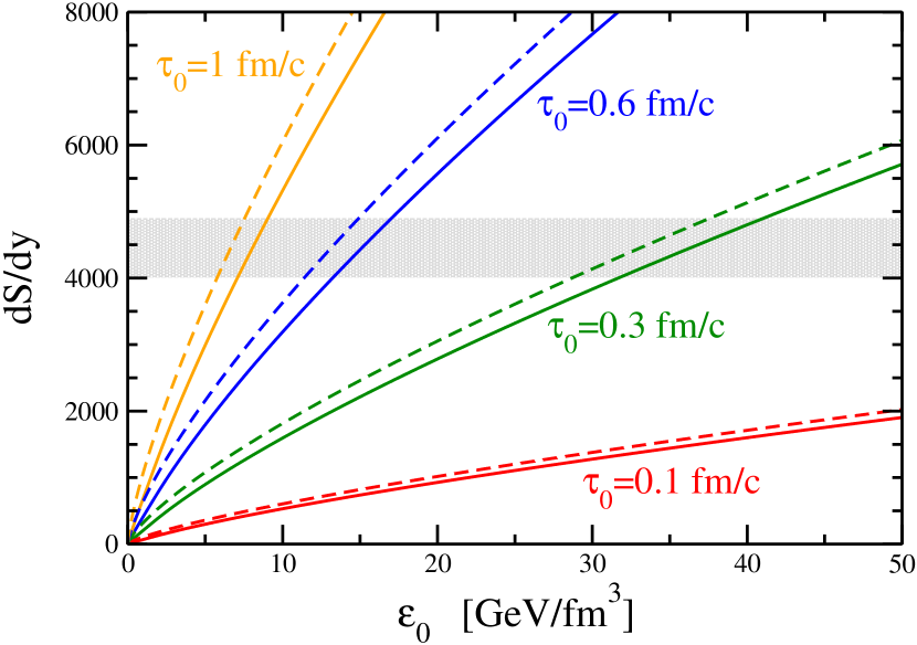
Figure 1: (Color online) The entropy per unit rapidity is displayed as a function of the initial energy density $\varepsilon_{0}$ for the QGP using a realistic EoS [22] (solid lines) in comparison to the SB limit (dashed lines) for different formation times, $\tau_{0}=0.1,\,0.3,\,0.6,\,1$ fm/c (red, green, blue and orange lines). The horizontal band shows the final-state entropy extracted from experiment. Hydrodynamic simulations typically have energy densities between 10 and 15 GeV/fm³ and formation times of about 0.6 fm/c.

Our aim is the investigation of the role of all initial conditions and therefore the explicit dependence on the formation time has to be considered. As a first step, we focus on the importance to use a realistic EoS, in order to clarify the amount and the behavior of the effects that a realistic EoS generates in the experimental observables. In Fig. 1 the entropy per unit rapidity is shown as a function of the initial energy density, $\varepsilon_{0}$, for the QGP using the realistic EoS of [22] (solid lines ) for various formation times. In following we refer to such calculation as non dissipative scenario (ND). For comparison, we indicate by the dashed line the SB-limit for the same initialization times using the same color coding. The horizontal band shows the final-state entropy extracted from experiment. Evidently, too fast thermalization times, $\tau_{0}=0.1$ fm/c and $\tau_{0}=0.3$ fm/c, lead to an unreasonably high initial energy density. Hydrodynamic simulations typically use formation times about 0.6 fm/c, which corresponds to the blue lines of Fig. 1. The corresponding results for the entropy in our calculation suggests energy densities between 10 and 15 GeV/fm³, which is in agreement with ideal hydrodynamic simulations. We remark here that for this typical hydrodynamic formation time as well as for the conservative one, $\tau_{0}=1$ fm/c, used in several evaluations (extrapolations) of measured experimental data, the difference between SB and realistic EoS is not negligible. Therefore, the precise determination of the initial conditions is necessary for a good description of the evolution of the system.

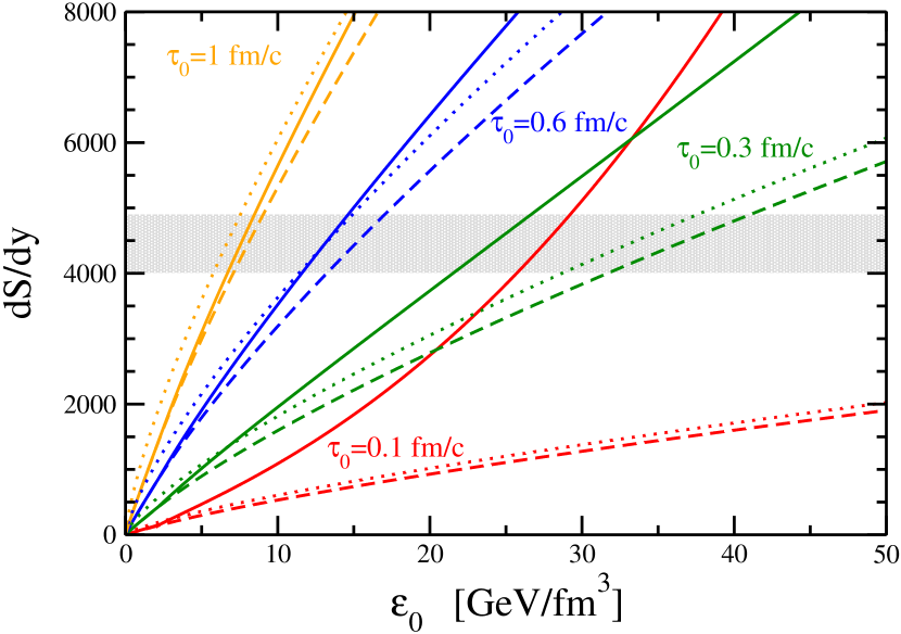
Figure 2: (Color online) The entropy per unit rapidity is picted as a function of the initial energy density, $\varepsilon_{0}$, for a dissipative realistic QGP [22, 53] within the NS approximation (solid lines) in comparison to the ND results (dashed lines) and the SB limit (pointed line) for different formation times, $\tau_{0}=0.1,\,0.3,\,0.6,\,1$ fm/c (red, green, blue and orange lines). The horizontal band shows the final-state entropy extracted from experiment.

In this context, an implementation of the viscosity effect have a larger impact.

Because of the dissipative effects in the QGP, the entropy density per unit rapidity is an increasing function of the proper time. Following [44] we assume that the final entropy is mostly produced in the early phases of the collisions, and then we can neglect the contribution of the hadronic phase. Therefore the final time, $\tau_{\rm f}$, is automatically fixed, namely as the time when the energy density of the system is equal to the critical energy density,

$$\varepsilon(\tau_{\rm f})=\varepsilon(T_{\rm c}).$$ (41)

Because in the NS approximation the initial viscosity of the system is completely determined by the initial energy density, we can directly compare the results for the entropy per unit rapidity for the non dissipative system shown before with the ones from the NS equation of motions. Using the same color coding as before, we show in Fig. 2 the entropy per unit rapidity as a function of the initial energy density $\varepsilon_{0}$ for the dissipative QGP [22, 53] within the NS approximation (solid lines) for various formation times in comparison with the non dissipative and SB calculations. For all formation times one observes an enhancement of the entropy production by the NS viscous corrections in comparison to the ND results. For $\tau_{0}=1$ fm/c and $\tau_{0}=0.6$ fm/c we find moderate corrections, that seem to recover the results of the SB ideal fluid shown in Fig. 1. In particular, for $\tau_{0}=0.6$ fm/c, the effect of a realistic equation of state and the linear (NS) viscous terms compensate also quantitatively each other. For the faster thermalization scenarios, $\tau=0.3$ fm/c and $\tau=0.1$ fm/c, the enhancement is very significant and allows to describe the experimental finding for the entropy per unit of rapidity using smaller – but nevertheless high – $\varepsilon_{0}$ of about 20 GeV/fm³ and 25 GeV/fm³ respectively. The formation time, $\tau_{0}$, indicates an atypical behavior, not only because of the pronounced enhancement of the entropy production, but primarily because of the change from a concave to a convex function in ${\rm d}S/{\rm d}y(\varepsilon_{0})$. This can be a hint that results in NS approximation with small formation time have to be questioned. Deciding this question, one has to consider the full IS equations of motion for the entropy production.

As explained in Section 3 the initial conditions for the IS equation of motion are not completely fixed by the initial energy density of the system because of the additional explicit anisotropy of the system. Therefore, one has a family of solutions labeled by the anisotropy coefficient, $\xi_{0}$, as additional parameter. For each formation time, we calculate, for different values of the initial anisotropy, the entropy production at $T=T_{\rm c}$ as function of the initial energy density. We use $\xi_{0}=0$, $\xi_{0}=-0.5$, and $\xi_{0}=-1$, which correspond to the values for the anisotropy coefficient of $R_{0}=1$, $R_{0}=2/3$, and $R_{0}=0$, respectively. We prefer to concentrate on two limiting cases, $\tau_{0}=0.1$ fm/c and $\tau_{0}=1$ fm/c.

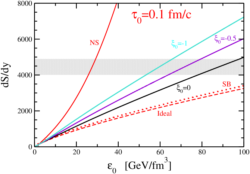
Figure 3: (Color online) The entropy per unit rapidity is depicted as a function of the initial energy density, $\varepsilon_{0}$, for a dissipative realistic QGP [22, 53] at $\tau_{0}=0.1$ fm/c within the IS approach for different values of the initial pressure anisotropy, $\xi_{0}=0,-1,-2,-3$ (black, turquoise, violet and brown solid line respectively) in comparison to the NS approximation (red solid line), the ND scenario (dashed red line) and the SB limit (dotted red line). The horizontal band shows the final-state entropy extracted from experiment.

In Fig. 3 we show the entropy per unit rapidity as a function of the initial energy density $\varepsilon_{0}$ with the formation time $\tau_{0}=0.1$ fm/c within the IS approach. The different values of the initial pressure anisotropy $\xi_{0}=0,-0.5,-1$ are displayed as black, violet and turquoise lines, respectively.

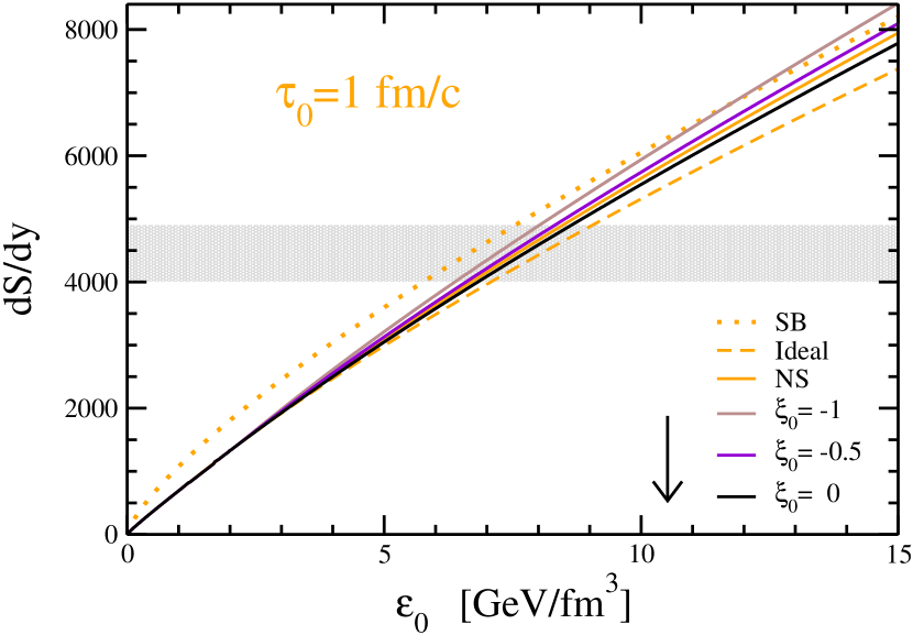
Figure 4: (Color online) The entropy per unit rapidity is displayed as a function of the initial energy density, $\varepsilon_{0}$, for a dissipative realistic QGP [22, 53] at $\tau_{0}=1$ fm/c within the IS approach for different values of the initial pressure anisotropy, $\xi_{0}=0,-1,-2,-3$ (black, turquoise, violet and brown solid line respectively) in comparison to the NS approximation (orange solid line) and the ND scenario (dashed orange line) and the SB limit (dotted orange line).The horizontal band shows the final-state entropy extracted from experiment.

For comparison we added the corresponding results within the NS approximation (red solid line), the ND scenario (dashed red line) and the SB limit (dotted red line). The experimental result is located within the horizontal band in Fig. 3. Already at vanishing anisotropy the deviation from the previous results is evident in the whole energy range. the difference to the non dissipative scenario are small for low initial energy density, $\varepsilon\geq 10$ GeV/fm³. By increasing the anisotropy of the system, the entropy production also increases. For all values of $\xi_{0}$ we observe a linear relation between ${\rm d}S/{\rm d}y$ and $\varepsilon_{0}$. Nevertheless, we reject such a fast formation time for two reasons: not only does the NS formulation not allow $\tau_{0}=0.1$ fm/c, but also at extremely high initial anisotropy $\xi_{0}=-1$, that corresponds to the limiting case with the tranverse pressure only, high values of the initial energy density are needed to reproduce the experimental entropy production. That makes this scenario unlikely. The contrary situation is given by a conservative formation time, $\tau_{0}=1$ fm/c.

In this case Fig. 4 shows the results for the entropy per unit rapidity as a function of the initial energy density $\varepsilon_{0}$ within the IS approach for the same values of $\xi_{0}$ as before. Again, we compare to the corresponding results in the NS approximation (orange solid line), the ND scenario (dashed orange line) and the SB limit (dotted orange line). We note the same qualitative behavior as for the small formation time (Fig. 3): by increasing the anisotropy of the system, the entropy production also increases. In particular, we find an initial energy density between $\varepsilon_{0}\approx 7-9\;{\rm GeV/fm}^{3}$, that is larger than experimental estimation in Ref. [62] of about $\varepsilon_{0}\approx 4-5\;{\rm GeV/fm}^{3}$. This is not surprising, because the experimental measure is based on very simplified and strong assumptions, that do not give a realistic description of the system. This suggests that the estimation procedures have to be improved because of the effects of the final proper time $\tau_{\rm f}$, the viscosity and the anisotropy can not be neglected. To be more quantitative we can extract from the experimental estimation of the final entropy the initial energy density for different formation times in the different scenarios. In this way we can compare the (typical experimental) values, $\varepsilon^{\rm SB}_{0}$, obtained using the ideal Bjorken expansion, i.e., the SB limit, with the values $\varepsilon^{\rm ND}_{0}$, $\varepsilon^{\rm NS}_{0}$ and $\varepsilon^{\rm IS}_{0}$ in the ND scenario, in the NS and IS theory respectively. Evidently, for the IS calculation, non only the parametric dependence on the formation time $\tau_{0}$, but also on the initial pressure anisotropy $\xi_{0}$ has been considered. The results are summarized in Tab. 1 and Tab 2, where the deviation from the standard SB estimation of the ND, NS and IS calculation is listed.

Table 1: Results for the deviation from the SB estimation of the initial energy density in the ND and NS scenario

$\tau_{0}$	$\varepsilon^{\rm SB}_{0}$	$\varepsilon^{\rm ND}_{0}/\varepsilon^{\rm SB}_{0}$	$\varepsilon^{\rm NS}_{0}/\varepsilon^{\rm SB}_{0}$
${\rm[fm/c]}$	${\rm[GeV/fm^{3}}]$
0.1	143.10	1.05	0.20
0.3	33.07	1.10	0.73
0.6	13.12	1.15	0.99
1.0	6.64	1.21	1.14

Table 2: Results for deviation from the SB estimation of the initial energy density in the IS scenario

$\tau_{0}$	$\varepsilon^{\rm SB}_{0}$	$\varepsilon^{\rm IS}_{0}/\varepsilon^{\rm SB}_{0}$,	$\varepsilon^{\rm IS}_{0}/\varepsilon^{\rm SB}_{0}$,	$\varepsilon^{\rm IS}_{0}/\varepsilon^{\rm SB}_{0}$,
${\rm[fm/c]}$	${\rm[GeV/fm^{3}}]$	$\xi_{0}=0$	$\xi_{0}=-0.5$	$\xi_{0}=-1$
0.1	143.10	0.62	0.50	0.41
0.33	3.07	0.9	0.80	0.72
0.6	13.12	1.02	0.99	0.93
1.0	6.64	1.16	1.12	1.08

For small formation times ($\tau_{0}=0.1$ fm/c and $\tau_{0}=0.3$) the effects of the relativistic equations are almost negligible, i.e. lower then $10\%$. However, dissipative effects are to be included, because the viscosity leads to an deviation between $30\%$ and $80\%$ in the NS scenario and between $40\%$ and $60\%$ in the IS scenario. Only for central collisions ($\xi_{0}=0$) the deviation in the formation time $\tau_{0}=0.3$ fm/c is maybe reasonable ($10\%$), although, in this case, the assumption leads to an unlikely large initial energy density. Therefore, such small formations time have to be rejected. For $\tau_{0}=0.6$ fm/c, often used in hydrodynamical calculations, we note that the viscous effects completely compensate the correction of the realistic EoS in the NS scenario and in the IS theory for non peripheral collisions. Thus, in this case, using the Bjorken expansion can be justified. For the conservative formation time, $\tau_{0}=1$ fm/c, the effects of the realistic EoS are more important, about $20\%$, and can not be compensated by the inclusion of NS viscous corrections. Therefore, it is not surprising, that also in central collisions in the IS scenario the deviation is also sizable. For more peripheral collisions the SB limit seems to lead to a more or less satisfactory approximation (about $8\%$) for the IS calculations. Nevertheless, from this discussion it is evident, that the use of the Bjorken expansion for the evaluation of the initial energy density, without considerations of interplay between formation time, viscosity, and the centrality of the collisions can be very questionable. Additionally, the quite satisfactory agreement between IS hydrodynamics calculations and the transport ones within the cascade BAMPS for small $\eta_{\rm s}$ [63, 64] also remarks the validity of the IS scenario.

5 Conclusions

In this work we have discussed the importance of the initial condition and the role of the viscosity for the evolution of the fireball of heavy-ion collisions. We have used a realistic EoS derived within a virial expansion [22], that is in line with recent three-flavor lattice QCD data [8]. The shear viscosity has been consistently calculated within this formalism using a kinetic approach in the ultra-relativistic regime with an explicit and systematic evaluation of the transport cross section as a function of temperature [53]. We explicitly considered different scenarios: ideal hydrodynamic, dissipative effects in the Navier-Stokes as well as in the Israel-Stewart formalism, from conservative to very fast equilibration dynamics. We choose the parameter of these studies in order to describe the experimental findings of the entropy production for Au + Au collision at RHIC at $\sqrt{s_{\rm NN}}=130$ GeV. The assumption of a fast equilibration would require unreasonably high values of the initial energy density. With the conservative ($\tau_{0}=1$ fm/c) and the typical hydrodynamical ($\tau_{0}=0.6$ fm/c) formation times the initial energy density needed to reproduce the final entropy is more in line with the experimental estimations. In these scenarios, the interplay between effects of the viscosity and of the realistic EoS can not be neglected in the reconstruction of the initial state from the experimental data. Additionally, centrality dependence have to be considered, because different impact parameters lead to different initial anisotropy values, which modify sizeably the estimation of the initial energy density. In conclusion, our investigation shows that from the experimental final entropy it is very hard to derive unambiguous information about the initial conditions and/or the evolution of the system. The choice of the formation time, the viscosity, and the initial anisotropy are interplaying aspects which have to be included in the estimation of the initial condition. Therefore, we suggest that the easy extraction rule used should be revised for a a better estimation of the uncertainty in the measurement. Of course, this improvement is model dependent, but we note that also the usual evaluation using the Bjorken expansion is a model calculation.

Furthermore, the solution of the IS equation with a realistic equation of state and with the inclusion of viscosity leads to further interesting applications in the description of the heavy-ion collisions, as (semi)analytic solution of the hydrodynamical equation in accord of Ref. [65]. Additionally, a systematic calculation of the bulk viscosity within the virial expansion and the kinetic theory can be implemented to consider all remaining dissipative effects in the QGP in a systematic way.

Acknowledgment: I thank H. van Hees, P. Huovinen, D. Rischke, P. Romatschke, and Stefan Strauss for useful discussions and suggestions. This work is supported by Deutsche Forschungsgemeinschaft and by the Helmholtz International Center for FAIR within the LOEWE program of the State of Hesse.

References

- Tannenbaum [2008] M. J. Tannenbaum, Heavy ion physics at RHIC, Int. J. Mod. Phys. E17 (2008) 771–801, doi:10.1142/S0218301308010167.
- Fodor et al. [2003] Z. Fodor, S. D. Katz, K. K. Szabo, The QCD equation of state at nonzero densities: Lattice result, Phys. Lett. B568 (2003) 73–77, doi:10.1016/j.physletb.2003.06.011.
- Fodor and Katz [2002] Z. Fodor, S. D. Katz, Lattice determination of the critical point of QCD at finite T and mu, JHEP 03 (2002) 014.
- Allton et al. [2003] C. R. Allton, et al., The equation of state for two flavor QCD at non-zero chemical potential, Phys. Rev. D68 (2003) 014507, doi:10.1103/PhysRevD.68.014507.
- Allton et al. [2005] C. R. Allton, et al., Thermodynamics of two flavor QCD to sixth order in quark chemical potential, Phys. Rev. D71 (2005) 054508, doi:10.1103/PhysRevD.71.054508.
- D’Elia and Lombardo [2003] M. D’Elia, M.-P. Lombardo, Finite density QCD via imaginary chemical potential, Phys. Rev. D67 (2003) 014505, doi:10.1103/PhysRevD.67.014505.
- D’Elia and Lombardo [2004] M. D’Elia, M. P. Lombardo, QCD thermodynamics from an imaginary mu(B): Results on the four flavor lattice model, Phys. Rev. D70 (2004) 074509, doi:10.1103/PhysRevD.70.074509.
- Cheng et al. [2008] M. Cheng, et al., The QCD Equation of State with almost Physical Quark Masses, Phys. Rev. D77 (2008) 014511, doi:10.1103/PhysRevD.77.014511.
- Alford et al. [1998] M. G. Alford, K. Rajagopal, F. Wilczek, QCD at finite baryon density: Nucleon droplets and color superconductivity, Phys. Lett. B422 (1998) 247–256, doi:10.1016/S0370-2693(98)00051-3.
- Alford et al. [1999] M. G. Alford, K. Rajagopal, F. Wilczek, Color-flavor locking and chiral symmetry breaking in high density QCD, Nucl. Phys. B537 (1999) 443–458, doi:%**** ̵mattiello-entr˙prod.bbl ̵Line ̵75 ̵****10.1016/S0550-3213(98)00668-3.
- Rapp et al. [1998] R. Rapp, T. Schafer, E. V. Shuryak, M. Velkovsky, Diquark Bose condensates in high density matter and instantons, Phys. Rev. Lett. 81 (1998) 53–56, doi:10.1103/PhysRevLett.81.53.
- Rajagopal and Wilczek [2000] K. Rajagopal, F. Wilczek, The condensed matter physics of QCD .
- Klevansky [1992] S. P. Klevansky, The Nambu-Jona-Lasinio model of quantum chromodynamics, Rev. Mod. Phys. 64 (1992) 649–708, doi:10.1103/RevModPhys.64.649.
- Bluhm et al. [2005] M. Bluhm, B. Kampfer, G. Soff, The QCD equation of state near T(0) within a quasi- particle model, Phys. Lett. B620 (2005) 131–136, doi:10.1016/j.physletb.2005.05.083.
- Bluhm et al. [2007] M. Bluhm, B. Kampfer, R. Schulze, D. Seipt, U. Heinz, A family of equations of state based on lattice QCD: Impact on flow in ultrarelativistic heavy-ion collisions, Phys. Rev. C76 (2007) 034901, doi:10.1103/PhysRevC.76.034901.
- Ratti et al. [2006] C. Ratti, M. A. Thaler, W. Weise, Phases of QCD: Lattice thermodynamics and a field theoretical model, Phys. Rev. D73 (2006) 014019, doi:10.1103/PhysRevD.73.014019.
- Cassing [2007a] W. Cassing, QCD thermodynamics and confinement from a dynamical quasiparticle point of view, Nucl. Phys. A791 (2007a) 365–381, doi:10.1016/j.nuclphysa.2007.04.015.
- Cassing [2007b] W. Cassing, Dynamical quasiparticles properties and effective interactions in the sQGP, Nucl. Phys. A795 (2007b) 70–97, doi:10.1016/j.nuclphysa.2007.08.010.
- Cassing [2009] W. Cassing, From Kadanoff-Baym dynamics to off-shell parton transport, Eur. Phys. J. ST 168 (2009) 3–87, doi:10.1140/epjst/e2009-00959-x.
- Mattiello [2004] S. Mattiello, The stability of the relativistic three-body system and in-medium equations, Few Body Syst. 34 (2004) 119–125.
- Strauss et al. [2009] S. Strauss, S. Mattiello, M. Beyer, Light-front Nambu–Jona-Lasinio model at finite temperature and density, J. Phys. G36 (2009) 085006, doi:10.1088/0954-3899/36/8/085006.
- Mattiello and Cassing [2009] S. Mattiello, W. Cassing, QCD equation of state in a virial expansion, J. Phys. G36 (2009) 125003, doi:10.1088/0954-3899/36/12/125003.
- Huovinen and Ruuskanen [2006] P. Huovinen, P. V. Ruuskanen, Hydrodynamic Models for Heavy Ion Collisions, Ann. Rev. Nucl. Part. Sci. 56 (2006) 163–206, doi:10.1146/annurev.nucl.54.070103.181236.
- Arsene et al. [2005] I. Arsene, et al., Quark Gluon Plasma an Color Glass Condensate at RHIC? The perspective from the BRAHMS experiment, Nucl. Phys. A757 (2005) 1–27, doi:10.1016/j.nuclphysa.2005.02.130.
- Back et al. [2005a] B. B. Back, et al., The PHOBOS perspective on discoveries at RHIC, Nucl. Phys. A757 (2005a) 28–101, doi:%**** ̵mattiello-entr˙prod.bbl ̵Line ̵175 ̵****10.1016/j.nuclphysa.2005.03.084.
- Adams et al. [2005a] J. Adams, et al., Experimental and theoretical challenges in the search for the quark gluon plasma: The STAR collaboration’s critical assessment of the evidence from RHIC collisions, Nucl. Phys. A757 (2005a) 102–183, doi:10.1016/j.nuclphysa.2005.03.085.
- Adcox et al. [2005] K. Adcox, et al., Formation of dense partonic matter in relativistic nucleus nucleus collisions at RHIC: Experimental evaluation by the PHENIX collaboration, Nucl. Phys. A757 (2005) 184–283, doi:10.1016/j.nuclphysa.2005.03.086.
- Pal and Pratt [2004] S. Pal, S. Pratt, Entropy production at RHIC, Phys. Lett. B578 (2004) 310–317, doi:10.1016/j.physletb.2003.10.054.
- Adler et al. [2001] C. Adler, et al., Identified particle elliptic flow in Au + Au collisions at s(NN)**(1/2) = 130-GeV, Phys. Rev. Lett. 87 (2001) 182301, doi:10.1103/PhysRevLett.87.182301.
- Adler et al. [2002] C. Adler, et al., Elliptic flow from two- and four-particle correlations in Au + Au collisions at s(NN)**(1/2) = 130-GeV, Phys. Rev. C66 (2002) 034904, doi:10.1103/PhysRevC.66.034904.
- Adams et al. [2004] J. Adams, et al., Particle dependence of azimuthal anisotropy and nuclear modification of particle production at moderate p(T) in Au + Au collisions at s(NN)**(1/2) = 200-GeV, Phys. Rev. Lett. 92 (2004) 052302, doi:10.1103/PhysRevLett.92.052302.
- Adams et al. [2005b] J. Adams, et al., Azimuthal anisotropy in Au + Au collisions at s(NN)**(1/2) = 200-GeV, Phys. Rev. C72 (2005b) 014904, doi:10.1103/PhysRevC.72.014904.
- Abelev et al. [2008] B. I. Abelev, et al., Centrality dependence of charged hadron and strange hadron elliptic flow from GeV Au+Au collisions, Phys. Rev. C77 (2008) 054901, doi:10.1103/PhysRevC.77.054901.
- Adcox et al. [2002] K. Adcox, et al., Flow measurements via two-particle azimuthal correlations in Au + Au collisions at s(NN)**(1/2) = 130-GeV, Phys. Rev. Lett. 89 (2002) 212301, doi:10.1103/PhysRevLett.89.212301.
- Adler et al. [2003] S. S. Adler, et al., Elliptic flow of identified hadrons in Au + Au collisions at s(NN)**(1/2) = 200-GeV, Phys. Rev. Lett. 91 (2003) 182301, doi:10.1103/PhysRevLett.91.182301.
- Adler et al. [2005] S. S. Adler, et al., Saturation of azimuthal anisotropy in Au + Au collisions at -GeV, Phys. Rev. Lett. 94 (2005) 232302, doi:10.1103/PhysRevLett.94.232302.
- Adare et al. [2007] A. Adare, et al., Scaling properties of azimuthal anisotropy in Au + Au and Cu + Cu collisions at s(NN)**(1/2) = 200-GeV, Phys. Rev. Lett. 98 (2007) 162301, doi:10.1103/PhysRevLett.98.162301.
- Back et al. [2002] B. B. Back, et al., Pseudorapidity and centrality dependence of the collective flow of charged particles in Au + Au collisions at s(NN)**(1/2) = 130-GeV, Phys. Rev. Lett. 89 (2002) 222301, doi:10.1103/PhysRevLett.89.222301.
- Back et al. [2005b] B. B. Back, et al., Energy dependence of elliptic flow over a large pseudorapidity range in Au + Au collisions at RHIC, Phys. Rev. Lett. 94 (2005b) 122303, doi:10.1103/PhysRevLett.94.122303.
- Alver et al. [2007] B. Alver, et al., System size, energy, pseudorapidity, and centrality dependence of elliptic flow, Phys. Rev. Lett. 98 (2007) 242302, doi:10.1103/PhysRevLett.98.242302.
- Hirano et al. [2006] T. Hirano, U. W. Heinz, D. Kharzeev, R. Lacey, Y. Nara, Hadronic dissipative effects on elliptic flow in ultrarelativistic heavy-ion collisions, Phys. Lett. B636 (2006) 299–304, doi:10.1016/j.physletb.2006.03.060.
- Monnai and Hirano [2009] A. Monnai, T. Hirano, Effects of Bulk Viscosity at Freezeout, Phys. Rev. C80 (2009) 054906, doi:10.1103/PhysRevC.80.054906.
- Luzum and Romatschke [2008] M. Luzum, P. Romatschke, Conformal Relativistic Viscous Hydrodynamics: Applications to RHIC results at GeV, Phys. Rev. C78 (2008) 034915, doi:10.1103/PhysRevC.78.034915.
- Song and Heinz [2008] H. Song, U. W. Heinz, Multiplicity scaling in ideal and viscous hydrodynamics, Phys. Rev. C78 (2008) 024902, doi:10.1103/PhysRevC.78.024902.
- Dusling and Teaney [2008] K. Dusling, D. Teaney, Simulating elliptic flow with viscous hydrodynamics, Phys. Rev. C77 (2008) 034905, doi:10.1103/PhysRevC.77.034905.
- Schenke et al. [2010] B. Schenke, S. Jeon, C. Gale, 3+1D hydrodynamic simulation of relativistic heavy-ion collisions, Phys. Rev. C82 (2010) 014903, doi:10.1103/PhysRevC.82.014903.
- Huovinen and Molnar [2009] P. Huovinen, D. Molnar, The applicability of causal dissipative hydrodynamics to relativistic heavy ion collisions, Phys. Rev. C79 (2009) 014906, doi:10.1103/PhysRevC.79.014906.
- Molnar and Huovinen [2009] D. Molnar, P. Huovinen, Applicability of viscous hydrodynamics at RHIC, Nucl. Phys. A830 (2009) 475c–478c, doi:10.1016/j.nuclphysa.2009.10.104.
- Martinez and Strickland [2009] M. Martinez, M. Strickland, Constraining relativistic viscous hydrodynamical evolution, Phys. Rev. C79 (2009) 044903, doi:10.1103/PhysRevC.79.044903.
- Martinez and Strickland [2010] M. Martinez, M. Strickland, Matching pre-equilibrium dynamics and viscous hydrodynamics, Phys. Rev. C81 (2010) 024906, doi:10.1103/PhysRevC.81.024906.
- Shen and Heinz [2011] C. Shen, U. Heinz, Hydrodynamic flow in heavy-ion collisions with large hadronic viscosity * Temporary entry *.
- Niemi et al. [2011] H. Niemi, G. S. Denicol, P. Huovinen, E. Molnar, D. H. Rischke, Influence of the shear viscosity of the quark-gluon plasma on elliptic flow in ultrarelativistic heavy-ion collisions * Temporary entry *.
- Mattiello and Cassing [2010] S. Mattiello, W. Cassing, Shear viscosity of the Quark-Gluon Plasma from a virial expansion, to be pubblished in Eur. Phys. J. C doi:10.1140/epjc/s10052-010-1459-3.
- Gyulassy et al. [1997] M. Gyulassy, Y. Pang, B. Zhang, Transverse energy evolution as a test of parton cascade models, Nucl. Phys. A626 (1997) 999–1018, doi:10.1016/S0375-9474(97)00604-0.
- Molnar and Gyulassy [2002] D. Molnar, M. Gyulassy, Saturation of elliptic flow at RHIC: Results from the covariant elastic parton cascade model MPC, Nucl. Phys. A697 (2002) 495–520, doi:10.1016/S0375-9474(01)01224-6.
- Israel [1976] W. Israel, Nonstationary irreversible thermodynamics: A Causal relativistic theory, Ann. Phys. 100 (1976) 310–331, doi:10.1016/0003-4916(76)90064-6.
- Israel and Stewart [1979] W. Israel, J. M. Stewart, Transient relativistic thermodynamics and kinetic theory, Ann. Phys. 118 (1979) 341–372, doi:10.1016/0003-4916(79)90130-1.
- Denicol et al. [2010] G. S. Denicol, T. Koide, D. H. Rischke, Dissipative relativistic fluid dynamics: a new way to derive the equations of motion from kinetic theory, Phys. Rev. Lett. 105 (2010) 162501, doi:10.1103/PhysRevLett.105.162501.
- Bjorken [1983] J. D. Bjorken, Highly Relativistic Nucleus-Nucleus Collisions: The Central Rapidity Region, Phys. Rev. D27 (1983) 140–151, doi:10.1103/PhysRevD.27.140.
- Ejiri et al. [2006] S. Ejiri, F. Karsch, E. Laermann, C. Schmidt, The isentropic equation of state of 2-flavor QCD, Phys. Rev. D73 (2006) 054506, doi:10.1103/PhysRevD.73.054506.
- Cheng et al. [2002] S. Cheng, et al., The effect of finite-range interactions in classical transport theory, Phys. Rev. C65 (2002) 024901, doi:10.1103/PhysRevC.65.024901.
- Adcox et al. [2001] K. Adcox, et al., Measurement of the mid-rapidity transverse energy distribution from s(NN)**(1/2) = 130-GeV Au + Au collisions at RHIC, Phys.Rev.Lett. 87 (2001) 052301, doi:10.1103/PhysRevLett.87.052301.
- Bouras et al. [2009] I. Bouras, A. El, O. Fochler, C. Greiner, E. Molnar, et al., Comparisons between transport and hydrodynamic calculations, Acta Phys.Polon. B40 (2009) 973–978.
- El et al. [2010] A. El, A. Muronga, Z. Xu, C. Greiner, A Relativistic dissipative hydrodynamic description for systems including particle number changing processes, Nucl.Phys. A848 (2010) 428–442, doi:10.1016/j.nuclphysa.2010.09.011.
- Csanad and Vargyas [2009] M. Csanad, M. Vargyas, Observables from a solution of 1+3 dimensional relativistic hydrodynamics .