Asymptotic expansion for the normal implied volatility in local volatility models

Abstract

We study the dynamics of the normal implied volatility in a local volatility model, using a small-time expansion in powers of maturity $T$. At leading order in this expansion, the asymptotics of the normal implied volatility is similar, up to a different definition of the moneyness, to that of the log-normal volatility. This relation is preserved also to order $O(T)$ in the small-time expansion, and differences with the log-normal case appear first at $O(T^{2})$. The results are illustrated on a few examples of local volatility models with analytical local volatility, finding generally good agreement with exact or numerical solutions. We point out that the asymptotic expansion can fail if applied naively for models with nonanalytical local volatility, for example which have discontinuous derivatives. Using perturbation theory methods, we show that the ATM normal implied volatility for such a model contains a term $\sim\sqrt{T}$, with a coefficient which is proportional with the jump of the derivative.

1 Introduction

Local volatility models have been introduced some time ago [1, 2], see [3] for an overview, in order to model the price evolution of a financial asset in a way consistent with the known European option prices on that asset.

According to the Gyöngy theorem [4], there is a unique one-dimensional stock process which can reproduce a given terminal distribution at each time horizon. This process is usually written in a way reminiscent of a log-normal process

$$dS(t)=S(t)\sigma_{D}(S(t),t)dW(t)+S(t)\mu(t)dt$$ (1)

where $\sigma_{D}(S(t),t)$ is the so-called local volatility. In the most general case, it depends both on the stock price $S(t)$, and explicitly on time $t$. The process (1) reduces to a simple log-normal evolution for the case of a constant local volatility.

The local volatility and drift can be determined empirically from the observed market prices of options [1, 2] using the Dupire equation

$$\partial_{T}C(K,T)=\frac{1}{2}\sigma_{D}^{2}(K,T)\partial_{K}^{2}C(K,T)+\mu(T)(C(K,T)-\partial_{K}C(K,T))$$ (2)

The drift $\mu(T)$ is found from the time dependence of the forward price $F(T)$ as

$$\mu(T)=-\partial_{T}\log F(T)\,.$$ (3)

In principle this relation allows the determination of the local volatility in terms of option prices with all strikes and maturities. However, in practice this leads to numerical instabilities, and an equivalent relation is used, which replaces the option prices with the log-normal volatility [5].

Many particular cases of local volatility $\sigma_{D}(S(t),t)$ have been considered in the literature, such as for example the CEV model [6], and the quadratic volatility model [7].

The log-normal assumption implicit in (1), and the quotation of the implied volatility as log-normal volatility, are justified for equities, for which a negative asset value $S(t)<0$ is unphysical. For interest rates this is not a restriction anymore, and in fact normal volatilities are commonly used in quoting market volatilities as yield volatilities. There are a few advantages to using a normal volatility language for rates, the most important of which is the fact that normal volatilities are more stable under shifts of the rates. Under certain conditions, calibrating a model to normal volatilities improves the calibration stability in time.

In this paper we consider the local volatility model for situations where a normal process is more natural, and replace the evolution equation (1) with

$$dS(t)=\sigma_{D}(S(t),t)dW(t)+\mu(t)dt$$ (4)

In Section 2 we derive the Dupire equation for this process, and convert it to an expression for the local volatility in terms of normal implied volatilities. In Section 3 we use asymptotic methods to derive an expansion in powers of time for the normal implied volatility. The leading term in this expansion is shown to have a very similar form to that well-known in the context of log-normal rates (the so-called Berestecky-Busca-Florent (BBF) formula [5]). The same result holds for the term linear in time, and differences with the log-normal case appear first at quadratic order in time. The general method is illustrated in Section 4 on a few examples of local volatility models. In Section 5 we consider the case of non-analytic local volatility functions, and show on an explicit example that the asymptotic expansion can fail in such cases. Using perturbation theory methods we prove that for local volatility models where the local volatility has a discontinuous derivative, the normal implied volatility contains a nonanalytic term $\sim\sqrt{T}$ which is proportional to the jump of the derivative. This signals a generic failure of the asymptotic expansion for such models, and underlines the need for care in their application.

2 Dupire equation for the normal volatility

Consider the process $S_{t}$ driven by the local volatility model with local volatility $\sigma_{D}(S_{t},t)$

$$dS_{t}=\sigma_{D}(S_{t},t)dW_{t}+\mu_{t}dt$$ (5)

We work in the risk-neutral measure, where the drift $\mu_{t}=r_{t}-D_{t}$ is the difference between the interest rate $r_{t}$, assumed to be deterministic, and the dividend rate $D_{t}$, which is assumed to be paid continuously. Note the form of the drift term, which is different from the one usually adopted in local volatility models with a log-normal-type evolution (1). This change is required by later convenience, and it will allow us to express $\sigma_{D}$ in terms of the implied normal volatility.

This different choice affects also the relation between the drift $\mu_{t}$ and the forward stock price $F_{T}$, which reads

$$\mu(T)=\partial_{T}F(T)\,.$$ (6)

Note the difference with the log-normal case Eq. (3).

We will consider European options (calls and puts) on the asset $S_{t}$. The undiscounted price of a call with strike $K$ and maturity $T$ is given by the usual formula

$$C(K,T)=\mathbb{E}[(S_{T}-K)_{+}]$$ (7)

The option prices can be quoted either in terms of log-normal and normal implied volatilities. We will consider here the normal implied volatility $\sigma_{N}(K,T)$, which is defined through the price of a call option assuming normally distributed terminal stock price $S_{T}=F_{T}+\sigma_{N}\sqrt{T}X$, with $X\sim N(0,1)$ a normally distributed random variable. The result for the call price is [8]

$$C_{N}(K,T)=(F_{T}-K)N\Big{(}\frac{F_{T}-K}{\sigma_{N}\sqrt{T}}\Big{)}+\frac{1}{\sqrt{2\pi}}e^{-(K-F_{T})^{2}/(2\sigma_{N}^{2}T)}\sigma_{N}\sqrt{T}$$ (8)

We would like to find the forward equation satisfied by the prices of the call options $C(K,T)$ under the process (5). This will give the generalization of the well-known Dupire equation to this case. We start by quoting the result

$$\partial_{T}C(K,T)=\frac{1}{2}\sigma_{D}^{2}(K,T)\partial_{K}^{2}C(K,T)-\mu(T)\partial_{K}C(K,T)$$ (9)

which has a very similar form to the usual Dupire equation with the obvious substitution $K^{2}\sigma_{D}^{2}(K,T)\to\sigma_{D}^{2}(K,T)$. In addition, the form of the drift term is different, due to the different choice for the drift term in (5).

Proof. The proof of (9) proceeds in close analogy with the proof of the usual Dupire equation (2), see e.g. [3]. Start with the Fokker-Planck (FP) equation for the pdf of $S(T)$ starting with the initial condition $\varphi(S,0)=\delta(S)$

$$\partial_{T}\varphi(S,T)=\frac{1}{2}\partial_{S}^{2}[\sigma_{D}^{2}(S)\varphi(S,T)]-\partial_{S}[\mu(t)\varphi(S,T)]$$ (10)

The call price is expressed in terms of the pdf $\varphi(S,T)$ as

$$C(K,T)=\int_{0}^{\infty}dS(S-K)_{+}\varphi(S,T)$$ (11)

Taking a derivative with respect to time and using the FP equation (10) we find

$$\partial_{T}C(K,T) = \int_{K}^{\infty}dx(x-K)\partial_{T}\varphi(x,T)$$

$$= \int_{K}^{\infty}dx(x-K)\{-\partial_{x}(\mu(T)\varphi(x,T))+\frac{1}{2}\partial_{x}^{2}(\sigma_{D}^{2}\varphi(x,T))\}$$

The first integral is equal to

$$\int_{K}^{\infty}dx(x-K)\partial_{x}(\mu(T)\varphi(x,T))=-\mu(T)\int_{K}^{\infty}dx\varphi(x,T)$$ (13)

and the second one is

$$\int_{K}^{\infty}dx(x-K)\{-\partial_{x}^{2}(\sigma_{D}^{2}\varphi(x,T))=\sigma_{D}^{2}(K,T)\varphi(K,T)$$ (14)

where we integrated by parts a few times, and assumed that the pdf $\varphi(x,T)$ vanishes sufficiently fast as $x\to\infty$.

Putting everything together we obtain for (2)

$$\partial_{T}C(K,T) = \frac{1}{2}\sigma_{D}^{2}(K,T)\varphi(K,T)+\mu(T)\int_{K}^{\infty}dx\varphi(x,T)$$

$$= \frac{1}{2}\sigma_{D}^{2}(K,T)\partial_{K}^{2}C(K,T)-\mu(T)\partial_{K}C(K,T)$$

where in the second line we used $\partial_{K}C(K,T)=-\int_{K}^{\infty}dx\varphi(x,T)$. This completes the derivation of the Dupire equation (9) for the process (5).

The relation (9) allows the determination of the local volatility $\sigma_{D}(S,T)$ from the market prices of the options with different strikes and maturities. As mentioned, this determination is not very stable numerically, due to the appearance of $0/0$ instabilities for short times and near ATM strikes. For this reason an alternative approach is preferable, which replaces the option price with the respective implied volatililty.

In the following we will derive such a relation in terms of the implied normal volatility. We follow closely the derivation in [3], adapting it to the problem at hand.

We start by expressing the Bachelier option price in terms of the new independent variables

$$y=K-F_{T}\,,\qquad w=\sigma_{N}^{2}T$$ (15)

We have

$$C_{N}(y,w)=-yN(-\frac{y}{\sqrt{w}})+\frac{1}{\sqrt{2\pi}}e^{-y^{2}/(2w)}\sqrt{w}\,.$$ (16)

Setting the call price $C(K,T)$ equal to the Bachelier price imposes a special functional dependence of $w$ on $y$ and time

$$C(K,T)=C(y+F_{T},T)=C_{N}\Big{(}y,w(y,T)=[\sigma_{N}^{2}(y+F_{T},T)T]\Big{)}$$ (17)

The derivatives with respect to $K,T$ in the Dupire formula can be replaced with derivatives with respect to $y,w$ of the Bachelier price $C_{N}(y,w)$, allowing for $y-$dependence in the $w$ variable due to the smile

$$\partial_{T}C(K,T)=(\partial_{T}w)_{K}(\partial_{w}C(y,w))_{y}+(\partial_{T}y)_{K}(\partial_{y}C(y,w))_{w}$$ (18)

$$\hskip 56.9055pt=\Big{(}\frac{dw}{dT}\Big{)}_{K}\partial_{w}C_{N}(y,w)-\mu_{T}\partial_{y}C_{N}(y,w)$$

$$\partial_{K}C(K,T)=\partial_{y}C(y,w)=\partial_{y}C_{N}(y,w)+\frac{dw}{dy}\partial_{w}C_{N}(y,w)$$ (19)

$$\partial_{K}^{2}C(K,T)=\partial_{y}^{2}C_{N}+2\frac{dw}{dy}\partial^{2}_{yw}C_{N}+\frac{d^{2}w}{dy^{2}}\partial_{w}C_{N}+(\frac{dw}{dy})^{2}\partial^{2}_{w}C_{N}$$ (20)

The higher derivatives of $C_{N}(y,w)$ can be simplified with the help of the relations

$$\partial_{y}^{2}C_{N}=2\partial_{w}C_{N}$$ (21)

$$\partial_{yw}^{2}C_{N}=-\frac{y}{w}\partial_{w}C_{N}$$ (22)

$$\partial_{w}^{2}C_{N}=(\frac{y^{2}}{2w^{2}}-\frac{1}{2w})\partial_{w}C_{N}$$ (23)

Using these identities, the Dupire equation gives the following expression for the local volatility as a function of the normal volatility

$$\sigma_{D}^{2}(K=y+F_{T},T)=\frac{(dw/dT)_{K=y+F_{T}}+\mu_{T}(dw/dy)}{1-\frac{y}{w}(\partial_{y}w)+\frac{1}{2}(\partial_{y}^{2}w)+(\frac{y^{2}}{4w^{2}}-\frac{1}{4w})(\partial_{y}w)^{2}}$$ (24)

The numerator of this expression can be written even simpler as the total time derivative of $w(y,T)$: $\frac{d}{dT}w(y+F_{T},T)=(dw/dT)_{K=y+F_{T}}+\mu_{T}(dw/dy)$. This result extends the well-known formula for the log-normal case (see e.g. Eq.(1.10) in [3]) to the case of the normal implied volatility. In the log-normal case an additional term is present in the denominator, equal to $-\frac{1}{16}(\partial_{y}w)^{2}$ [3]. Converting from $w$ to the normal implied volatility $\sigma_{N}(y,T)$ we find the more explicit result

$$\sigma_{D}^{2}(K,T) = \frac{\sigma_{N}^{2}(y,T)+T\partial_{T}\sigma_{N}^{2}(y,T)+\mu_{T}T\partial_{y}\sigma_{N}^{2}(y,T)}{1-2\frac{y}{\sigma_{N}(y)}\partial_{y}\sigma_{N}(y)+\frac{y^{2}}{\sigma_{N}(y)^{2}}(\partial_{y}\sigma_{N}(y))^{2}+\frac{1}{2}T\partial_{y}^{2}\sigma_{N}^{2}(y)-\frac{T}{4\sigma_{N}^{2}}(\partial_{y}\sigma_{N}^{2}(y))^{2}]}$$ (25)

$$= \frac{\sigma_{N}^{2}(y,T)+T\partial_{T}\sigma_{N}^{2}(y,T)+\mu_{T}T(\partial_{y}\sigma_{N}^{2}(y,T))}{(1-\frac{y}{\sigma_{N}(y)}\partial_{y}\sigma_{N}(y))^{2}+T\sigma_{N}(y)\partial_{y}^{2}\sigma_{N}(y)]}$$

It is instructive to compare these results with the corresponding results for the log-normal case. The corresponding expression reads (note that the natural variable for this case is the log-strike $x=\log(K/F_{T})$, instead of $y=K-F_{T}$)

$$\sigma_{D}^{2}(K=F_{T}e^{x},T) = \frac{\sigma_{BS}^{2}(x,T)+T\partial_{T}\sigma_{BS}^{2}(x,T)+\mu_{T}T(\partial_{x}\sigma_{BS}^{2}(x,T))}{(1-\frac{x}{\sigma_{BS}(x)}\partial_{x}\sigma_{BS}(x))^{2}+T\sigma_{BS}(x)\partial_{x}^{2}\sigma_{BS}(x)-\frac{1}{4}\sigma_{BS}^{2}T^{2}(\partial_{x}\sigma_{BS}(x))^{2}}$$

We observe that the $O(T)$ terms are the same, but the $O(T^{2})$ term present here is missing in the normal case Eq. (25). Apart from this, the two expressions are identical, up to the different definitions of the independent variables $x$ and $y$, as pointed out above.

We will neglect the possibility of explicit time dependence of the local volatility, and consider only the case of a time-homogeneous local volatility, which depends on $S_{t}$ alone, such as in the CEV models and the shifted log-normal model to be discussed below.

In the short time limit $T\to 0$ the equation (25) simplifies by dropping the terms proportional to $T$, and setting $F_{T}\to F_{0}$ on the left-hand side. The equation can be solved in closed form and the asymptotic normal implied volatility is given by

$$\sigma_{N,0}(y)=\frac{y}{\int_{0}^{y}\frac{dz}{\sigma_{D}(z)}}=\frac{K-F_{0}}{\int_{F_{0}}^{K}\frac{dL}{\sigma_{D}(L)}}\,.$$ (27)

This result is the analog of a corresponding asymptotic expression obtained in the log-normal case in [5]. In this limit the equation (2) can be solved with the well-known result given by the BBF formula

$$\sigma_{BS,0}(x)=\frac{x}{\int_{0}^{x}\frac{dz}{\sigma_{D}(z)}}=\frac{\log(K/F_{T})}{\int_{F_{T}}^{K}\frac{dL}{L\sigma_{D}(L)}}\,.$$ (28)

This expresses the fact that, in the asymptotic short-time limit, the log-normal implied volatility is the harmonic average of the local volatility.

For strikes close to the ATM point $|y|\ll F_{0}$, the integral in the denominator of (27) can be approximated by the rectangular rule, which gives a very simple approximation for the normal implied volatility near the ATM point

$$\sigma_{N}(K)\sim\sigma_{D}(\frac{1}{2}(K+F_{0}))-\frac{1}{24}(K-F_{0})^{2}\sigma_{D}^{2}(\frac{1}{2}(K+F_{0}))\Big{(}\frac{1}{\sigma_{D}(S)}\Big{)}^{\prime\prime}|_{S=\tilde{K}}$$ (29)

with $\tilde{K}$ an undetermined point in the $(F_{0},K)$ interval. The error estimate corresponds to the Newton-Cotes formula of degree 2 [9].

This extends the familiar Hagan-Woodward approximation [10, 12] for the implied volatility in the log-normal case to the normal case, and allows the use of intuition familar from the former case also to the latter. For instance, the “local volatility skew is twice the implied volatility skew” statement holds for both cases, with the obvious correspondence between the local volatilities in the two cases.

The asymptotic result for the normal implied volatility $\sigma_{0}(y)$ and its derivatives are related to the local volatility $\sigma_{D}(y)$ at the point $y=K-F_{0}=0$ as

$$\sigma_{0}(0) = \sigma_{D}(0)\,,\qquad\sigma^{\prime}_{0}(0)=\frac{1}{2}\sigma^{\prime}_{D}(0)$$ (30)

$$\sigma^{\prime\prime}_{0}(0) = \frac{1}{3}\sigma^{\prime\prime}_{D}(0)-\frac{(\sigma^{\prime}_{D}(0))^{2}}{6\sigma_{D}(0)}$$

$$\sigma^{\prime\prime\prime}_{0}(0) = \frac{1}{4}\sigma^{\prime\prime\prime}_{D}(0)-\frac{\sigma^{\prime}_{D}(0)\sigma^{\prime\prime}_{D}(0)}{2\sigma_{D}(0)}+\frac{(\sigma^{\prime}_{D}(0))^{3}}{4\sigma_{D}^{2}(0)}\,.$$

These relations can be easily obtained by taking the derivatives of the BBF formula (27) at the ATM point $y=0$.

3 Asymptotics of the normal volatility

In this section we consider the inverse problem of determining the normal implied volatility $\sigma_{N}(y,T)$ for a given local volatility model, with a given local volatility $\sigma_{D}(y,T)$. This problem is equivalent to the that of solving the evolution equation (5) for the local volatility model.There are several approaches to this problem in the literature.

• The method of asymptotic expansion in time $T$ of the Dupire equation. This was already hinted at in the previous Section, where we derived the leading term of this expansion (28). This method can be extended to higher orders in $T$, see [17, 22].

• The heat kernel expansion [16, 17, 22]. This method uses the expansion of the Green’s function for the Fokker-Planck equation (10), exploiting its similarity to the heat equation. This allows the use of asymptotic methods developed for the parabolic partial differential equation with space-dependent coefficients [20, 21].

The simplest local volatility model corresponds to a time-homogeneous local volatility $\sigma_{D}(S(t))$, which depends only on $S(t)$, but not explicitly on time. We will restrict ourselves to this case in the following.

As mentioned above, the time-dependence of the forward $F_{T}$ introduces time dependence even in this case. The drift term in the evolution equation can be eliminated by defining the forward asset price for a maturity $T$

$$F(t,T)=S(t)+\int_{t}^{T}ds\mu(s)$$ (31)

This follows the driftless process

$$dF(t,T)=\sigma_{D}(F(t,T)-\int_{t}^{T}ds\mu(s),t)dW(t)$$ (32)

This shows that, even if the local volatility does not depend explicitly on time, the evolution of $F(t,T)$ has explicit time-dependence introduced through the drift term [22].

In the following we will use as starting point the equation (4) and construct the solution as an expansion in powers of time $T$. There are two ways to solve the equation (25) for $\sigma_{N}(y,T)$: working at fixed strike $K$, or at fixed $y=K-F_{T}$. In both cases the time dependence is made explicit by expanding in powers in $T$. Ultimately, we would like to find the expansion of the implied volatility as a function of strike

$$\sigma_{N}(K,T)=\sigma_{0}(K)+\sigma_{1}(K)T+\sigma_{2}(K)T^{2}+\cdots$$ (33)

Working at fixed $y$ one would have to deal with additional time dependence on the left-hand side of (25) introduced through $F_{T}$ in $\sigma_{D}(K=y+F_{T})$ which will have to be expanded too. In addition, the form of the final result expressed as function of strike would have the form $\sigma_{N}(K,T)=\sum_{i}\sigma_{i}(y+F_{T})T^{i}$, and would mix orders in $T$.

Both these inconveniences are avoided by working at fixed $K$. We will thus treat Eq. (25) as a differential equation in $K$, at each order in $T$. This requires that we make explicit the time dependence in the factor $y=K-F_{T}$ appearing in the denominator of (25). The simplest way to do this is to redefine $y=K-F_{0}$, and replace $y\to y-(F_{T}-F_{0})=y-\mu_{0}T-\frac{1}{2}\mu_{1}T^{2}-\cdots$ in the denominator of (25). The resulting time dependence is also made explicit by expanding in $T$. Here we expanded also the drift $\mu_{T}$ in a power series in $T$

$$\mu_{T}=\mu_{0}+\mu_{1}T+\mu_{2}T^{2}+\cdots$$ (34)

corresponding to the expansion of the forward

$$F_{T}=F_{0}+\int_{0}^{T}dt\mu_{t}=F_{0}+\mu_{0}T+\frac{1}{2}\mu_{1}T^{2}+\cdots$$ (35)

The resulting expansion of the expression on the right-hand side of (25) in powers of $T$ has a remarkably simple form to all orders in $T$

$$\sigma_{D}^{2}(y)=\frac{\sigma_{0}^{2}(y)}{(1-\frac{y}{\sigma_{0}(y)}\sigma^{\prime}_{0}(y))^{2}}\Big{\{}1+\sum_{j=1}^{\infty}T^{j}\Big{[}\frac{2y}{1-\frac{y}{\sigma_{0}(y)}\sigma^{\prime}_{0}(y)}\Big{(}\frac{\sigma_{j}(y)}{\sigma_{0}(y)}\Big{)}^{\prime}+2(j+1)\frac{\sigma_{j}}{\sigma_{0}}+H_{j}(\sigma_{k<j}(y),y)\Big{]}\Big{\}}$$

Recall that in this equation and below we use the definition $y=K-F_{0}$. For simplicity, we denoted $\partial_{y}$ derivatives with respect to $y$ as primes. The function $H_{j}(y)$ depends only on $\sigma_{0}(y),\sigma_{1}(y),\cdots,\sigma_{j-1}(y)$, but not on $\sigma_{j}(y)$. It depends also on the drift terms $\mu_{k}$ with $k<j$.

The functional form (3) implies that the expansion terms $\sigma_{j}(y)$ can be determined recursively, starting with $\sigma_{0}(y)$ which is given by the BBF formula

$$\sigma_{0}(y) = \frac{y}{\int_{0}^{y}\frac{dz}{\sigma_{D}(z)}}=\frac{K-F_{0}}{\int_{F_{0}}^{K}\frac{dL}{\sigma_{D}(L)}}$$ (37)

Assuming that all $\sigma_{k}(y)$ with $k<j$ are known (and thus the function $H_{j}(y)$ is known), the coefficient $\sigma_{j}(y)$ can be found by solving the differential equation obtained by equating the terms of $O(T^{j})$ on the both sides of (3)

$$\frac{2y}{1-\frac{y}{\sigma_{0}(y)}\sigma^{\prime}_{0}(y)}\Big{(}\frac{\sigma_{j}(y)}{\sigma_{0}(y)}\Big{)}^{\prime}+2(j+1)\frac{\sigma_{j}}{\sigma_{0}}+H_{j}(\sigma_{k<j}(y),y)=0$$ (38)

The solution of the linear differential equation (38) can be found by the method of the variation of constants

$$\sigma_{j}(y)=\sigma_{0}(y)\Big{(}\frac{\sigma_{0}(y)}{y}\Big{)}^{j+1}C_{j}(y)$$ (39)

where $C_{j}(y)$ is determined by the equation

$$\frac{2y}{1-\frac{y}{\sigma_{0}(y)}\sigma^{\prime}_{0}(y)}\Big{(}\frac{\sigma_{0}(y)}{y}\Big{)}^{j+1}C^{\prime}_{j}(y)+H_{j}(y)=0$$ (40)

The solution is

$$C_{j}(y) = C_{j}(0)-\int_{0}^{y}\frac{dz}{2z}\Big{(}1-\frac{z}{\sigma_{0}(z)}\sigma^{\prime}_{0}(z)\Big{)}\Big{(}\frac{z}{\sigma_{0}(z)}\Big{)}^{j+1}H_{j}(z)$$

$$= C_{j}(0)-\frac{1}{2}\int_{0}^{y}dz\frac{z^{j}}{\sigma_{D}(z)\sigma_{0}^{j}(z)}H_{j}(z)\,.$$

The integration constant $C_{j}(0)$ is determined by the condition that $\sigma_{j}(y)$ does not have a singularity at $y=0$, or equivalently $K=F_{0}$. This requires that $C_{j}(0)=0$.

The final form of the solution is obtained by putting together the two factors, and is

$$\sigma_{j}(y)=\sigma_{0}(y)\Big{(}\frac{\sigma_{0}(y)}{y}\Big{)}^{j+1}\Big{[}-\int_{0}^{y}dz\frac{z^{j}}{2\sigma_{D}(z)\sigma_{0}^{j}(z)}H_{j}(z)\Big{]}$$ (42)

The value of the $j-$th coefficient at $y=0$ depends only on the lower order coefficients, and does not require an integration. To see this, let’s examine the contributions of the different terms in the square bracket in the expansion (3) at the point $y=0$. The first term vanishes, and the other two cancel among each other. This gives a relation for $\sigma_{j}(0)$ in terms of the lower order coefficients

$$\sigma_{j}(0)=-\sigma_{0}(0)\frac{H_{j}(0)}{2(j+1)}$$ (43)

Recall that due to the definition $y=K-F_{0}$ adopted in this section, the $y=0$ point corresponds to the strike $K=F_{0}$, which coincides with the ATM point $K=F_{T}$ only if the drift vanishes.

This solves the recursion problem for $\sigma_{j}(y)$ in terms of the $\sigma_{k}(y)$ with $k<j$. The only remaining problem is to find the function $H_{j}(y)$. This can be done by expanding the expression (4), and requires only algebraic manipulations.

3.1 The solution for $\sigma_{1}(y)$

Here we illustrate the general method outlined above on the example of the leading $O(T)$ correction to the BBF formula. The inhomogeneous term $H_{1}(y)$ is

$$H_{1}(y) = -\frac{\sigma_{0}(y)\sigma^{\prime\prime}_{0}(y)}{(1-\frac{y}{\sigma_{0}(y)}\sigma^{\prime}_{0}(y))^{2}}-2\mu_{0}\frac{\sigma^{\prime}_{0}(y)\sigma_{D}(y)}{\sigma_{0}^{2}(y)}\Big{(}1-\frac{\sigma_{0}(y)}{\sigma_{D}(y)}\Big{)}$$ (44)

Substituting this into (3) we get the integrals

$$I_{1} = \int_{0}^{y}dz\frac{z\sigma^{\prime\prime}_{0}(z)}{\sigma_{0}(z)-z\sigma^{\prime}(z)}=-\int_{0}^{y}\frac{d[\sigma_{0}(z)-z\sigma^{\prime}_{0}(z)]}{\sigma_{0}(z)-z\sigma^{\prime}_{0}(z)}$$ (45)

$$= -\log(\sigma(y)-y\sigma^{\prime}_{0}(y))+\log(\sigma_{0}(0))=-\log\Big{(}\frac{\sigma_{0}^{2}(y)}{\sigma_{0}(0)\sigma_{D}(y)}\Big{)}$$ (46)

and

$$I_{2} = \int_{0}^{y}dz\frac{z\sigma^{\prime}_{0}(z)}{\sigma_{0}^{3}(z)}\Big{(}1-\frac{\sigma_{0}(y)}{\sigma_{D}(y)}\Big{)}=\int_{F_{0}}^{K}dz\Big{(}\frac{1}{\sigma_{0}(z)}-\frac{1}{\sigma_{D}(z)}\Big{)}^{2}$$ (47)

Combining everything gives for the first order (linear in time) correction to the BBF formula

$$\sigma_{1}(y) = \frac{\sigma_{0}^{3}(y)}{y^{2}}\Big{(}-\frac{1}{2}\log\Big{(}\frac{\sigma_{0}^{2}(y)}{\sigma_{D}(y)\sigma_{0}(0)}\Big{)}+\mu_{0}I_{2}\Big{)}$$

$$= \frac{\sigma_{0}^{3}(y)}{y^{2}}\Big{(}-\frac{1}{2}\log\Big{(}\frac{\sigma_{0}^{2}(y)}{\sigma_{D}(y)\sigma_{0}(0)}\Big{)}+\mu_{0}\int_{0}^{y}dz\Big{(}\frac{1}{\sigma_{0}(z)}-\frac{1}{\sigma_{D}(z)}\Big{)}^{2}\Big{)}$$

Expressed as a function of strike, the $O(T)$ correction to the normal implied volatility is

$$\sigma_{1}(K)=\frac{\sigma_{0}^{3}(K)}{(K-F_{0})^{2}}\Big{(}-\frac{1}{2}\log\Big{(}\frac{\sigma_{0}^{2}(K)}{\sigma_{D}(K)\sigma_{0}(F_{0})}\Big{)}+\mu_{0}\int_{F_{0}}^{K}dz\Big{(}\frac{1}{\sigma_{0}(z)}-\frac{1}{\sigma_{D}(z)}\Big{)}^{2}\Big{)}$$

Of course, this correction is well-known and has been derived in [17] in the context of the log-normal implied volatility, using a representation in terms of the process for the forward stock price. As shown, at order $O(T)$ the asymptotic expansion of the log-normal and normal implied volatilities are related by the simple replacement of the log-strike variable $x=\log(K/S_{0})$ with the variable $y=K-S_{0}$. We have been unable to find an explicit result for the drift term in the literature, apart from Ref. [22], see Eq. (2.6) in this paper. Note however that the second term in (3.1) is different from Eq. (2.6) in [22] which has $1/\sigma_{0}^{2}(z)-1/\sigma_{D}^{2}(z)$ under the integral.

The $y=0$ value of the first subleading correction (3.1) can be obtained from (43), and depends only on the ATM local volatility and its derivatives

$$\sigma_{1}(0) = \frac{1}{4}\sigma_{0}^{2}(0)\sigma^{\prime\prime}_{0}(0)+\frac{1}{2}\mu_{0}\frac{\sigma^{\prime}_{0}(0)}{\sigma_{0}(0)}(\sigma_{D}(0)-\sigma_{0}(0))$$

$$= \frac{1}{24}\sigma_{D}(0)[2\sigma_{D}(0)\sigma^{\prime\prime}_{D}(0)-(\sigma^{\prime}_{D}(0))^{2}]\,.$$

The ATM normal implied volatility up to $O(T)$ is given by

$$\sigma_{N}^{(1)}(K=F_{T}) = \sigma_{0}(K=F_{0}+\mu_{0}T)+\sigma_{1}(K=F_{0}+\mu_{0}T)T$$

$$= \sigma_{0}(F_{0})+(\sigma_{1}(F_{0})+\mu_{0}\sigma^{\prime}_{0}(F_{0}))T+O(T^{2})\,.$$

The absence of a drift contribution to $\sigma_{1}(K=S_{0},T)$ implies the following relation, true for any local volatility model: the price of a call option with strike $K=S_{0}$ in the presence of a constant drift $\mu$ is equal to the price of the same call option in the absence of the drift, plus a known correction term $\frac{1}{2}\mu T$, up to terms quadratic in time

$$C(K=S_{0},T;\mu)=C(K=S_{0},T;\mu=0)+\frac{1}{2}\mu T+O(T^{2})$$ (52)

The higher derivatives of the $O(T)$ correction at the $K=S_{0}$ point are given by (up to terms proportional to the drift $\mu_{0}$)

$$\sigma^{\prime}_{1}(0) = \frac{1}{24}\Big{(}\sigma_{D}^{2}(0)\sigma^{\prime\prime\prime}_{D}(0)+\sigma_{D}(0)\sigma^{\prime}_{D}(0)\sigma^{\prime\prime}_{D}(0)-\frac{1}{2}(\sigma^{\prime}_{D}(0))^{3}\Big{)}$$ (53)

$$\sigma^{\prime\prime}_{1}(0) = \frac{1}{288}\Big{(}12\sigma_{D}^{2}(0)\sigma^{\prime\prime\prime\prime}_{D}(0)-4\sigma_{D}(0)(\sigma^{\prime\prime}_{D}(0))^{2}+48(\sigma^{\prime}_{D}(0))^{2}\sigma^{\prime\prime}_{D}(0)-13\frac{(\sigma^{\prime}_{D}(0))^{4}}{\sigma_{D}(0)}\Big{)}\,.$$

3.2 The solution for $\sigma_{2}(y)$

The second order coefficient can be computed using (42) and is given by

$$\sigma_{2}(y)=\sigma_{0}(y)\Big{(}\frac{\sigma_{0}(y)}{y}\Big{)}^{3}\Big{[}-\int_{0}^{y}dz\frac{z^{2}}{2\sigma_{D}(z)\sigma_{0}^{2}(z)}H_{2}(z)\Big{]}$$ (55)

where the inhomogeneous term in the equation for the $O(T^{2})$ term is

$$H_{2}(y) = 3\frac{\sigma_{1}^{2}(y)}{\sigma_{0}^{2}(y)}-\frac{4}{N^{2}}\frac{\sigma_{1}}{\sigma_{0}}\Big{[}-2Ny\Big{(}\frac{\sigma_{1}(y)}{\sigma_{0}(y)}\Big{)}^{\prime}+\sigma_{0}(y)\sigma^{\prime\prime}_{0}(y)\Big{]}$$

$$+ \frac{1}{N^{4}}\Big{[}-2Ny(\frac{\sigma_{1}(y)}{\sigma_{0}(y)})^{\prime}+\sigma_{0}(y)\sigma^{\prime\prime}_{0}(y)\Big{]}^{2}$$

$$- \frac{1}{N^{2}}\Big{\{}\Big{[}y\Big{(}\frac{\sigma_{1}(y)}{\sigma_{0}(y)}\Big{)}^{\prime}\Big{]}^{2}+2Ny(\frac{\sigma_{1}(y)}{\sigma_{0}(y)})\Big{(}\frac{\sigma_{1}(y)}{\sigma_{0}(y)}\Big{)}^{\prime}+\sigma_{1}(y)\sigma^{\prime\prime}_{0}(y)+\sigma_{0}(y)\sigma^{\prime\prime}_{1}(y)\Big{\}}$$

$$+H_{2}^{(\mu)}(y)$$

where $N=1-\frac{y}{\sigma_{0}(y)}\partial_{y}\sigma_{0}(y)=\frac{\sigma_{0}(y)}{\sigma_{D}(y)}$. The term $H_{2}^{(\mu)}(y)$ contains the dependence on drift, and is equal to

$$H_{2}^{(\mu)}(y) = \mu_{1}\frac{(\sigma_{0}^{2}(y))^{\prime}}{\sigma_{0}^{2}(y)}+2\mu_{0}\frac{(\sigma_{0}(y)\sigma_{1}(y))^{\prime}}{\sigma_{0}^{2}(y)}-\frac{4}{N}\mu_{0}^{2}\Big{(}\frac{\sigma^{\prime}_{0}}{\sigma_{0}}\Big{)}^{2}$$

$$- 2\mu_{0}\frac{\sigma^{\prime}_{0}}{\sigma_{0}}\left[\frac{\sigma_{0}\sigma^{\prime\prime}_{0}}{N^{2}}-\frac{2y}{N}\Big{(}\frac{\sigma_{1}}{\sigma_{0}}\Big{)}^{\prime}\right]+\frac{2\mu_{0}}{N^{3}}\frac{\sigma^{\prime}_{0}(y)}{\sigma_{0}(y)}-\mu_{0}^{2}\frac{1}{N^{2}}\Big{(}\frac{\sigma^{\prime}_{0}(y)}{\sigma_{0}(y)}\Big{)}^{2}+\mu_{0}\frac{2y}{N^{2}}\frac{\sigma^{\prime}_{0}}{\sigma_{0}}\Big{(}\frac{\sigma_{1}}{\sigma_{0}}\Big{)}^{\prime}$$

$$- \mu_{1}\frac{1}{N}\Big{(}\frac{\sigma^{\prime}_{0}(y)}{\sigma_{0}(y)}\Big{)}-\mu_{0}\frac{2}{N}\Big{(}\frac{\sigma_{1}(y)}{\sigma_{0}(y)}\Big{)}^{\prime}\,.$$

The expression for $H_{2}(y)$ can be simplified using the equation satisfied by $\sigma_{1}(y)$

$$\frac{2y}{N}\Big{(}\frac{\sigma_{1}(y)}{\sigma_{0}(y)}\Big{)}^{\prime}+4\frac{\sigma_{1}(y)}{\sigma_{0}(y)}+H_{1}(y)=0$$ (58)

We obtain

$$H_{2}(y)=3\Big{(}\frac{\sigma_{1}(y)}{\sigma_{0}(y)}\Big{)}^{2}-\frac{(\sigma_{0}(y)\sigma^{\prime\prime}_{0}(y))^{2}}{4N^{4}}-\frac{\sigma_{0}(y)\sigma^{\prime\prime}_{1}(y)}{N^{2}}+H_{2}^{(\mu)}(y)$$ (59)

which gives the following result for the second order correction to the normal implied volatility

$$\sigma_{2}(y) = -\frac{\sigma_{0}^{4}(y)}{y^{3}}\int_{0}^{y}z^{2}dz\Big{\{}\frac{3\sigma_{1}^{2}(z)}{2\sigma_{D}(z)\sigma_{0}^{4}(z)}-\frac{\sigma_{D}^{3}(z)[\sigma^{\prime\prime}_{0}(z)]^{2}}{8\sigma_{0}^{4}(z)}-\frac{\sigma_{D}(z)\sigma^{\prime\prime}_{1}(z)}{2\sigma_{0}^{3}(z)}+\frac{1}{2\sigma_{D}(z)\sigma_{0}^{2}(z)}H_{2}^{(\mu)}(z)\Big{\}}\,.$$

Its value at $K=S_{0}$ can be obtained from Eq. (43) and does not require an integration. Neglecting the drift terms, it is given by

$$\sigma_{2}(K=S_{0})=-\frac{\sigma_{1}^{2}(0)}{2\sigma_{0}(0)}+\frac{1}{24}\sigma_{0}(0)[\sigma_{0}^{\prime\prime}(0)]^{2}+\frac{1}{6}\sigma^{\prime\prime}_{1}(0)\,.$$ (61)

This can be expressed only in terms of the local volatility function $\sigma_{D}(y)$ using Eqs. (30), (3.1), (3.1) for $\sigma_{1}(0)$ and $\sigma^{\prime\prime}_{0,1}(0)$.

4 Examples

In this Section we apply the asymptotic method of Sec. 3 to a few particular cases, in order to test the numerical convergence of the solution. We compare the asymptotic expansion either to exact solutions, or to a numerical solution of the Dupire equation obtained by solving it numerically in Mathematica [11].

4.1 Shifted log-normal local volatility model

Consider the local volatility model with shifted log-normal dynamics, and a constant drift term

$$dS(t)=(\sigma_{0}+2bS(t))dW(t)+\mu dt$$ (62)

This equation can be solved in closed form, and the solution reads

$$S(t)=(S_{0}+\frac{\sigma_{0}}{2b})e^{2bW(t)-2b^{2}t}-\frac{\sigma_{0}}{2b}+\mu\int_{0}^{t}dse^{2b(W_{t}-W_{s})-2b^{2}(t-s)}$$ (63)

The first term is log-normally distributed, while the second term, proportional to the drift, has a more complicated distribution. Keeping only the first term, the call price with strike $K$ and maturity $T$ can be expressed in terms of the familiar Black-Scholes price $C_{BS}(K,F,\sigma_{BS},T)$

$$C(K,S_{0},T)=C_{BS}(K=K+\frac{\sigma_{0}}{2b},F=S_{0}+\frac{\sigma_{0}}{2b},\sigma_{BS}=2b,T)$$ (64)

The call price with nonzero drift has a more complicated expression, and is considered in Appendix B.

The leading asymptotic term for the normal implied volatility is obtained from (27)

$$\sigma_{0}(K)=\frac{K-F_{T}}{\int_{F_{T}}^{K}\frac{dL}{\sigma_{0}+2bL}}=2b\frac{K-F_{T}}{\log\frac{\sigma_{0}+2bK}{\sigma_{0}+2bS_{0}}}$$ (65)

The process (62) is invariant under the simultaneous shifts $S\to S+\delta,\sigma_{0}\to\sigma_{0}-2b\delta$, so for simplicity we can choose $S_{0}=0$. The results for nonzero $S_{0}$ can be obtained by replacing $K\to K-S_{0}$.

Expanding in powers of $y=K-S_{0}$ one finds the leading order coefficient of the asymptotic expansion

$$\sigma_{0}(K)=\bar{\sigma}_{0}+by-\frac{b^{2}}{3\bar{\sigma}_{0}}y^{2}+\frac{b^{3}}{3\bar{\sigma}_{0}^{2}}y^{3}+O(y^{4})$$ (66)

where $\bar{\sigma}_{0}=\sigma_{0}+2bS_{0}$.

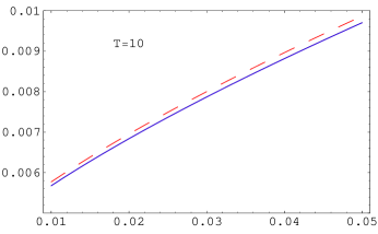
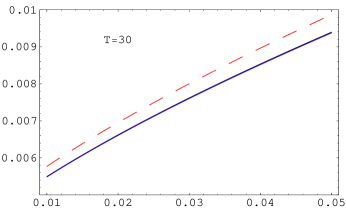
Fig. 1: The normal implied volatility $\sigma_{N}(K)-2bS_{0}$ for the shifted log-normal model comparing the exact solution (black) with the asymptotic solution $\sigma_{0}(K)$ (red dashed), and the solution including $O(T)$ corrections (solid blue). Model parameters: $S_{0}=3\%,\sigma_{0}=0.8\%,b=0.1$, and $T=10$ (left), $T=30$ (right).

The correction of $O(T)$ is $\sigma_{1}(y)$, which can be obtained from (3.1). Its power expansion around the $y=0$ point is

$$\sigma_{1}(y)=-\frac{1}{6}b^{2}\bar{\sigma}_{0}-\frac{1}{6}b^{3}y+\frac{11b^{4}}{180\bar{\sigma}_{0}}y^{2}+\cdots+\mu_{0}(\frac{b^{2}}{3\bar{\sigma}_{0}}y-\frac{b^{3}}{3\bar{\sigma}_{0}^{2}}y^{2}+O(y^{3}))$$ (67)

The ATM second order correction is obtained from (43). Neglecting the drift, its expression is

$$\sigma_{2}(0) = -\frac{1}{6}\sigma_{0}(0)H_{2}(0)=-\frac{1}{6}\sigma_{0}(y)\Big{[}3\frac{\sigma_{1}^{2}(y)}{\sigma_{0}^{2}(y)}-5\sigma_{1}(y)\sigma^{\prime\prime}_{0}(y)-\sigma_{0}(y)\sigma^{\prime\prime}_{1}(y)+(\sigma_{0}(y)\sigma^{\prime\prime}_{0}(y))^{2}\Big{]}$$ (68)

$$= -\frac{1}{6}\bar{\sigma}_{0}\Big{[}-\frac{3}{20}b^{4}\Big{]}=\frac{1}{40}\bar{\sigma}_{0}b^{4}\,.$$

Collecting all terms, the total ATM normal implied volatility in the (driftless) shifted lognormal model is given by an expansion in $b^{2}T$, whose first three terms are

$$\sigma_{N}(K=S_{0},T)=\bar{\sigma}_{0}\Big{(}1-\frac{1}{6}b^{2}T+\frac{1}{40}b^{4}T^{2}+O((b^{2}T)^{3})\Big{)}\,.$$ (69)

This can be compared with the exact solution (64), which gives for the ATM normal volatility

$$\frac{\sigma_{N}^{ATM}\sqrt{T}}{\sqrt{2\pi}}=\frac{\bar{\sigma}_{0}}{2b}[N(b\sqrt{T})-N(-b\sqrt{T})]$$ (70)

Expanding in powers of time we get

$$\sigma_{N}^{ATM}(T)=\bar{\sigma}_{0}(1-\frac{1}{6}b^{2}T+\frac{1}{40}(b^{2}T)^{2}-\frac{1}{336}(b^{2}T)^{3}+\frac{1}{3456}(b^{2}T)^{4}+O(b^{2}T)^{5})$$

The first three terms agree with the coefficients from the asymptotic expansion obtained above.

To get a sense for the numerical accuracy of the expansion, we show in Figure 1 the leading $O(T^{0})$ term $\sigma_{0}(y)$ term in the asymptotic expansion (red dashed line), together with the first subleading correction $\sigma_{0}(y)+T\sigma_{1}(y)$ (blue curve), compared with the exact solution (black curve). The agreement of the asymptotic expansion with the exact solution is very good, already at $O(T)$.

We show in Table 1 numerical results from the asymptotic expansion of the model, compared with the exact solution. The model parameters have been chosen as $\sigma_{0}=3\%,b=0.2$. The three columns show the error in the ATM normal implied volatility, with respect to the exact result. At zeroth order in the $T$ expansion, the ATM implied normal vol is $\sigma_{0}=3\%$, but at large times it deviates from this value. From Table 1, this deviation can be seen to be as large as $-0.5\%$ for $T=30$.

Table 1: Results for the ATM normal implied volatility in the shifted log-normal model, compared with the exact result, as a function of maturity $T$. The parameters of the model are $\bar{\sigma}_{0}=3\%,b=0.2$.

$T$	$b^{2}T$	$\sigma_{0}-\sigma_{\rm ex}$	$\sigma^{(1)}-\sigma_{\rm ex}$	$\sigma^{(2)}-\sigma_{\rm ex}$
1	0.04	$0.0199\%$	$-0.0001\%$	$0.0000\%$
2	0.08	$0.0395\%$	$-0.0005\%$	$0.0000\%$
5	0.2	$0.0971\%$	$-0.0029\%$	$0.0001\%$
10	0.4	$0.1885\%$	$-0.0115\%$	$0.0005\%$
20	0.8	$0.3562\%$	$-0.0438\%$	$0.0042\%$
30	1.2	$0.5058\%$	$-0.0942\%$	$0.0138\%$

Next we consider also the case with nonzero drift $\mu$. This can be included in the expressions for the coefficients of the asymptotic expansion as discussed in the previous section, see Eq. (3.1). In particular, the ATM normal implied volatility, working to order $O(T^{2})$, is given by (3.1), which for the case considered here, reads

$$\sigma_{N}(K=S_{0}+\mu T)=\bar{\sigma}_{0}+(-\frac{1}{6}b^{2}\bar{\sigma}_{0}+b\mu)T+O(T^{2})$$ (72)

where the $b\mu T$ term comes from the expansion of the leading order term $\sigma_{0}(y)$ around $y=0$.

We can check explicitly that this is reproduced by the exact solution of the model with constant drift, which is derived in the Appendix B. In Eq. (B) we obtained the first two terms of the expansion of the call price with $K=S_{0}$ in powers of the drift $\mu$.

The model (62) is related to the model in the Appendix B by a simple mapping

$$t=4b^{2}\tau$$ (73)

$$W_{t}=2b\tilde{W}_{\tau}$$ (74)

$$x_{t}=S_{\tau}+\frac{\sigma_{0}}{2b}$$ (75)

$$\mu=\frac{\mu}{4b^{2}}$$ (76)

Then if $x_{t}$ satisfies the process $dx_{t}=x_{t}dW_{t}+\mu dt$, then $S_{\tau}$ will follow the process $dS_{\tau}=(\sigma_{0}+2bS_{\tau})d\tilde{W}_{\tau}+\mu d\tau$.

In Appendix B it is shown that the price of an option with strike equal to the initial asset value $x_{0}$ is given by

$$C(K=x_{0},x_{0},t)=x_{0}\mbox{Erf}\Big{(}\frac{\sqrt{t}}{2\sqrt{2}}\Big{)}+\frac{1}{2}\mu t+O(\mu^{2})$$ (77)

The corresponding result for the model (62) is

$$C(K=S_{0},S_{0},T)=\frac{\sigma_{0}+2bS_{0}}{2b}\mbox{Erf}\Big{(}\frac{b\sqrt{T}}{\sqrt{2}}\Big{)}+\frac{1}{2}\mu T+O(\mu^{2})\,.$$ (78)

From this result we can determine the normal implied volatility in the model (62) at the point $K=S_{0}$. This can be found by comparing (78) with the Bachelier formula with $\sigma_{N}(K=S_{0},T)=\bar{\sigma}_{0}(1+c_{1}T+O(T^{2}))$, which gives $c_{1}=-\frac{1}{6}b^{2}$. This is in agreement with the result Eq. (72) for $\sigma_{1}(K=S_{0},T)$ obtained from the asymptotic expansion and confirms the absence of a term proportional to $\mu$ in $\sigma_{1}(K=S_{0},T)$.

4.2 Stochastic volatility inspired local volatility model

As a second example, we derive the short-time asymptotics of the implied normal volatility in a local volatility model inspired by a stochastic volatility model. Consider the model

$$dS(t) = \nu(t)\sigma_{D}(S(t))dW_{1}(t)$$ (79)

$$d\nu(t) = \gamma\nu(t)dW_{2}(t)\,.$$

where the two stochastic drivers have correlation $\mbox{corr }(W_{1}(t),W_{2}(t))=\rho$. The initial condition is $S(0)=F_{T},\nu(0)=1$.

We would like to use the methods of Sec. 3 to find the short time asymptotics of the normal volatility in this model. This can be done by relating first the model (79) to the SABR model [12], and then using the well-known asymptotic local volatility of the latter to find the equivalent local volatility of the model (79). We start by making the change of variable

$$z(S_{t})=\int_{F_{T}}^{S_{t}}\frac{dy}{\sigma_{D}(y)}$$ (80)

which transforms the first equation (79) into

$$dz=\nu(t)dW_{1}(t)+\mbox{ drift}$$ (81)

This is identical with the evolution of the log-price $x_{t}=\log(S_{t}/F_{t})$ in the log-normal SABR model [12], so we can take over the asymptotic solution of the SABR model for the short-time asymptotic limit [12, 13]. The following one-dimensional process has the same terminal distribution of $x(t)$ as the two-dimensional stochastic volatility model at leading order in a short-time expansion [13, 14]

$$\sigma_{\rm eff}^{2}(z)=\gamma^{2}z^{2}-2\rho\gamma z+1\,.$$ (82)

Higher order terms in the asymptotic expansion of the SABR model have been obtained in [16, 17, 18, 19].

The process for $z_{t}$ can be converted into a process for the original asset price $S(t)$ by an application of the Ito lemma

$$dS(t)=\sigma_{D}(S(t))\sigma_{\rm eff}(z(S(t))dW(t)$$ (83)

where the function $z(S)$ is given in (80).

We can use now the short-time asymptotics (27) applied to this one-dimensional model to derive the leading asymptotics for the normal smile in the stochastic volatility model (79)

$$\sigma_{N,0}(K,T) = \frac{K-F_{T}}{\int_{F_{T}}^{K}\frac{dS}{\sigma_{D}(S)\sigma_{\rm eff}(z(S))}}=\frac{K-F_{T}}{\int_{0}^{z(K)}\frac{dx}{\sigma_{\rm eff}(x)}}=\gamma\frac{K-F_{T}}{D(\gamma z(K))}$$ (84)

where

$$D(x)=\log\frac{\sqrt{1-2\rho x+x^{2}}+x-\rho}{1-\rho}$$ (85)

and

$$z(K)=\int_{F_{T}}^{K}\frac{dy}{\sigma_{D}(y)}\,.$$ (86)

The result (84) gives the short-time asymptotics for the normal implied volatility of the stochastic volatility model (79).

We consider in the following the case of the normal SABR model with constant local volatility $\sigma_{D}(S)=\sigma_{0}$, and study the normal implied volatility of the local volatility model (83). The argument of the local volatility depends on the variable $z(S(t),S(0))=1/\sigma_{0}(S(t)-S(0))$, such that we obtain the local volatility model

$$dS(t)=\sqrt{\sigma_{0}^{2}-2\rho\gamma\sigma_{0}y+\gamma^{2}y^{2}}dW(t)$$ (87)

with $y=S(t)-S(0)$. Although the original stochastic volatility model (79) is well-defined only for non-positive correlation $\rho\leq 0$ [15], we will use the local volatility (83) for both positive and negative values of $\rho$, effectively ignoring its origin as a stochastic volatility model.

One can use now the results of Section 2 to derive the normal implied volatility of this model as an expansion in $T$. The leading order result is given in Eq. (84), and the first subleading correction in Eq. (3.1).

We show in Figure 2 the results for the normal implied volatility in the model (87) at leading order in $T$, and including the $O(T)$ correction $\sigma_{1}(y)$. These are compared with an exact numerical solution. We note that for moderate maturities the agreement obtained by keeping only the first subleading term is satisfactory.

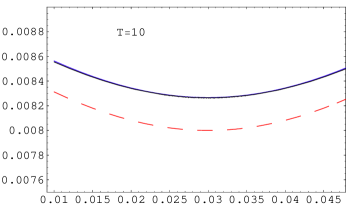
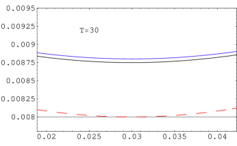
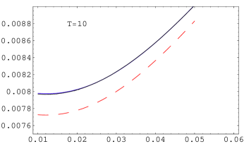
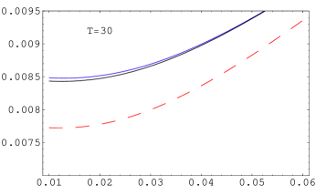
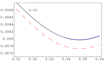
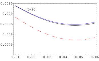
Fig. 2: The asymptotic expansion for the normal implied volatility of the SABR-like model (87) compared with the exact numerical solution (black curves) for two maturities: $T=10$ (left), and $T=30$ (right). The red dashed curves show the asymptotic solution $\sigma_{0}(K)$, and the blue curve shows the asymptotic solution including the $O(T)$ correction. Model parameters: $S_{0}=3\%,\sigma_{0}=0.8\%,\gamma=0.2$. The correlation is $\rho=0\%$ (upper plots), $\rho=30\%$ (middle plots) and $\rho=-30\%$ (lower plots).

5 Nonanalytic local volatility

The asymptotic expansion for the normal implied volatility in powers of $T$ presented in Sections 2 and 3 is applicable only for analytic local volatility functions $\sigma_{D}(S)$. If $\sigma_{D}(S)$ is not analytic, the asymptotic expansion fails, and new terms which are non-analytic in time can appear.

To illustrate this phenomenon, consider a model with local volatility which has a discontinuous derivative

$$\sigma_{D}(y)=\left\{\begin{array}[]{cc}\sigma_{0}+2b_{L}y\,,&y<0\\ \sigma_{0}+2b_{R}y\,,&y>0\\ \end{array}\right.$$ (90)

.

According to the asymptotic expansion formula, the implied volatility $\sigma_{0}(y)$ (and all higher order terms) depends only on the values of the local volatility in the interval $(S_{0},K)$, but not on its values outside this interval. For this case, it implies that the implied volatility $\sigma_{N}(y)$ for $y>0(y<0)$ should depend only on $b_{R}(b_{L})$. We show in Fig. 3 the exact solution for the implied volatility $\sigma_{N}(y)$, obtained using a numerical solution in Mathematica (solid lines), and the leading asymptotic results $\sigma_{0}(K)$, from the BBF formula (dashed lines). The three curves correspond to $b_{L}=-0.1$ (red), $b_{L}=0$ (blue), and $b_{L}=0.1$ (black), keeping $b_{R}=0.1$ fixed. We observe that the implied volatility for $y>0$ depends strongly on the value of $b_{L}$, which determines the local volatility outside the region $(S_{0},K)$. Although for $b_{L}=0.1$ the exact result is in good agreement with the asymptotic expansion, the agreement becomes far worse for $b_{L}=0,-0.1$.

In order to understand better the poor convergence of the asymptotic expansion in the case $b_{L}\neq b_{R}$, we consider in more detail the particular case of the model (90) with $-b_{L}=b_{R}\equiv b$, for which an exact solution is known [23]. The exact solution for the ATM implied volatility can be written as a sum of two terms (see the Appendix for a detailed proof). The first term coincides with the solution of the shifted log-normal model considered above with $b=b_{R}$, and the second term gives the correction due to the discontinuity at $y<0$

$$\sigma(0,t)=\sigma_{1}(0,t)+\sigma_{2}(0,t)$$ (91)

with

$$\sigma_{1}(0,t) = \sigma_{0}\sqrt{\frac{\pi}{2}}\frac{1}{b\sqrt{t}}\mbox{Erf}(\frac{b\sqrt{t}}{\sqrt{2}})$$ (92)

$$\sigma_{2}(0,t) = \frac{1}{2}\sigma_{0}e^{-\frac{1}{2}b^{2}t}+\frac{1}{2}\sigma_{0}\sqrt{\frac{\pi}{2}}\Big{[}b\sqrt{t}+b\sqrt{t}\mbox{Erf}(\frac{b\sqrt{t}}{\sqrt{2}})-\frac{1}{b\sqrt{t}}\mbox{Erf}(\frac{b\sqrt{t}}{\sqrt{2}})\Big{]}$$ (93)

Expanding the exact implied volatility in powers of time, the first term $\sigma_{1}(0,t)$ reproduces the result of the shifted log-normal model (4.1) corresponding to the local volatility in the $y>0$ extrapolated to the entire region $\sigma_{D}(y)=\sigma_{0}+2by$

$$\sigma_{1}(0,t) = \sigma_{0}(1-\frac{1}{6}b^{2}t+\frac{1}{40}b^{4}t^{2}-\frac{1}{336}b^{6}t^{3}+\cdots)$$ (94)

However, there is a second correction $\sigma_{2}(0,t)$, which has the time expansion

$$\sigma_{2}(0,t) = \sigma_{0}(\frac{1}{2}\sqrt{\frac{\pi}{2}}b\sqrt{t}+\frac{1}{3}b^{2}t-\frac{1}{30}b^{4}t^{2}+\frac{1}{280}b^{6}t^{3}+\cdots)$$ (95)

The term $\sigma_{2}(0,t)$ is not reproduced by the asymptotic expansion discussed in Section 3. Even more surprising, it contains a term of $O(\sqrt{t})$, which is not allowed by the asymptotic expansion of the Dupire equation in volatility form. This term largely accounts for the large deviation from the asymptotic result in Figure 3. The absence of the term $\sigma_{2}(0,t)$ and its nonanalytic dependence on time signal a failure of the asymptotic expansion for the model (90).

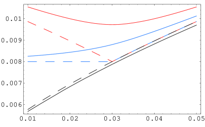
Fig. 3: The normal implied volatility $\sigma_{N}(K)$ for the model (90) with parameters $S=3\%,\sigma_{0}=0.8\%,b_{L}=0.1\mbox{(black}),0\mbox{(blue)},-0.1\mbox{(red)},b_{R}=0.1$ and $T=10$. The solid lines show exact numerical solutions of the Dupire equation, while the dashed lines correspond to the asymptotic solution $\sigma_{0}(K)$.

This failure appears to be generic for nonanalytic local volatility functions. We prove next the following result: in any local volatility model with a local volatility function which has a jump in the derivative at the forward point

$$\Delta(\sigma^{2}_{D}(F_{T}))^{\prime}=\partial_{K}\sigma^{2}_{D}(K=F_{T}+\varepsilon)-\partial_{K}\sigma^{2}_{D}(K=F_{T}-\varepsilon)$$ (96)

the time expansion of the ATM normal implied volatility contains a term $\sim\sqrt{T}$ which is nonanalytic in time, and which is proportional to the jump of the derivative

$$\sigma_{N}(F_{T},T)=\sigma_{D}(F_{T})+\frac{1}{16}\sqrt{\frac{\pi}{2}}\sigma_{D}(F_{T})\sqrt{T}\Delta(\sigma^{2}_{D}(F_{T}))^{\prime}+O(T)$$ (97)

This anomalous term reproduces the $O(\sqrt{T})$ term in Eq. (95) for the model (90), for which the jump of the derivative is $\Delta\sigma^{\prime}_{D}(F_{T})=4b$.

The proof of this result makes use of perturbation theory for linear operators [24, 25]. We would like to solve the Dupire equation (9) which we repeat here for convenience. This gives the price of a call option $C(K,T)$ at time $T$, and reads

$$\partial_{T}C(K,T)=\frac{1}{2}\sigma_{D}^{2}(K)\partial_{K}^{2}C(K,T)$$ (98)

with the initial condition $C(K,0)=\mbox{max}(K-S_{0},0)$. For simplicity, we assumed a zero drift term $\mu_{T}=0$, and assumed the local volatility to be time-homogeneous. This equation is identical with the heat equation with position dependent conductivity $\sigma_{D}(K)$, and the initial condition $C(K,0)=\mbox{max}(K-S_{0},0)$.

The solution can be written formally in operator form as

$$C(K,T)=\exp\Big{(}\hat{L}(K)T\Big{)}C(K,0)=\exp\Big{(}\hat{L}_{0}T+(\hat{L}-\hat{L}_{0})T\Big{)}C(K,0)$$ (99)

where we denoted the differential operators

$$\hat{L}_{0}(K) = \frac{1}{2}\sigma_{D}^{2}(S_{0})\partial_{K}^{2}$$ (100)

$$\hat{L}(K) = \frac{1}{2}\sigma_{D}^{2}(K)\partial_{K}^{2}$$ (101)

The solution with $\hat{L}=\hat{L}_{0}$ is well-known, and can be written as a convolution of the initial condition with the heat kernel

$$G_{0}(x,t;y,0)=\frac{1}{\sqrt{2\pi t}}\exp(-\frac{(x-y)^{2}}{2t})$$ (102)

The solution of the unperturbed equation $\partial_{T}C_{0}(K,T)=\hat{L}_{0}(K)C(K,T)$ is given by the convolution

$$C_{0}(K,T)=\int_{-\infty}^{\infty}dyG_{0}(y,\sigma_{0}^{2}T;y,0)\mbox{max}(y-S_{0},0)$$ (103)

where we denoted for simplicity $\sigma_{D}(S_{0})=\sigma_{0}$. The integral can be computed in closed form, and the result is the well-known Bachelier formula (8).

We will treat the difference $\Delta\hat{L}\equiv\hat{L}-\hat{L}_{0}$ as a perturbation, and write the solution (99) as an expansion in powers of $\Delta\hat{L}$

$$C(K,T)=C_{0}(K,T)+C_{1}(K,T)+C_{2}(K,T)+\cdots$$ (104)

The term of zeroth order $C_{0}(K,T)$ is identical to the Bachelier result. The term of first order in the perturbation is given by a triple integral

$$C_{1}(K,T)=\int_{-\infty}^{\infty}dy\int_{-\infty}^{\infty}du\int_{0}^{T}d\tau G_{0}(K,\sigma_{0}^{2}T;u,\sigma_{0}^{2}\tau)\Delta\hat{L}(u)G_{0}(u,\sigma_{0}^{2}\tau;y,0)\mbox{max}(y-S_{0},0)$$

The action of the operator $\Delta\hat{L}(u)$ can be expressed as

$$\Delta\hat{L}(u)G_{0}(u,\sigma_{0}^{2}\tau;y,0) = \frac{\sigma_{D}^{2}(u)-\sigma_{0}^{2}}{\sigma_{0}^{2}}\partial_{\tau}G_{0}(u,\sigma_{0}^{2}\tau;y,0)$$

$$=\frac{\sigma_{D}^{2}(u)-\sigma_{0}^{2}}{\sigma_{0}^{2}}\Big{(}-\frac{1}{2\tau}+\frac{(u-y)^{2}}{2\sigma_{0}^{2}\tau^{2}}\Big{)}G_{0}(u,\sigma_{0}^{2}\tau;y,0)\,.$$

Let us examine in some detail the dependence on time $T$ of the first order perturbation $C_{1}(K,T)$ for the ATM case $K=S_{0}$. For simplicity, shift the origin of the $y$ axis such that $S_{0}=0$. It is also useful to introduce rescaled variables

$$\bar{y}=\frac{y}{\sigma_{0}\sqrt{T}}\,,\qquad\bar{u}=\frac{u}{\sigma_{0}\sqrt{T}}\,,\qquad\lambda=\frac{\tau}{T}\,.$$ (107)

in terms of which the heat kernel is expressed as

$$G_{0}(0,\sigma_{0}^{2}T;u,\sigma_{0}^{2}\tau)=\frac{1}{\sigma_{0}\sqrt{T}}G_{0}(0,1;\bar{u},\lambda)$$ (108)

We have in terms of these variables

$$C_{1}(0,T) = \sigma_{0}\sqrt{T}\int_{-\infty}^{\infty}d\bar{y}d\bar{u}\int_{0}^{1}d\lambda G_{0}(0,1;\bar{u},\lambda)\frac{\sigma_{D}^{2}(\bar{u}\sigma_{0}\sqrt{T})-\sigma_{0}^{2}}{\sigma_{0}^{2}}$$

$$\times\Big{(}-\frac{1}{2\lambda}+\frac{(\bar{u}-\bar{y})^{2}}{2\lambda^{2}}\Big{)}G_{0}(\bar{u},\lambda;\bar{y},0)(\bar{y})_{+}$$

A similar rescaling gives for the zeroth order term

$$C_{0}(0,T)=\sigma_{0}\sqrt{T}\int_{-\infty}^{\infty}d\bar{y}G_{0}(\bar{u},\lambda;\bar{y},0)(\bar{y})_{+}$$ (110)

We observe that the overall scaling factor $\sqrt{T}$ is the same for $C_{0}$ and $C_{1}$, and the only new time dependence in $C_{1}$ appears from the factor involving the local volatility $\sigma_{D}^{2}(\bar{u}\sigma_{0}\sqrt{T})$. Assuming analyticity, Taylor expansion of this factor produces both integer and half-integer powers of time

$$\sigma_{D}^{2}(\bar{u}\sigma_{0}\sqrt{T})-\sigma_{0}^{2}=\sigma_{0}\sqrt{T}\bar{u}(\sigma_{D}^{2}(0))^{\prime}+\frac{1}{2}(\sigma_{0}\sqrt{T})^{2}\bar{u}^{2}(\sigma_{D}^{2}(0))^{\prime\prime}+\cdots$$ (111)

Table 2: Contributions to the ATM implied volatility from the $n$-th order of perturbation in $\Delta\hat{L}$.

$n$	ATM implied vol
1	$T^{\frac{1}{2}},T,T^{\frac{3}{2}},T^{2},\cdots$
2	$T,T^{\frac{3}{2}},T^{2},\cdots$
3	$T^{\frac{3}{2}},T^{2},\cdots$
4	$T^{2},\cdots$

At this point we stop and examine the structure of the time-dependent terms at higher orders in perturbation theory. The $n$-th order in perturbation theory $C_{n}(K,T)$ will be given by a $2n+1$-dimensional integral, which includes $n$ double integrals over intermediate space-time variables, plus one final integral over the initial condition. The time dependence will consist of an overall $\sigma_{0}\sqrt{T}$ factor as in $C_{0,1}(K,T)$ plus terms arising from the presence of $n$ factors of the form (111). The resulting contributions at each order $n$ in perturbation theory can be easily obtained and are shown in Table 2.

It is clear that only the first order in perturbation theory can contribute a term of $O(\sqrt{T})$ to the ATM implied volatility. However, upon computing the integrals over $\bar{u},\bar{y}$ we get a vanishing result

$$\int_{0}^{\infty}d\bar{y}\bar{y}\int_{-\infty}^{\infty}d\bar{u}G_{0}(0,1;\bar{u},\lambda)\bar{u}(-\frac{1}{2\lambda}+\frac{(\bar{u}-\bar{y})^{2}}{2\lambda^{2}})G_{0}(\bar{u},\lambda;\bar{y},0)=\int_{0}^{\infty}d\bar{y}\bar{y}^{2}e^{-\frac{1}{2}\bar{y}^{2}}(3-\bar{y}^{2})=0\,.$$

This proves the absence of a $O(\sqrt{T})$ term in the ATM implied volatility for the case of an analytical local volatility. This is in agreement with the results of Sections 2, 3, which considered only this case.

However, the situation is very different if we assume a nonanalytical local volatility. Taking an expansion for $\sigma_{D}^{2}(\bar{u}\sigma_{0}\sqrt{T})$ with a linear term of the form

$$\sigma_{D}^{2}(\bar{u}\sigma_{0}\sqrt{T})-\sigma_{0}^{2}=\left\{\begin{array}[]{cc}\bar{u}\sigma_{0}\sqrt{T}b_{R}&\mbox{if }\bar{u}>0\\ \bar{u}\sigma_{0}\sqrt{T}b_{L}&\mbox{if }\bar{u}\leq 0\\ \end{array}\right.$$ (115)

the integration over $\bar{u},\bar{y}$ does not vanish anymore, and the result is proportional with the discontinuity of the derivative $b_{R}-b_{L}$

$$C_{1}(0,T)=\sigma_{0}\sqrt{T}\Big{(}\frac{1}{32}\sigma_{0}\sqrt{T}(b_{R}-b_{L})\Big{)}$$ (116)

Using the relation $C(0,T)=\frac{1}{\sqrt{2\pi}}\sigma_{N}(0,T)\sqrt{T}$, we obtain from this result the $O(\sqrt{T})$ term in the ATM implied volatility. This concludes the proof of the relation (97).

The explicit result for the normal implied volatility Eq. (95) for the model (90) contains only one non-analytic term $\sim\sqrt{T}$, but not other terms of similar form, e.g. $T^{3/2},T^{5/2},\cdots$. It would be interesting to investigate whether this is a general result, or if it holds only in the specific model (90).

Although the relation (97) was proved for the ATM normal volatility, a similar result holds also for the ATM log-normal volatility. This is related to the former by the exact relation (120)

$$\sigma_{N}(0,T)=F_{T}\sqrt{\frac{2\pi}{T}}\mbox{Erf}\Big{(}\frac{\sigma_{BS}(0,T)\sqrt{T}}{2\sqrt{2}}\Big{)}$$ (117)

In the short-maturity limit $T\to 0$ this reduces to the well-known relation $\sigma_{N}(0)=F_{T}\sigma_{BS}(0)$. The relation between $\sigma_{N}(0,T)$ and $\sigma_{BS}(0,T)$ is an analytical function of time, which implies that a term proportional to $\sqrt{T}$ in the expansion of the ATM normal implied volatility will introduce such a contribution also in the ATM log-normal implied volatility.

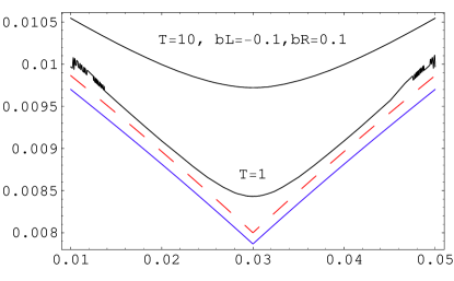
Fig. 4: The normal implied volatility $\sigma_{N}(K)$ for the model (90) comparing the exact solution (black) with the asymptotic solution $\sigma_{0}(K)$ (red dashed), and the solution including $O(T)$ corrections (solid blue). Model parameters: $S=3\%,\sigma_{0}=0.8\%,T=10$. $b_{L,R}$ are as shown in the plots.

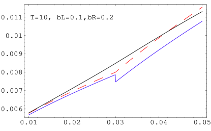
Fig. 5: Discontinuity of the asymptotic solution at $O(T)$ for the model (90), with $|b_{L}|\neq|b_{R}|$. As explained in text, the subleading correction $\sigma_{1}(y)$ is discontinuous at $y=0$. The black curve shows the exact (numerical) solution, the red dashed curve shows the asymptotic solution $\sigma_{0}(K)$, and the blue curve shows the asymptotic solution including $O(T)$ corrections. Model parameters: $S=3\%,\sigma_{0}=0.8\%,T=10,b_{L}=0.1,b_{R}=0.2$.

Another manifestation of the failure of the asymptotic expansion for non-analytic local volatility functions is the prediction of a discontinuity in the implied volatility. This can happen for example in the model (90) at order $O(T)$ in the $T$ expansion, provided that $|b_{L}|\neq|b_{R}|$. The correction of $O(T)$ to the normal implied volatility is given by Eq. (3.1). The jump of the subleading correction can be obtained from the power series expansion of $\sigma_{1}(y)$ in the shifted log-normal model, and is

$$\sigma_{1}(0+\epsilon)-\sigma_{1}(0-\epsilon)=-\frac{1}{6}(b_{R}^{2}-b_{L}^{2})\sigma_{0}$$ (118)

This discontinuity is shown in Figure 3 for a specific choice of the model parameters. Such a discontinuity is clearly an artifact of the naive application of the asymptotic expansion, as the numerical solution is continuous everywhere.

6 Conclusions

In this paper we extended the short time asymptotic expansion method to local volatility models described in terms of normal volatility, as opposed to log-normal volatility. A description in terms of normal implied volatility appears naturally in the context of interest rates, which can become negative in regimes of small interest rates. The Dupire equation can be formulated as a nonlinear equation for the implied normal volatility, which can be solved by an asymptotic expansion in powers of time $T$. This equation is similar (although in a different independent variable - the difference strike $y=K-F_{T}$ as opposed to the log-strike $x=\log(K/F_{T})$) to the usual BBF equation [5], from which it differs only at $O(T^{2})$.

We present explicit solutions for the coefficients of the $O(T),O(T^{2})$ terms in the small-time expansion of the normal implied volatility. The drift term in the $O(T)$ coefficient can be expressed as a simple integral over the zeroth order coefficient and the local volatility. We point out that the drift contribution vanishes at the ATM point $K=S_{0}$ in the $O(T)$ term. This absence is verified on the explicit example of the shifted log-normal model with constant drift, for which an exact solution can be obtained.

We studied the convergence of the asymptotic expansion on two examples of analytical local volatility: shifted log-normal model with and without drift, and a model inspired from stochastic volatility models for which the local volatility is the square root of a quadratic polynomial of strike. We found generally good agreement, even when keeping only the first two terms $O(1),O(T)$ in the small-time expansion.

The asymptotic expansion of the implied volatility in integer powers of $T$ can fail if the local volatility is a nonanalytic function. Using perturbation theory techniques, we show that in local volatility models where the local volatility has a discontinuous derivative at the ATM point, the ATM normal implied volatility contains nonanalytic dependence on time, proportional to $\sqrt{T}$. Furthermore, the coefficient of this term is simply determined, and is proportional to the jump of the derivative at the nonanalyticity point. Although these results have been proven for the normal implied volatility, similar results must hold also for the log-normal implied volatility, which is related to the former by an analytical function of time.

Another manifestation of the failure of the usual asymptotic expansion for such models is the presence of a jump discontinuity in the $O(T)$ contribution to the implied volatility. These observations show that the usual asymptotic expansion can fail for non-analytic local volatility functions, and has to be used with care in such situations.

Appendix A Relation between the normal and log-normal implied volatilities

We quote here an exact relation between normal and log-normal implied volatilities valid for arbitrary maturity $T$, but for small deviations from the ATM point $y=K-F_{T}\ll F_{T}$. This takes the form of an expansion in $y/F_{T}$, and the first few terms are

$$w_{N}(y,T) = F_{T}\left\{\sqrt{2\pi}\mbox{Erf}\Big{(}\frac{w}{2\sqrt{2}}\Big{)}+\sqrt{\frac{\pi}{2}}\mbox{Erf}\Big{(}\frac{w}{2\sqrt{2}}\Big{)}\frac{y}{F_{T}}\right.$$

$$+ \left.\Big{(}\frac{1}{2w}e^{-w^{2}/8}-\frac{1}{2\sqrt{2\pi}\mbox{Erf}\Big{(}\frac{w}{2\sqrt{2}}\Big{)}}\Big{)}\Big{(}\frac{y}{F_{T}}\Big{)}^{2}+O\Big{(}\frac{y}{F_{T}}\Big{)}^{3}\right\}$$

We denoted here $w_{N}(y,T)=\sigma_{N}\sqrt{T}$ and $w(y,T)=\sigma_{BS}\sqrt{T}$ the square roots of the normal and log-normal variances, respectively.

The ATM implied volatilities satisfy the relation

$$\sigma_{N}(0,T)=F_{T}\sqrt{\frac{2\pi}{T}}\mbox{Erf}\Big{(}\frac{\sigma_{BS}(0,T)\sqrt{T}}{2\sqrt{2}}\Big{)}$$ (120)

which reduces in the short-maturity limit $T\to 0$ to the well-known relation $\sigma_{N}(0)=F_{T}\sigma_{BS}(0)$.

Taking the derivative with respect to strike at the ATM point gives an exact relation between the normal and log-normal skews

$$\sigma^{\prime}_{N}(0,T)=F_{T}[\sigma^{\prime}_{BS}(0,T)+\sqrt{\frac{\pi}{2}}\frac{1}{\sqrt{T}}\mbox{Erf}\Big{(}\frac{\sigma_{BS}(0,T)\sqrt{T}}{2\sqrt{2}}\Big{)}]$$ (121)

which reduces in the short time limit to

$$\sigma^{\prime}_{N}(F_{T}) = \frac{1}{2}\sigma_{BS}(F_{T})+F_{T}\sigma^{\prime}_{BS}(F_{T})$$ (122)

The asymptotic results of Sec. 2 give an exact relation between the normal and log-normal implied volatilities, valid in the short-time asymptotic limit. We limit ourselves to the case of time-homogeneous local volatility. The relations (28) and (27) express both of them in terms of the same local volatility $\sigma_{D}(x)$. Eliminating the local volatility gives a direct relation between the two types of implied volatilities.

The starting point is Eq. (27), where we substitute the local volatility $\sigma_{D}(y)$ with its expression in terms of the log-normal volatility

$$\sigma_{D}(x)=\frac{\sigma_{BS}(x)}{1-\frac{x}{\sigma_{BS}(x)}\partial_{x}\sigma_{BS}(x)}$$ (123)

with $x=\log(K/F_{T})$.

The integral in the denominator of (27) can be performed by integration by parts

$$\int_{F_{T}}^{K}dL\frac{1}{\sigma_{D}(L)}=\int_{0}^{x}\frac{dy}{\sigma_{BS}(y)}-\int_{0}^{x}\frac{y}{\sigma^{2}_{BS}(y)}d\sigma_{BS}=\frac{x}{\sigma_{BS}(x)}$$ (124)

and we find the very simple result

$$\sigma_{N}(K)=\sigma_{BS}(K)\frac{K-F_{T}}{\log\frac{K}{F_{T}}}$$ (125)

Expanding around this point one can find relations among the skews and curvatures (convexities) of the normal and log-normal ATM skews, valid in the short time limit. We quote here the relation among convexities

$$\sigma^{\prime\prime}_{N}(F_{T}) = -\frac{1}{6F_{T}}\sigma_{BS}(F_{T})+\sigma^{\prime}_{BS}(F_{T})+F_{T}\sigma^{\prime\prime}_{BS}(F_{T})$$ (126)

Appendix B Log-normal process with constant drift

As an explicit example of local volatility model of the type (4) with non-zero drift, we consider the simplest such process, with log-normal volatility and constant drift

$$dx_{t}=x_{t}dW_{t}+\mu dt$$ (127)

We will compute the normal implied volatility in this model, and compare its small time expansion with the asymptotic expansion derived in Sec. 3. As noted in Sec. 4, this explicit example confirms the correctness of the $O(T)$ correction to the normal implied volatility (3.1).

The stochastic differential equation (127) can be integrated in closed form with the result

$$x_{t}=x_{0}\exp(W_{t}-\frac{1}{2}t)+\mu\int_{0}^{t}ds\exp(W_{t}-W_{s}-\frac{1}{2}(t-s))\,.$$ (128)

From this expression it is clear that $x_{t}$ is restricted to the range $x_{t}>0$, provided that $\mu\geq 0$. In the following we will restrict ourselves to the case $\mu\geq 0$.

The mean and variance of $x_{t}$ are

$$E[x_{t}]=x_{0}+\mu t\,,$$

$$\mbox{var}(x_{t})=E[x_{t}^{2}]-E[x_{t}]^{2}=x_{0}^{2}(e^{t}-1)+2x_{0}\mu(e^{t}-1-t)+2\mu^{2}(e^{t}-1-t-\frac{t^{2}}{2})\,.$$

The process for $z_{t}=\log(x_{t})$ is mean-reverting around $z_{\rm mid}=\log(2\mu)$. This reads $dz_{t}=dW_{t}+(\mu e^{-z_{t}}-\frac{1}{2})dt$, which is similar to the Ornstein-Uhlenbeck process, but with an exponential mean-reverting term. From Eq. (B) we see that the variance of $x_{t}$ increases with $t$ and is unbounded, which is different from the OU proces, for which it approaches a finite limit as $t\to\infty$.

We would like to compute the price of a call option on $x_{t}$ with strike $K$ conditional on $x_{0}$ at $t=0$

$$C(K,t)=E[(x_{t}-K)_{+}|x_{0},t=0]$$ (130)

It satisfies the Dupire equation

$$\partial_{t}C(K,t)=\frac{1}{2}K^{2}\partial_{K}^{2}C(K,t)-\mu\partial_{K}C(K,t)$$ (131)

with the boundary conditions

$$C(K,0)=(x_{0}-K)_{+}$$ (132)

$$C(0,t)=x_{0}+\mu t\,,\qquad\partial_{K}C(K,t)|_{K=0}=-1\,,\qquad\lim_{K\to\infty}\partial_{K}C(K,t)=0\,.$$ (133)

We will solve the Dupire equation (131) using Laplace transform methods. Define the Laplace transform of the call price with respect to time

$$y(x,s)=\int_{0}^{\infty}dte^{-st}C(x,t)$$ (134)

This satisfies the Dupire equation in Laplace transformed form

$$\frac{1}{2}x^{2}y^{\prime\prime}(x)-\mu y^{\prime}(x)-sy(x) = x-x_{0}\,,\qquad 0\leq x\leq x_{0}$$

$$= 0\,,\qquad\qquad\quad x>x_{0}$$

with boundary conditions

$$y(0,s)=\frac{x_{0}}{s}+\frac{\mu}{s^{2}}\,,\qquad y^{\prime}(0,s)=-\frac{1}{s}\,,\qquad\lim_{x\to\infty}y^{\prime}(x,s)=0\,.$$ (136)

The solution of (B) is given by the sum of a particular solution of the inhomogeneous equation plus the most general solution of the homogeneous equation

$$y(x) = \left\{\begin{array}[]{cc}-\frac{1}{s}(x-x_{0}-\frac{\mu}{s})+c_{1}f_{1}(x)+c_{2}f_{2}(x)&x<x_{0}\\ d_{2}f_{2}(x)&x>x_{0}\\ \end{array}\right.$$ (139)

where $f_{1,2}(x)$ are the solutions of the homogeneous equation. They are

$$f_{1}(x) = x^{\lambda_{1}}{}_{1}F_{1}(-\lambda_{1},2\lambda_{2};-\frac{2\mu}{x})$$ (140)

$$f_{2}(x) = x^{\lambda_{2}}{}_{1}F_{1}(-\lambda_{2},2\lambda_{1};-\frac{2\mu}{x})$$ (141)

with ${}_{1}F_{1}(a,b,z)$ the confluent hypergeometric function, and $\lambda_{1,2}$ are functions of $s$

$$\lambda_{1}=\frac{1}{2}(1+\sqrt{1+8s})>0\,,\qquad\lambda_{2}=\frac{1}{2}(1-\sqrt{1+8s})<0$$ (142)

In the $x>x_{0}$ region we kept only the second solution $f_{2}(x)$ since it is the only one which satisfies the condition $y^{\prime}(x)\to 0$ as $x\to\infty$. For large values of the argument $x$ the asymptotics of the solutions is

$$f_{1}(x)\simeq x^{\lambda_{1}}\,,\qquad f_{2}(x)\simeq x^{\lambda_{2}}$$ (143)

such that $f_{1}(x)$ is increasing while $f_{2}(x)$ decreases approaching 0 as $x\to\infty$.

The wronskian of the two solutions of the homogeneous equation $f_{1,2}(x)$ is

$$f_{1}(x)f^{\prime}_{2}(x)-f^{\prime}_{1}(x)f_{2}(x)=(\lambda_{2}-\lambda_{1})\exp(-\frac{2\mu}{x})=-\sqrt{1+8s}\exp(-\frac{2\mu}{x})\,.$$ (144)

The boundary conditions at $x=0$ (136) require that the constants $c_{1,2}$ satisfy the conditions

$$c_{1}f_{1}(0)+c_{2}f_{2}(0)=0$$ (145)

$$c_{1}f^{\prime}_{1}(0)+c_{2}f^{\prime}_{2}(0)=0\,.$$ (146)

This will have nonzero solutions for $c_{1,2}$ only if the wronskian of the two functions vanishes at $x=0$. Using the explicit expression in (144) this is seen to be indeed the case. Only one of the two equations above is independent; we will choose the first one.

The limit of the functions $f_{1,2}(x)$ at $x=0$ is

$$f_{1}(0)=(2\mu)^{\lambda_{1}}\frac{\Gamma(2\lambda_{2})}{\lambda_{2}\Gamma(\lambda_{2})}\,,\qquad f_{2}(0)=(2\mu)^{\lambda_{2}}\frac{\Gamma(2\lambda_{1})}{\lambda_{1}\Gamma(\lambda_{1})}$$ (147)

Another condition on the constants $c_{1,2},d_{2}$ follows from requiring continuity of $y(x)$ at $x=x_{0}$

$$c_{1}f_{1}(x_{0})+c_{2}f_{2}(x_{0})-d_{2}f_{2}(x_{0})=-\frac{\mu}{s^{2}}$$ (148)

Finally, another condition is obtained from the normalization of the integrated pdf

$$\int_{0}^{\infty}dxy^{\prime\prime}(x)=\int_{0}^{x_{0}}dx(c_{1}f^{\prime\prime}_{1}(x)+c_{2}f^{\prime\prime}_{2}(x))+\int_{x_{0}}^{\infty}dxd_{2}f^{\prime\prime}_{2}(x)=\frac{1}{s}$$ (149)

which gives

$$c_{1}f^{\prime}_{1}(x_{0})+c_{2}f^{\prime}_{2}(x_{0})-d_{2}f^{\prime}_{2}(x_{0})=\frac{1}{s}$$ (150)

Together with (145) and (148) this equation fixes the constants $c_{1,2},d_{2}$. These constants are found by solving the equations

$$c_{1}f_{1}(0)+c_{2}f_{2}(0)=0$$ (151)

$$c_{1}f_{1}(x_{0})+c_{2}f_{2}(x_{0})-d_{2}f_{2}(x_{0})=-\frac{\mu}{s^{2}}$$ (152)

$$c_{1}f^{\prime}_{1}(x_{0})+c_{2}f^{\prime}_{2}(x_{0})-d_{2}f^{\prime}_{2}(x_{0})=\frac{1}{s}$$ (153)

The solution is

$$c_{1} = \frac{f_{2}(x_{0})+(\mu/s)f^{\prime}_{2}(x_{0})}{(f^{\prime}_{1}(x_{0})f_{2}(x_{0})-f_{1}(x_{0})f^{\prime}_{2}(x_{0}))s}=\frac{f_{2}(x_{0})+(\mu/s)f^{\prime}_{2}(x_{0})}{s\sqrt{1+8s}}\exp(\frac{2\mu}{x_{0}})$$ (154)

$$c_{2} = -\frac{f_{1}(0)[f_{2}(x_{0})+(\mu/s)f^{\prime}_{2}(x_{0})]}{f_{2}(0)(f^{\prime}_{1}(x_{0})f_{2}(x_{0})-f_{1}(x_{0})f^{\prime}_{2}(x_{0}))s}$$

$$= (2\mu)^{\sqrt{1+8s}}\frac{\lambda_{1}\Gamma(\lambda_{1})\Gamma(2\lambda_{2})}{\lambda_{2}\Gamma(\lambda_{2})\Gamma(2\lambda_{1})}\frac{[f_{2}(x_{0})+(\mu/s)f^{\prime}_{2}(x_{0})]}{s\sqrt{1+8s}}\exp(\frac{2\mu}{x_{0}})$$

$$d_{2} = \frac{f_{1}(0)f_{2}(x_{0})-f_{1}(x_{0})f_{2}(0)+[f_{1}(0)f^{\prime}_{2}(x_{0})-f^{\prime}_{1}(x_{0})f_{2}(0)](\mu/s)}{f_{2}(0)(f_{1}(x_{0})f^{\prime}_{2}(x_{0})-f^{\prime}_{1}(x_{0})f_{2}(x_{0}))s}\,.$$ (156)

This completes the solution of the Laplace transformed Dupire equation (B). The call price $C(K,t)$ is obtained by taking the inverse Laplace transform of the solution $y(x,s)$ given in Eq. (139) with the coefficients $c_{1,2},d_{2}$ given in (154), (B), (156).

We consider next the explicit result for $y(x_{0},s)$, which is the Laplace transform over time of the “ATM” call price (the quotation marks are a reminder that this is the ATM point only for the case of zero drift; in the presence of the drift the ATM point corresponds to $x=x_{0}+\mu/s$)

$$y(x_{0},s) = \frac{\mu}{s^{2}}+\frac{\exp(2\mu/x_{0})}{s\sqrt{1+8s}}[f_{2}(x_{0})+\frac{\mu}{s}f^{\prime}_{2}(x_{0})][f_{1}(x_{0})-\frac{f_{1}(0)}{f_{2}(0)}f_{2}(x_{0})]$$ (158)

$$= \frac{\mu}{s^{2}}\Big{(}1+\frac{\exp(2\mu/x_{0})}{\sqrt{1+8s}}\Big{)}f_{1}(x_{0})f^{\prime}_{2}(x_{0}))$$

$$+x_{0}\frac{\exp(2\mu/x_{0})}{s\sqrt{1+8s}}{}_{1}F_{1}(-\lambda_{1},2\lambda_{2};-\frac{2\mu}{x_{0}})\,{}_{1}F_{1}(-\lambda_{2},2\lambda_{1};-\frac{2\mu}{x_{0}})+\cdots$$

where the ellipses are proportional to factors of $(2\mu)^{\sqrt{1+8s}}$ and $(2\mu)^{1+\sqrt{1+8s}}$.

This is easily expanded in powers of the drift $\mu$. Keeping only terms linear in $\mu$ we find

$$y(x_{0},s) = x_{0}\frac{1}{s\sqrt{1+8s}}\Big{(}1+\frac{\mu}{x_{0}}\frac{(\lambda_{1}+\lambda_{2})^{2}}{\lambda_{1}\lambda_{2}}+O(\mu^{2})\Big{)}+\frac{\mu}{s^{2}}(1+\frac{\lambda_{2}}{\sqrt{1+8s}})$$ (159)

$$= x_{0}\frac{1}{s\sqrt{1+8s}}\Big{(}1-\frac{\mu}{x_{0}}\frac{1}{2s}+O(\mu^{2})\Big{)}+\frac{\mu}{s^{2}}(\frac{1}{2}+\frac{1}{2\sqrt{1+8s}})$$ (160)

The first term corresponds to the usual Black-Scholes result for the ATM call. Its inverse Laplace transform can be found easily and is

$$\frac{1}{s\sqrt{1+8s}}\to\mbox{Erf}\Big{(}\frac{\sqrt{t}}{2\sqrt{2}}\Big{)}$$ (161)

Its expansion in powers of $t$ contains $\sqrt{t},1/\sqrt{t},\cdots$.

There is a partial cancellation of the $O(\mu)$ terms, such that we get the “ATM” call price (in Laplace transformed form)

$$y(x_{0},s)=x_{0}\frac{1}{s\sqrt{1+8s}}+\frac{\mu}{2s^{2}}+O(\mu^{2},\mu^{\sqrt{1+8s}})$$ (162)

The inverse Laplace transform of this result is easily computed, and we find the explicit expansion of the “ATM” call price in powers of the drift

$$C(K=x_{0},t) = x_{0}\mbox{Erf}(\frac{\sqrt{t}}{2\sqrt{2}})+\frac{1}{2}\mu t+O(\mu^{2})$$

$$= \frac{\sqrt{t}}{\sqrt{2\pi}}x_{0}\Big{(}1-\frac{t}{24}+\frac{t^{2}}{640}-\frac{t^{3}}{21504}+\cdots\Big{)}+\frac{1}{2}\mu t+O(\mu^{2})\,.$$

We verified that the same result is obtained also using perturbation methods for linear operators applied to the Dupire equation (131), considering the drift term as a perturbation.

Appendix C Proof of the relation (91)

We present here the details for the exact solution of the local volatility model with the local volatility

$$\sigma_{D}(y)=\left\{\begin{array}[]{cc}\sigma_{0}-2by\,,&y<0\\ \sigma_{0}+2by\,,&y>0\\ \end{array}\right.$$ (166)

Define the new variable

$$z(y)=\int_{0}^{y}\frac{du}{\sigma_{D}(u)}$$ (167)

which follows the process

$$dz(t)=dW(t)-b(z)dt\,,\qquad b(z)=\left\{\begin{array}[]{cc}-b\,,&z<0\\ b\,,&z>0\\ \end{array}\right.$$ (170)

The original variable $y$ is expressed in terms of $z$ as

$$y=\left\{\begin{array}[]{cc}-\frac{\sigma_{0}}{2b}(e^{-2bz}-1)\,,&z<0\\ \frac{\sigma_{0}}{2b}(e^{2bz}-1)\,,&z>0\\ \end{array}\right.$$ (173)

The fundamental solution of the process (170) is known exactly, see Eq. (5.14) in [23]

$$p(z,t;x,0) = \frac{1}{\sqrt{2\pi t}}\Big{[}\exp(-\frac{(x-z-bt)^{2}}{2t})+be^{-2bz}\int_{x+z}^{\infty}dv\exp(-\frac{(v-bt)^{2}}{2t})\Big{]}\,,\quad x\geq 0,z>0$$

$$= \frac{1}{\sqrt{2\pi t}}\Big{[}\exp(2bx-\frac{(x-z+bt)^{2}}{2t})+be^{2bz}\int_{x-z}^{\infty}dv\exp(-\frac{(v-bt)^{2}}{2t})\Big{]}\,,\quad x\geq 0,z\leq 0$$

It is easy now to compute prices of call options using the relation

$$C(S_{0},K,t)=\int_{z(K)}^{\infty}du(y(u)-K)p(u,t;z(S_{0}),0)$$ (175)

In particular, the ATM implied normal volatility in Eq. (91) was obtained from the ATM call price according to

$$C(S_{0},S_{0},t)=\frac{1}{\sqrt{2\pi}}\sigma_{ATM}(S_{0})\sqrt{t}$$ (176)

Acknowledgments: D. P. thanks Jim Gatheral for stimulating comments and advice about the local volatility models, and Bruno Dupire for a discussion. V. C. thanks Alan Lewis for correspondence on the numerical solution of partial differential equations. We thank Radu Constantinescu for discussions, advice and comments.

References

- [1] B. Dupire, Pricing with a Smile, Risk Magazine 7, (1994), pp. 18–20.
- [2] E. Derman and I. Kani, Riding on a Smile, Risk Magazine 7, (1994), pp. 32–39.
- [3] J. Gatheral, The Volatility Surface: A Practitioner’s Guide, Wiley Finance Series, 2006.
- [4] I. Gyöngy, Mimicking the One Dimensional Marginal Distributions of Processes having an Ito Differential, Probability Theory and Related Fields 71, (1986), pp. 501–516.
- [5] H. Berestecky, J. Busca and I. Florent, Asymptotics and Calibration of Local Volatility Models, Quantitative Finance 2, (2002), pp. 61–69.
- [6] John C. Cox and Stephen A. Ross, The Valuation of Options for Alternative Stochastic Processes, Journal of Financial Economics 3, (1976), pp. 145–166.
- [7] L. Andersen, Option Pricing with Quadratic Volatility: A Revisit, Discussion paper, Bank of America Securities.
- [8] L. Bachelier, Théorie de la Spéculation, Gauthier Villars 1900, translated into English in P. H. Cootner (ed.), The Random Character of Stock Market Prices, Cambridge, MA 1964.
- [9] M. Abramowitz and I. A. Stegun, eds. Handbook of Mathematical Functions with Formulae, Graphs, and Mathematical Tables, New York, Dover 1972.
- [10] P. Hagan and D. Woodward, Equivalent Black Volatilities, Applied Mathematical Finance 6, (1999), pp. 147–157.
- [11] S. Wolfram, Mathematica: A System of Doing Mathematics by Computer, Addison-Wesley Publishing Company, 1988.
- [12] P. Hagan, D. Kumar, A. Lesniewski and D. Woodward, Managing Smile Risk, Wilmott Magazine, (2003), pp. 84–108.
- [13] P. Hagan, A. Lesniewski and D. Woodward, Probability Distribution in the SABR Model of Stochastic Volatility, unpublished 2004.
- [14] H. Berestycki, J. Busca and I. Florent, Computing the Implied Volatility in Stochastic Volatility Models, Communications on Pure and Applied Mathematics, Vol. 52, (2004), pp. 1352-1373.
- [15] B. Jourdain, Loss of martingality in asset price models with lognormal stochastic volatility, 2004.
- [16] P. Henry-Labordére, A General Asymptotic Implied Volatility for Stochastic Volatility Models, Preprint.
- [17] P. Henry-Labordére, Analysis, Geometry, and Modeling in Finance, Chapman & Hall/CRC, Financial Mathematical Series, 2008.
- [18] L. Paulot, Asymptotic Implied Volatility at the Second Order with Application to the SABR Model, June 2009.
- [19] M. Forde, Exact pricing and large-time asymptotics for the modified SABR model and the Brownian exponential functional, November 2010.
- [20] K. Yoshida, On the Fundamental Solution of the Parabolic Equation in a Riemannian Space, Osaka Mathematical Journal 1, (1953), pp. 1–52.
- [21] S. R. S. Varadhan, Diffusion Processes in a Small Time Interval, Comm. Pure and Appl. Math. 20, (1967), pp. 659–685.
- [22] J. Gatheral, E. P. Hsu, P. Laurence, C. Ouyang and Tai-Ho Wang, Asymptotics of implied volatility in local volatility models, http://ssrn.com/abstract=1542077.
- [23] I. Karatzas and S.E. Shreve, Brownian Motion and Stochastic Calculus (Graduate Texts in Mathematics), Springer 1991.
- [24] T. Kato, Perturbation Theory for Linear Operators, Classics in Mathematics, Springer-Verlag, Berlin, 1995.
- [25] R. Constantinescu, N. Costanzino, A. L. Mazzucato and V. Nistor, Approximate solutions to second order parabolic equations. I: Analytic estimates, J. Math. Phys. 51, (2010), pp. 103502.