Performance guarantees for individualized treatment rules

Abstract

Because many illnesses show heterogeneous response to treatment, there is increasing interest in individualizing treatment to patients [Arch. Gen. Psychiatry 66 (2009) 128–133]. An individualized treatment rule is a decision rule that recommends treatment according to patient characteristics. We consider the use of clinical trial data in the construction of an individualized treatment rule leading to highest mean response. This is a difficult computational problem because the objective function is the expectation of a weighted indicator function that is nonconcave in the parameters. Furthermore, there are frequently many pretreatment variables that may or may not be useful in constructing an optimal individualized treatment rule, yet cost and interpretability considerations imply that only a few variables should be used by the individualized treatment rule. To address these challenges, we consider estimation based on $l_{1}$-penalized least squares. This approach is justified via a finite sample upper bound on the difference between the mean response due to the estimated individualized treatment rule and the mean response due to the optimal individualized treatment rule.

T1Supported by NIH Grants R01 MH080015 and P50 DA10075.

and

1 Introduction

Many illnesses show heterogeneous response to treatment. For example, a study on schizophrenia ishigooka2001 found that patients who take the same antipsychotic (olanzapine) may have very different responses. Some may have to discontinue the treatment due to serious adverse events and/or acutely worsened symptoms, while others may experience few if any adverse events and have improved clinical outcomes. Results of this type have motivated researchers to advocate the individualization of treatment to each patient lesko2007 , piquette2007 , insel2009 . One step in this direction is to estimate each patient’s risk level and then match treatment to risk category cai2008 , cai2010 . However, this approach is best used to decide whether to treat; otherwise it assumes the knowledge of the best treatment for each risk category. Alternately, there is an abundance of literature focusing on predicting each patient’s prognosis under a particular treatment feldstein1978 , stoehlmacher2004 . Thus, an obvious way to individualize treatment is to recommend the treatment achieving the best predicted prognosis for that patient. In general, the goal is to use data to construct individualized treatment rules that, if implemented in future, will optimize the mean response.

Consider data from a single stage randomized trial involving several active treatments. A first natural procedure to construct the optimal individualized treatment rule is to maximize an empirical version of the mean response over a class of treatment rules (assuming larger responses are preferred). As will be seen, this maximization is computationally difficult because the mean response of a treatment rule is the expectation of a weighted indicator that is noncontinuous and nonconcave in the parameters. To address this challenge, we make a substitution. That is, instead of directly maximizing the empirical mean response to estimate the treatment rule, we use a two-step procedure that first estimates a conditional mean and then from this estimated conditional mean derives the estimated treatment rule. As will be seen in Section 3, even if the optimal treatment rule is contained in the space of treatment rules considered by the substitute two-step procedure, the estimator derived from the two-step procedure may not be consistent. However, if the conditional mean is modeled correctly, then the two-step procedure consistently estimates the optimal individualized treatment rule. This motivates consideration of rich conditional mean models with many unknown parameters. Furthermore, there are frequently many pretreatment variables that may or may not be useful in constructing an optimal individualized treatment rule, yet cost and interpretability considerations imply that fewer rather than more variables should be used by the treatment rule. This consideration motivates the use of $l_{1}$-penalized least squares ($l_{1}$-PLS).

We propose to estimate an optimal individualized treatment rule using a two step procedure that first estimates the conditional mean response using $l_{1}$-PLS with a rich linear model and second, derives the estimated treatment rule from estimated conditional mean. For brevity, throughout, we call the two step procedure the $l_{1}$-PLS method. We derive several finite sample upper bounds on the difference between the mean response to the optimal treatment rule and the mean response to the estimated treatment rule. All of the upper bounds hold even if our linear model for the conditional mean response is incorrect and to our knowledge are, up to constants, the best available. We use the upper bounds in Section 3 to illuminate the potential mismatch between using least squares in the two-step procedure and the goal of maximizing the mean response. The upper bounds in Section 4.1 involve a minimized sum of the approximation error and estimation error; both errors result from the estimation of the conditional mean response. We shall see that $l_{1}$-PLS estimates a linear model that minimizes this approximation plus estimation error sum among a set of suitably sparse linear models.

If the part of the model for the conditional mean involving the treatment effect is correct, then the upper bounds imply that, although a surrogate two-step procedure is used, the estimated treatment rule is consistent. The upper bounds provide a convergence rate as well. Furthermore, in this setting, the upper bounds can be used to inform how to choose the tuning parameter involved in the $l_{1}$ penalty to achieve the best rate of convergence. As a by-product, this paper also contributes to existing literature on $l_{1}$-PLS by providing a finite sample prediction error bound for the $l_{1}$-PLS estimator in the random design setting without assuming the model class contains or is close to the true model.

The paper is organized as follows. In Section 2, we formulate the decision making problem. In Section 3, for any given decision, that is, individualized treatment rule, we relate the reduction in mean response to the excess prediction error. In Section 4, we estimate an optimal individualized treatment rule via $l_{1}$-PLS and provide a finite sample upper bound on the reduction in mean response achieved by the estimated rule. In Section 5, we consider a data dependent tuning parameter selection criterion. This method is evaluated using simulation studies and illustrated with data from the Nefazodone-CBASP trial keller2000 . Discussions and future work are presented in Section 6.

2 Individualized treatment rules

We use upper case letters to denote random variables and lower case letters to denote values of the random variables. Consider data from a randomized trial. On each subject, we have the pretreatment variables $X\in\mathcal{X}$, treatment $A$ taking values in a finite, discrete treatment space $\mathcal{A}$, and a real-valued response $R$ (assuming large values are desirable). An individualized treatment rule (ITR) $d$ is a deterministic decision rule from $\mathcal{X}$ into the treatment space $\mathcal{A}$.

Denote the distribution of $(X,A,R)$ by $P$. This is the distribution of the clinical trial data; in particular, denote the known randomization distribution of $A$ given $X$ by $p(\cdot|X)$. The likelihood of $(X,A,R)$ under $P$ is then $f_{0}(x)p(a|x)f_{1}(r|x,a)$, where $f_{0}$ is the unknown density of $X$ and $f_{1}$ is the unknown density of $R$ conditional on $(X,A)$. Denote the expectations with respect to the distribution $P$ by an $E$. For any ITR $d\dvtx\mathcal{X}\rightarrow\mathcal{A}$, let $P^{d}$ denote the distribution of $(X,A,R)$ in which $d$ is used to assign treatments. Then the likelihood of $(X,A,R)$ under $P^{d}$ is $f_{0}(x)1_{a=d(x)}f_{1}(r|x,a)$. Denote expectations with respect to the distribution $P^{d}$ by an $E^{d}$. The Value of $d$ is defined as $V(d)\triangleq E^{d}(R)$. An optimal ITR, $d_{0}$, is a rule that has the maximal Value, that is,

$$d_{0}\in\mathop{\arg\max}_{d}V(d),$$

where the $\arg\max$ is over all possible decision rules. The Value of $d_{0}$, $V(d_{0})$, is the optimal Value.

Assume $P[p(a|X)>0]=1$ for all $a\in\mathcal{A}$ (i.e., all treatments in $\mathcal{A}$ are possible for all values of $X$ a.s.). Then $P^{d}$ is absolutely continuous with respect to $P$ and a version of the Radon–Nikodym derivative is $dP^{d}/dP=1_{a=d(x)}/p(a|x)$. Thus, the Value of $d$ satisfies

$$V(d)=E^{d}(R)=\int R\,dP^{d}=\int R\,\frac{dP^{d}}{dP}\,dP=E\biggl{[}\frac{1_{A=d(X)}}{p(A|X)}R\biggr{]}.$$ (1)

Our goal is to estimate $d_{0}$, that is, the ITR that maximizes (1), using data from distribution $P$. When $X$ is low dimensional and the best rule within a simple class of ITRs is desired, empirical versions of the Value can be used to construct estimators murphy2001 , robins2008 . However, if the best rule within a larger class of ITRs is of interest, these approaches are no longer feasible.

Define $Q_{0}(X,A)\triangleq E(R|X,A)$ [$Q_{0}(x,a)$ is sometimes called the “Quality” of treatment $a$ at observation $x$]. It follows from (1) that for any ITR $d$,

$$V(d)=E\biggl{[}\frac{1_{A=d(X)}}{p(A|X)}Q_{0}(X,A)\biggr{]}=E\biggl{[}\sum_{a\in\mathcal{A}}1_{d(X)=a}Q_{0}(X,a)\biggr{]}=E[Q_{0}(X,d(X))].$$

Thus, $V(d_{0})=E[Q_{0}(X,d_{0}(X))]\leq E[\max_{a\in\mathcal{A}}Q_{0}(X,a)]$. On the other hand, by the definition of $d_{0}$,

$$V(d_{0})\geq V(d)|_{d(X)\in\mathop{\arg\max}_{a\in\mathcal{A}}Q_{0}(X,a)}=E\Bigl{[}\max_{a\in\mathcal{A}}Q_{0}(X,a)\Bigr{]}.$$

Hence, an optimal ITR satisfies $d_{0}(X)\in\arg\max_{a\in\mathcal{A}}$ $Q_{0}(X,a)$ a.s.

3 Relating the reduction in Value to excess prediction error

The above argument indicates that the estimated ITR will be of high quality (i.e., have high Value) if we can estimate $Q_{0}$ accurately. In this section, we justify this by providing a quantitative relationship between the Value and the prediction error.

Because $\mathcal{A}$ is a finite, discrete treatment space, given any ITR, $d$, there exists a square integrable function $Q\dvtx\mathcal{X}\times\mathcal{A}\rightarrow\mathbb{R}$ for which $d(X)\in\break\arg\max_{a}Q(X,a)$ a.s. Let $L(Q)\triangleq E[R-Q(X,A)]^{2}$ denote the prediction error of $Q$ (also called the mean quadratic loss). Suppose that $Q_{0}$ is square integrable and that the randomization probability satisfies $p(a|x)\geq S^{-1}$ for an $S>0$ and all $(x,a)$ pairs. Murphy murphy2005 showed that

$$V(d_{0})-V(d)\leq 2S^{1/2}[L(Q)-L(Q_{0})]^{1/2}.$$ (2)

Intuitively, this upper bound means that if the excess prediction error of $Q$ [i.e., $L(Q)-L(Q_{0})$] is small, then the reduction in Value of the associated ITR $d$ [i.e., $V(d_{0})-V(d)$] is small. Furthermore, the upper bound provides a rate of convergence for the Value of an estimated ITR. For example, suppose $Q_{0}$ is linear, that is, $Q_{0}=\Phi(X,A)\bolds{\theta}_{0}$ for a given vector-valued basis function $\Phi$ on $\mathcal{X}\times\mathcal{A}$ and an unknown parameter ${\theta}_{0}$. And suppose we use a correct linear model for $Q_{0}$ (here “linear” means linear in parameters), say the model $\mathcal{Q}=\{\Phi(X,A)\bolds{\theta}\dvtx\bolds{\theta}\in\mathbb{R}^{\mathrm{dim}(\Phi)}\}$ or a linear model containing $\mathcal{Q}$ with dimension of parameters fixed in $n$. If we estimate $\bolds{\theta}$ by least squares and denote the estimator by $\bolds{\hat{\theta}}$, then the prediction error of $\hat{Q}=\Phi\bolds{\hat{\theta}}$ converges to $L(Q_{0})$ at rate $1/n$ under mild regularity conditions. This together with inequality (2) implies that the Value obtained by the estimated ITR, $\hat{d}(X)\in\arg\max_{a}\hat{Q}(X,a)$, will converge to the optimal Value at rate at least $1/\sqrt{n}$.

In the following theorem, we improve this upper bound in two aspects. First, we show that an upper bound with exponent larger than $1/2$ can be obtained under a margin condition, which implicitly implies a faster rate of convergence. Second, it turns out that the upper bound need only depend on one term in the function $Q$; we call this the treatment effect term $T$. For any square integrable $Q$, the associated treatment effect term is defined as $T(X,A)\triangleq Q(X,A)-E[Q(X,A)|X]$. Note that $d(X)\in\arg\max_{a}T(X,a)=\arg\max_{a}Q(X,a)$ a.s. Similarly, the true treatment effect term is given by

$$T_{0}(X,A)\triangleq Q_{0}(X,A)-E[Q_{0}(X,A)|X].$$ (3)

$T_{0}(x,a)$ is the centered effect of treatment $A=a$ at observation $X=x$; $d_{0}(X)\in\arg\max_{a}T_{0}(X,a)$.

Theorem 3.1

Suppose $p(a|x)\geq S^{-1}$ for a positive constant $S$ for all $(x,a)$ pairs. Assume there exists some constants $C>0$ and $\alpha\geq 0$ such that

$$\mathbf{P}\Bigl{(}\max_{a\in\mathcal{A}}T_{0}(X,a)-\max_{a\in\mathcal{A}\setminus\mathop{\arg\max}_{a\in\mathcal{A}}T_{0}(X,a)}T_{0}(X,a)\leq\epsilon\Bigr{)}\leq C\epsilon^{\alpha}$$ (4)

for all positive $\epsilon$. Then for any ITR $d\dvtx\mathcal{X}\rightarrow\mathcal{A}$ and square integrable function $Q\dvtx\mathcal{X}\times\mathcal{A}\rightarrow\mathbb{R}$ such that $d(X)\in\arg\max_{a\in\mathcal{A}}Q(X,a)$ a.s., we have

$$V(d_{0})-V(d)\leq C^{\prime}[L(Q)-L(Q_{0})]^{(1+\alpha)/(2+\alpha)}$$ (5)

and

$$V(d_{0})-V(d)\leq C^{\prime}\bigl{[}E\bigl{(}T(X,A)-T_{0}(X,A)\bigr{)}^{2}\bigr{]}^{(1+\alpha)/(2+\alpha)},$$ (6)

where $C^{\prime}=(2^{2+3\alpha}S^{1+\alpha}C)^{1/(2+\alpha)}$.

The proof of Theorem 3.1 is in Appendix .1.

[(1)]

We set the second maximum in (4) to $-\infty$ if for an $x$, $T_{0}(x,a)$ is constant in $a$ and thus the set $\mathcal{A}\setminus\arg\max_{a\in\mathcal{A}}T_{0}(x,a)=\varnothing$.

Condition (4) is similar to the margin condition in classification polonik1995 , mammen1999 , tsybakov2004 ; in classification this assumption is often used to obtain sharp upper bounds on the excess $0$–$1$ risk in terms of other surrogate risks bartlett2006 . Here $\max_{a\in\mathcal{A}}T_{0}(x,a)-\max_{a\in\mathcal{A}\setminus\arg\max_{a\in\mathcal{A}}T_{0}(x,a)}T_{0}(x,a)$ can be viewed as the “margin” of $T_{0}$ at observation $X=x$. It measures the difference in mean responses between the optimal treatment(s) and the best suboptimal treatment(s) at $x$. For example, suppose $X\sim U[-1,1]$, $P(A=1|X)=P(A=-1|X)=1/2$ and $T_{0}(X,A)=XA$. Then the margin condition holds with $C=1/2$ and $\alpha=1$. Note the margin condition does not exclude multiple optimal treatments for any observation $x$. However, when $\alpha>0$, it does exclude suboptimal treatments that yield a conditional mean response very close to the largest conditional mean response for a set of $x$ with nonzero probability.

For $C=1,\alpha=0$, condition (4) always holds for all $\epsilon>0$; in this case (5) reduces to (2).

The larger the $\alpha$, the larger the exponent $(1+\alpha)/(2+\alpha)$ and thus the stronger the upper bounds in (5) and (6). However, the margin condition is unlikely to hold for all $\epsilon$ if $\alpha$ is very large. An alternate margin condition and upper bound are as follows.

Suppose $p(a|x)\geq S^{-1}$ for all $(x,a)$ pairs. Assume there is an $\epsilon\!>\!0$, such that

$$\mathbf{P}\Bigl{(}\max_{a\in\mathcal{A}}T_{0}(X,a)-\max_{a\in\mathcal{A}\setminus\mathop{\arg\max}_{a\in\mathcal{A}}T_{0}(X,a)}T_{0}(X,a)<\epsilon\Bigr{)}=0.$$ (7)

Then $V(d_{0})-V(d)\leq 4S[L(Q)-L(Q_{0})]/\epsilon$ and $V(d_{0})-V(d)\leq 4SE(T-T_{0})^{2}/\epsilon$.

The proof is essentially the same as that of Theorem 3.1 and is omitted. Condition (7) means that $T_{0}$ evaluated at the optimal treatment(s) minus $T_{0}$ evaluated at the best suboptimal treatment(s) is bounded below by a positive constant for almost all $X$ observations. If $X$ assumes only a finite number of values, then this condition always holds, because we can take $\epsilon$ to be the smallest difference in $T_{0}$ when evaluated at the optimal treatment(s) and the suboptimal treatment(s) [note that if $T_{0}(x,a)$ is constant for all $a\in\mathcal{A}$ for some observation $X=x$, then all treatments are optimal for that observation].

Inequality (6) cannot be improved in the sense that choosing $T=T_{0}$ yields zero on both sides of the inequality. Moreover, an inequality in the opposite direction is not possible, since each ITR is associated with many nontrivial $T$-functions. For example, suppose $X\sim U[-1,1]$, $P(A=1|X)=P(A=-1|X)=1/2$ and $T_{0}(X,A)=(X-1/3)^{2}A$. The optimal ITR is $d_{0}(X)=1$ a.s. Consider $T(X,A)=\theta A$. Then maximizing $T(X,A)$ yields the optimal ITR as long as $\theta>0$. This means that the left-hand side (LHS) of (6) is zero, while the right-hand side (RHS) is always positive no matter what value $\theta$ takes.

Theorem 3.1 supports the approach of minimizing the estimated prediction error to estimate $Q_{0}$ or $T_{0}$ and then maximizing this estimator over $a\in\mathcal{A}$ to obtain an ITR. It is natural to expect that even when the approximation space used in estimating $Q_{0}$ or $T_{0}$ does not contain the truth, this approach will provide the best (highest Value) of the considered ITRs. Unfortunately, this does not occur due to the mismatch between the loss functions (weighted 0–1 loss and the quadratic loss). This mismatch is indicated by remark (5) above. More precisely, note that the approximation space, say $\mathcal{Q}$ for $Q_{0}$, places implicit restrictions on the class of ITRs that will be considered. In effect, the class of ITRs is $\mathcal{D}_{\mathcal{Q}}=\{d(X)\in\arg\max_{a}Q(X,a)\dvtx Q\in\mathcal{Q}\}$. It turns out that minimizing the prediction error may not result in the ITR in $\mathcal{D}_{\mathcal{Q}}$ that maximizes the Value. This occurs when the approximation space $\mathcal{Q}$ does not provide a treatment effect term close to the treatment effect term in $Q_{0}$. In the following toy example, the optimal ITR $d_{0}$ belongs to $\mathcal{D}_{\mathcal{Q}}$, yet the prediction error minimizer over $\mathcal{Q}$ does not yield $d_{0}$. Suppose $X$ is uniformly distributed in $[-1,1]$, $A$ is binary $\{-1,1\}$ with probability $1/2$ each and is independent of $X$, and $R$ is normally distributed with mean $Q_{0}(X,A)=(X-1/3)^{2}A$ and variance $1$. It is easy to see that the optimal ITR satisfies $d_{0}(X)=1$ a.s. and $V(d_{0})=4/9$. Consider approximation space $\mathcal{Q}=\{Q(X,A;\bolds{\theta})=(1,X,A,XA)\bolds{\theta}\dvtx\bolds{\theta}\in\mathbb{R}^{4}\}$ for $Q_{0}$. Thus the space of ITRs under consideration is $\mathcal{D}_{\mathcal{Q}}=\{d(X)=\operatorname{sign}(\theta_{3}+\theta_{4}X)\dvtx\theta_{3},\theta_{4}\in\mathbb{R}\}$. Note that $d_{0}\in\mathcal{D}_{\mathcal{Q}}$ since $d_{0}(X)$ can be written as $\operatorname{sign}(\theta_{3}+\theta_{4}X)$ for any $\theta_{3}>0$ and $\theta_{4}=0$. $d_{0}$ is the best treatment rule in $\mathcal{D}_{\mathcal{Q}}$. However, minimizing the prediction error $L(Q)$ over $\mathcal{Q}$ yields $Q^{*}(X,A)=(4/9-2/3X)A$. The ITR associated with $Q^{*}$ is $d^{*}(X)=\arg\max_{a\in\{-1,1\}}Q^{*}(X,a)=\operatorname{sign}(2/3-X)$, which has lower Value than $d_{0}$ ($V(d^{*})=E[\frac{1_{A(2/3-X)>0}R}{1/2}]=29/81<V(d_{0})$).

4 Estimation via $l_{1}$-penalized least squares

To deal with the mismatch between minimizing the prediction error and maximizing the Value discussed in the prior section, we consider a large linear approximation space $\mathcal{Q}$ for $Q_{0}$. Since overfitting is likely (due to the potentially large number of pretreatment variables and/or large approximation space for $Q_{0}$), we use penalized least squares (see Section S.1 of the supplemental article supplement for further discussion of the overfitting problem). Furthermore, we use $l_{1}$-penalized least squares ($l_{1}$-PLS, tibshirani1996 ) as the $l_{1}$ penalty does some variable selection and as a result will lead to ITRs that are cheaper to implement (fewer variables to collect per patient) and easier to interpret. See Section 6 for the discussion of other potential penalization methods.

Let $\{(X_{i},A_{i},R_{i})\}_{i=1}^{n}$ represent i.i.d. observations on $n$ subjects in a randomized trial. For convenience, we use $E_{n}$ to denote the associated empirical expectation [i.e., $E_{n}f=\sum_{i=1}^{n}f(X_{i},A_{i},R_{i})/n$ for any real-valued function $f$ on $\mathcal{X}\times\mathcal{A}\times\mathbb{R}$]. Let $\mathcal{Q}\triangleq\{Q(X,A;\bolds{\theta})=\Phi(X,A)\bolds{\theta},\bolds{\theta}\in\mathbb{R}^{J}\}$ be the approximation space for $Q_{0}$, where $\Phi(X,A)=(\phi_{1}(X,A),\ldots,\phi_{{J}}(X,A))$ is a $1$ by $J$ vector composed of basis functions on $\mathcal{X}\times\mathcal{A}$, $\bolds{\theta}$ is a $J$ by $1$ parameter vector, and ${J}$ is the number of basis functions (for clarity here $J$ will be fixed in $n$, see Appendix .2 for results with $J$ increasing as $n$ increases). The $l_{1}$-PLS estimator of $\bolds{\theta}$ is

$$\bolds{\hat{\theta}}_{n}=\mathop{\arg\min}_{\bolds{\theta}\in\mathbb{R}^{J}}\Biggl{\{}E_{n}[R-\Phi(X,A)\bolds{\theta}]^{2}+{\lambda_{n}}\sum_{j=1}^{J}\hat{\sigma}_{j}|\theta_{j}|\Biggr{\}},$$ (8)

where $\hat{\sigma}_{j}=[E_{n}\phi_{j}(X,A)^{2}]^{1/2}$, $\theta_{j}$ is the $j$th component of $\bolds{\theta}$ and ${\lambda_{n}}$ is a tuning parameter that controls the amount of penalization. The weights $\hat{\sigma}_{j}$’s are used to balance the scale of different basis functions; these weights were used in Bunea, Tsybakov and Wegkamp bunea2007 and van de Geer vandegeer2008 . In some situations, it is natural to penalize only a subset of coefficients and/or use different weights in the penalty; see Section S.2 of the supplemental article supplement for required modifications. The resulting estimated ITR satisfies

$$\hat{d}_{n}(X)\in\mathop{\arg\max}_{a\in\mathcal{A}}\Phi(X,a)\bolds{\hat{\theta}}_{n}.$$ (9)

4.1 Performance guarantee for the $l_{1}$-PLS

In this section, we provide finite sample upper bounds on the difference between the optimal Value and the Value obtained by the $l_{1}$-PLS estimator in terms of the prediction errors resulting from the estimation of $Q_{0}$ and $T_{0}$. These upper bounds guarantee that if $Q_{0}$ (or $T_{0}$) is consistently estimated, the Value of the estimated ITR will converge to the optimal Value. Perhaps more importantly, the finite sample upper bounds provided below do not require the assumption that either $Q_{0}$ or $T_{0}$ is consistently estimated. Thus, each upper bound includes approximation error as well as estimation error. The estimation error decreases with decreasing model sparsity and increasing sample size. An “oracle” model for $Q_{0}$ (or $T_{0}$) minimizes the sum of these two errors among suitably sparse linear models [see remark (2) after Theorem 4.3 for a precise definition of the oracle model]. In finite samples, the upper bounds imply that $\hat{d}_{n}$, the ITR produced by the $l_{1}$-PLS method, will have Value roughly as if the $l_{1}$-PLS method detects the sparsity of the oracle model and then estimates from the oracle model using ordinary least squares [see remark (3) below].

Define the prediction error minimizer $\bolds{\theta}^{*}\in\mathbb{R}^{J}$ by

$$\bolds{\theta}^{*}\in\mathop{\arg\min}_{\bolds{\theta}\in\mathbb{R}^{J}}L(\Phi\bolds{\theta})=\mathop{\arg\min}_{\bolds{\theta}\in\mathbb{R}^{J}}E(R-\Phi\bolds{\theta})^{2}.$$ (10)

For expositional simplicity assume that $\bolds{\theta}^{*}$ is unique, and define the sparsity of $\bolds{\theta}\in\mathbb{R}^{J}$ by its $l_{0}$ norm, $\|\bolds{\theta}\|_{0}$ (see Appendix .2 for a more general setting, where $\bolds{\theta}^{*}$ is not unique and a laxer definition of sparsity is used). As discussed above, for finite $n$, instead of estimating $\bolds{\theta}^{*}$, the $l_{1}$-PLS estimator $\bolds{\hat{\theta}}_{n}$ estimates a parameter $\bolds{\theta}_{n}^{**}$, possessing small prediction error and with controlled sparsity. For any bounded function $f$ on $\mathcal{X}\times\mathcal{A}$, let $\|f\|_{\infty}\triangleq\sup_{x\in\mathcal{X},a\in\mathcal{A}}|f(x,a)|$. $\bolds{\theta}_{n}^{**}$ lies in the set of parameters $\Theta_{n}$ defined by

$$\Theta_{n}\triangleq\Biggl{\{}\bolds{\theta}\in\mathbb{R}^{J}\dvtx\|\Phi(\bolds{\theta}-\bolds{\theta}^{*})\|_{\infty}\leq\eta,$$

$$\hskip 33.7pt\max_{j=1,\ldots,J}\biggl{|}\frac{E[\phi_{j}\Phi(\bolds{\theta}-\bolds{\theta}^{*})]}{\sigma_{j}}\biggr{|}\leq 11\eta\sqrt{\frac{\log(Jn)}{n}}$$ (11)

$$\hskip 99.0pt\mbox{and }\|\bolds{\theta}\|_{0}\leq\frac{\beta}{489U}\sqrt{\frac{n}{\log(Jn)}}\Biggr{\}},$$

where $\sigma_{j}=(E\phi_{j}^{2})^{1/2}$, and $\eta$, $\beta$ and $U$ are positive constants that will be defined in Theorem 4.1.

The first two conditions in (4.1) restrict $\Theta_{n}$ to $\bolds{\theta}$’s with controlled distance in sup norm and with controlled distance in prediction error via first order derivatives (note that $|E[\phi_{j}\Phi(\bolds{\theta}-\bolds{\theta}^{*})]/\sigma_{j}|=|\partial L(\Phi\bolds{\theta})/\partial\theta_{j}-\partial L(\Phi\bolds{\theta}^{*})/\partial\theta_{j}^{*}|/\break{2\sigma_{j}}$). The third condition restricts $\Theta_{n}$ to sparse $\bolds{\theta}$’s. Note that as $n$ increases this sparsity requirement becomes laxer, ensuring that $\bolds{\theta}^{*}\in\Theta_{n}$ for sufficiently large $n$.

When $\Theta_{n}$ is nonempty, $\bolds{\theta}^{**}_{n}$ is given by

$$\bolds{\theta}^{**}_{n}=\mathop{\arg\min}_{\bolds{\theta}\in\Theta_{n}}[L(\Phi\bolds{\theta})+3\|\bolds{\theta}\|_{0}\lambda^{2}_{n}/\beta].$$ (12)

Note that $\bolds{\theta}^{**}_{n}$ is at least as sparse as $\bolds{\theta}^{*}$ since by (10), $L(\Phi\bolds{\theta})+3\|\bolds{\theta}\|_{0}\lambda^{2}_{n}/\beta>L(\Phi\bolds{\theta}^{*})+3\|\bolds{\theta}^{*}\|_{0}\lambda^{2}_{n}/\beta$ for any $\bolds{\theta}$ such that $\|\bolds{\theta}\|_{0}>\|\bolds{\theta}^{*}\|_{0}$.

The following theorem provides a finite sample performance guarantee for the ITR produced by the $l_{1}$-PLS method. Intuitively, this result implies that if $Q_{0}$ can be well approximated by the sparse linear representation $\bolds{\theta}_{n}^{**}$ [so that both $L(\Phi\bolds{\theta}^{**}_{n})-L(Q_{0})$ and $\|\bolds{\theta}^{**}_{n}\|_{0}$ are small], then $\hat{d}_{n}$ will have Value close to the optimal Value in finite samples.

Theorem 4.1

Suppose $p(a|x)\geq S^{-1}$ for a positive constant $S$ for all $(x,a)$ pairs and the margin condition (4) holds for some $C>0$, $\alpha\geq 0$ and all positive $\epsilon$. Assume: [(1)]

the error terms $\varepsilon_{i}=R_{i}-Q_{0}(X_{i},A_{i}),i=1,\ldots,n$, are independent of $(X_{i},A_{i}),i=1,\ldots,n$ and are i.i.d. with $E(\varepsilon_{i})=0$ and $E[|\varepsilon_{i}|^{l}]\leq l!c^{l-2}\sigma^{2}/2$ for some $c,\sigma^{2}>0$ for all $l\geq 2$;

there exist finite, positive constants $U$ and $\eta$ such that $\max_{j=1,\ldots,{J}}$ $\|\phi_{j}\|_{\infty}/\sigma_{j}\leq U$ and $\|Q_{0}-\Phi\bolds{\theta}^{*}\|_{\infty}\leq\eta$; and

E[(ϕ1/σ1,…,ϕJ/σJ)T(ϕ1/σ1,…,ϕJ/σJ)] is positive definite, and the smallest eigenvalue is denoted by $\beta$. Consider the estimated ITR $\hat{d}_{n}$ defined by (9) with tuning parameter

$$\lambda_{n}\geq k\sqrt{\frac{\log(Jn)}{n}},$$ (13)

where $k=82\max\{c,\sigma,\eta\}$. Let $\Theta_{n}$ be the set defined in (4.1). Then for any $n\geq 24U^{2}\log(Jn)$ and for which $\Theta_{n}$ is nonempty, we have, with probability at least $1-1/n$, that

$$\qquad V(d_{0})-V(\hat{d}_{n})\leq C^{\prime}\Bigl{[}\min_{\bolds{\theta}\in\Theta_{n}}\bigl{(}L(\Phi\bolds{\theta})-L(Q_{0})+3\|\bolds{\theta}\|_{0}\lambda_{n}^{2}/\beta\bigr{)}\Bigr{]}^{({1+\alpha})/({2+\alpha})},$$ (14)

where $C^{\prime}=(2^{2+3\alpha}S^{1+\alpha}C)^{1/(2+\alpha)}$.

The result follows from inequality (5) in Theorem 3.1 and inequality (17) in Theorem 4.3. Similar results in a more general setting can be obtained by combining (5) with inequality (27) in Appendix .2.

[(1)]

Note that $\bolds{\theta}^{**}_{n}$ is the minimizer of the upper bound on the RHS of (14) and that $\bolds{\theta}^{**}_{n}$ is contained in the set $\{\bolds{\theta}^{*,(m)}_{n}\dvtx m\subset\{1,\ldots,J\}\}$. Each $\bolds{\theta}^{*,(m)}_{n}$ satisfies $\bolds{\theta}^{*,(m)}_{n}=\arg\min_{\{\bolds{\theta}\in\Theta_{n}\dvtx\theta_{j}=0\ \mathrm{for}\ \mathrm{all}\ j\notin m\}}L(\Phi\bolds{\theta})$; that is, $\bolds{\theta}^{*,(m)}_{n}$ minimizes the prediction error of the model indexed by the set $m$ (i.e., model $\{\sum_{j\in m}\phi_{j}\theta_{j}\dvtx\theta_{j}\in\mathbb{R}\}$) (within $\Theta_{n}$). For each $\bolds{\theta}^{*,(m)}_{n}$, the first term in the upper bound in (14) [i.e., $L(\Phi\bolds{\theta}^{*,(m)}_{n})-L(Q_{0})$] is the approximation error of the model indexed by $m$ within $\Theta_{n}$. As in van de Geer vandegeer2008 , we call the second term $3\|\bolds{\theta}^{*,(m)}_{n}\|_{0}\lambda_{n}^{2}/\beta$ the estimation error of the model indexed by $m$. To see why, first put $\lambda_{n}=k\sqrt{\log(Jn)/n}$. Then, ignoring the $\log(n)$ factor, the second term is a function of the sparsity of model $m$ relative to the sample size, $n$. Up to constants, the second term is a “tight” upper bound for the estimation error of the OLS estimator from model $m$, where “tight” means that the convergence rate in the bound is the best known rate. Note that $\bolds{\theta}_{n}^{**}$ is the parameter that minimizes the sum of the two errors over all models. Such a model (the model corresponding to $\bolds{\theta}_{n}^{**}$) is called an oracle model. The $\log(n)$ factor in the estimation error can be viewed as the price paid for not knowing the sparsity of the oracle model and thus having to conduct model selection. See remark (2) after Theorem 4.3 for the precise definition of the oracle model and its relationship to $\bolds{\theta}_{n}^{**}$.

Suppose $\lambda_{n}=o(1)$. Then in large samples the estimation error term $3\|\bolds{\theta}\|_{0}\lambda_{n}^{2}/\beta$ is negligible. In this case, $\bolds{\theta}^{**}_{n}$ is close to $\bolds{\theta}^{*}$. When the model $\Phi\bolds{\theta}^{*}$ approximates $Q_{0}$ sufficiently well, we see that setting $\lambda_{n}$ equal to its lower bound in (13) provides the fastest rate of convergence of the upper bound to zero. More precisely, suppose $Q_{0}=\Phi\bolds{\theta}^{*}$ [i.e., $L(\Phi\bolds{\theta}^{*})-L(Q_{0})=0$]. Then inequality (14) implies that $V(d_{0})-V(\hat{d}_{n})\leq O_{p}((\log n/n)^{(1+\alpha)/(2+\alpha)})$. A convergence in mean result is presented in Corollary 4.1.

In finite samples, the estimation error $3\|\bolds{\theta}\|_{0}\lambda_{n}^{2}/\beta$ is nonnegligible. The argument of the minimum in the upper bound (14), $\bolds{\theta}^{**}_{n}$, minimizes prediction error among parameters with controlled sparsity. In remark (2) after Theorem 4.3, we discuss how this upper bound can be viewed as a tight upper bound for the prediction error of the OLS estimator from an oracle model in the step-wise model selection setting. In this sense, inequality (14) implies that the treatment rule produced by the $l_{1}$-PLS method will have a reduction in Value roughly as if it knew the sparsity of the oracle model and were estimated from the oracle model using OLS.

Assumptions (1)–(3) in Theorem 4.1 are employed to derive the finite sample prediction error bound for the $l_{1}$-PLS estimator $\bolds{\hat{\theta}}_{n}$ defined in (8). Below we briefly discuss these assumptions.

Assumption (1) implicitly implies that the error terms do not have heavy tails. This condition is often assumed to show that the sample mean of a variable is concentrated around its true mean with a high probability. It is easy to verify that this assumption holds if each $\varepsilon_{i}$ is bounded. Moreover, it also holds for some commonly used error distributions that have unbounded support, such as the normal or double exponential.

Assumption (2) is also used to show the concentration of the sample mean around the true mean. It is possible to replace the boundedness condition by a moment condition similar to assumption (1). This assumption requires that all basis functions and the difference between $Q_{0}$ and its best linear approximation are bounded. Note that we do not assume $\mathcal{Q}$ to be a good approximation space for $Q_{0}$. However, if $\Phi\bolds{\theta}^{*}$ approximates $Q_{0}$ well, $\eta$ will be small, which will result in a smaller upper bound in (14). In fact, in the generalized result (Theorem .1) we allow $U$ and $\eta$ to increase in $n$.

Assumption (3) is employed to avoid collinearity. In fact, we only need

$$E[\Phi(\bolds{\theta}^{\prime}-\bolds{\theta})]^{2}\|\bolds{\theta}\|_{0}\geq\beta\biggl{(}\sum_{j\in M_{0}(\bolds{\theta})}\sigma_{j}|\theta_{j}^{\prime}-\theta_{j}|\biggr{)}^{2}$$ (15)

for $\bolds{\theta}$, $\bolds{\theta}^{\prime}$ belonging to a subset of $\mathbb{R}^{J}$ (see Assumption .3), where $M_{0}(\bolds{\theta})\triangleq\{j=1,\ldots,J\dvtx\theta_{j}\neq 0\}$. Condition (15) has been used in van de Geer vandegeer2008 . This condition is also similar to the restricted eigenvalue assumption in Bickel, Ritov and Tsybakov bickel2008 in which $E$ is replaced by $E_{n}$, and a fixed design matrix is considered. Clearly, assumption (3) is a sufficient condition for (15). In addition, condition (15) is satisfied if the correlation $|E\phi_{j}\phi_{k}|/(\sigma_{j}\sigma_{k})$ is small for all $k\in M_{0}(\bolds{\theta})$, $j\neq k$ and a subset of $\bolds{\theta}$’s (similar results in a fixed design setting have been proved in Bickel, Ritov and Tsybakov bickel2008 . The condition on correlation is also known as “mutual coherence” condition in Bunea, Tsybakov and Wegkamp bunea2007 ). See Bickel, Ritov and Tsybakov bickel2008 for other sufficient conditions for (15).

The above upper bound for $V(d_{0})-V(\hat{d}_{n})$ involves $L(\Phi\bolds{\theta})-L(Q_{0})$, which measures how well the conditional mean function $Q_{0}$ is approximated by $\mathcal{Q}$. As we have seen in Section 3, the quality of the estimated ITR only depends on the estimator of the treatment effect term $T_{0}$. Below we provide a strengthened result in the sense that the upper bound depends only on how well we approximate the treatment effect term.

First, we identify terms in the linear model $\mathcal{Q}$ that approximate $T_{0}$ (recall that $T_{0}(X,A)\triangleq Q_{0}(X,A)-E[Q_{0}(X,A)|X]$). Without loss of generality, we rewrite the vector of basis functions as $\Phi(X,A)=(\Phi^{(1)}(X),\Phi^{(2)}(X,A))$, where $\Phi^{(1)}=(\phi_{1}(X),\ldots,\phi_{J^{(1)}}(X))$ is composed of all components in $\Phi$ that do not contain $A$ and $\Phi^{(2)}=(\phi_{J^{(1)}+1}(X,A),\ldots,\phi_{J}(X,A))$ is composed of all components in $\Phi$ that contain $A$. Note that $A$ takes only finite values. When the randomization distribution $p(a|x)$ does not depend on $x$, we can code $A$ so that $E[\Phi^{(2)}(X,A)^{T}|X]=\mathbf{0}$ a.s. (see Section 5.2 and Appendix .3, for examples). For any $\bolds{\theta}=(\theta_{1},\ldots,\theta_{J})^{T}\in\mathbb{R}^{J}$, denote $\bolds{\theta}^{(1)}=(\theta_{1},\ldots,\theta_{J^{(1)}})^{T}$ and $\bolds{\theta}^{(2)}=(\theta_{J^{(1)}+1},\ldots,\theta_{J})^{T}$. Then $\Phi^{(1)}\bolds{\theta}^{(1)}$ approximates $E[Q_{0}(X,A)|X]$ and $\Phi^{(2)}\bolds{\theta}^{(2)}$ approximates $T_{0}$.

The following theorem implies that if the treatment effect term $T_{0}$ can be well approximated by a sparse representation, then $\hat{d}_{n}$ will have Value close to the optimal Value.

Theorem 4.2

Suppose $p(a|x)\geq S^{-1}$ for a positive constant $S$ for all $(x,a)$ pairs and the margin condition (4) holds for some $C>0$, $\alpha\geq 0$ and all positive $\epsilon$. Assume $E[\Phi^{(2)}(X,A)^{T}|X]=\mathbf{0}$ a.s. Suppose assumptions (1)–(3) in Theorem 4.1 hold. Let $\hat{d}_{n}$ be the estimated ITR with $\lambda_{n}$ satisfying condition (13). Let $\Theta_{n}$ be the set defined in (4.1). Then for any $n\geq 24U^{2}\log(Jn)$ and for which $\Theta_{n}$ is nonempty, we have, with probability at least $1-1/n$, that

$$V(d_{0})-V(\hat{d}_{n})$$

(16)

$$\qquad\leq C^{\prime}\Bigl{[}\min_{\bolds{\theta}\in\Theta_{n}}\bigl{(}E\bigl{(}\Phi^{(2)}\bolds{\theta}^{(2)}-T_{0}\bigr{)}^{2}+5\bigl{\|}\bolds{\theta}^{(2)}\bigr{\|}_{0}\lambda_{n}^{2}/\beta\bigr{)}\Bigr{]}^{({1+\alpha})/({2+\alpha})},$$

where $C^{\prime}=(2^{2+3\alpha}S^{1+\alpha}C)^{1/(2+\alpha)}$.

The result follows from inequality (6) in Theorem 3.1 and inequality (18) in Theorem 4.3.

[(1)]

Inequality (4.2) improves inequality (14) in the sense that it guarantees a small reduction in Value of $\hat{d}_{n}$ [i.e., $V(d_{0})-V(\hat{d}_{n})$] as long as the treatment effect term $T_{0}$ is well approximated by a sparse linear representation; it does not require a good approximation of the entire conditional mean function $Q_{0}$. In many situations $Q_{0}$ may be very complex, but $T_{0}$ could be very simple. This means that $T_{0}$ is much more likely to be well approximated as compared to $Q_{0}$ (indeed, if there is no difference between treatments, then $T_{0}\equiv 0$).

Inequality (4.2) cannot be improved in the sense that if there is no treatment effect (i.e., $T_{0}\equiv 0$), then both sides of the inequality are zero. This result implies that minimizing the penalized empirical prediction error indeed yields high Value (at least asymptotically) if $T_{0}$ can be well approximated.

The following asymptotic result follows from Theorem 4.2. Note that when $E[\Phi^{(2)}(X,A)^{T}|X]=\mathbf{0}$ a.s., $L(\Phi\bolds{\theta})-L(Q_{0})=E[\Phi^{(1)}\bolds{\theta}^{(1)}-E(Q_{0}|X)]^{2}+E[\Phi^{(2)}\bolds{\theta}^{(2)}-T_{0}]^{2}$. Thus, the estimation of the treatment effect term $T_{0}$ is asymptotically separated from the estimation of the main effect term $E(Q_{0}|X)$. In this case, $\Phi^{(2)}\bolds{\theta}^{(2),*}$ is the best linear approximation of the treatment effect term $T_{0}$, where $\bolds{\theta}^{(2),*}$ is the vector of components in $\bolds{\theta}^{*}$ corresponding to $\Phi^{(2)}$.

Corollary 4.1

Suppose $p(a|x)\geq S^{-1}$ for a positive constant $S$ for all $(x,a)$ pairs and the margin condition (4) holds for some $C>0$, $\alpha\geq 0$ and all positive $\epsilon$. Assume $E[\Phi^{(2)}(X,A)^{T}|X]=\mathbf{0}$ a.s. In addition, suppose assumptions (1)–(3) in Theorem 4.1 hold. Let $\hat{d}_{n}$ be the estimated ITR with tuning parameter $\lambda_{n}=k_{1}\sqrt{\log(Jn)/n}$ for a constant $k_{1}\geq 82\max\{c,\sigma,\eta\}$. If $T_{0}(X,A)=\Phi^{(2)}\bolds{\theta}^{(2),*}$, then

$$V(d_{0})-\mathbf{E}[V(\hat{d}_{n})]=O\bigl{(}(\log n/n)^{(1+\alpha)/(2+\alpha)}\bigr{)}.$$

This result provides a guarantee on the convergence rate of $V(\hat{d}_{n})$ to the optimal Value. More specifically, it means that if $T_{0}$ is correctly approximated, then the Value of $\hat{d}_{n}$ will converge to the optimal Value in mean at rate at least as fast as $(\log n/n)^{(1+\alpha)/(2+\alpha)}$ with an appropriate choice of $\lambda_{n}$.

4.2 Prediction error bound for the $l_{1}$-PLS estimator

In this section, we provide a finite sample upper bound for the prediction error of the $l_{1}$-PLS estimator $\bolds{\hat{\theta}}_{n}$. This result is needed to prove Theorem 4.1. Furthermore, this result strengthens existing literature on $l_{1}$-PLS method in prediction. Finite sample prediction error bounds for the $l_{1}$-PLS estimator in the random design setting have been provided in Bunea, Tsybakov and Wegkamp bunea2007 for quadratic loss, van de Geer vandegeer2008 mainly for Lipschitz loss, and Koltchinskii kol2009 for a variety of loss functions. With regards quadratic loss, Koltchinskii kol2009 requires the response $Y$ is bounded, while both Bunea, Tsybakov and Wegkamp bunea2007 and van de Geer vandegeer2008 assumed the existence of a sparse $\bolds{\theta}\in\mathbb{R}^{J}$ such that $E(\Phi\bolds{\theta}-Q_{0})^{2}$ is upper bounded by a quantity that decreases to $0$ at a certain rate as $n\rightarrow\infty$ (by permitting $J$ to increase with $n$ so $\Phi$ depends on $n$ as well). We improve the results in the sense that we do not make such assumptions (see Appendix .2 for results when $\Phi$, $J$ are indexed by $n$ and $J$ increases with $n$).

As in the prior sections, the sparsity of $\bolds{\theta}$ is measured by its $l_{0}$ norm, $\|\bolds{\theta}\|_{0}$ (see the Appendix .2 for proofs with a laxer definition of sparsity). Recall that the parameter $\bolds{\theta}^{**}_{n}$ defined in (12) has small prediction error and controlled sparsity.

Theorem 4.3

Suppose assumptions (1)–(3) in Theorem 4.1 hold. For any $\eta_{1}\geq 0$, let $\bolds{\hat{\theta}}_{n}$ be the $l_{1}$-PLS estimator defined by (8) with tuning parameter $\lambda_{n}$ satisfying condition (13). Let $\Theta_{n}$ be the set defined in (4.1). Then for any $n\geq 24U^{2}\log(Jn)$ and for which $\Theta_{n}$ is nonempty, we have, with probability at least $1-1/n$, that

$$\qquad L(\Phi\bolds{\hat{\theta}}_{n})\leq\min_{\bolds{\theta}\in\Theta_{n}}\bigl{(}L(\Phi\bolds{\theta})+3\|\bolds{\theta}\|_{0}\lambda_{n}^{2}/\beta\bigr{)}=L(\Phi\bolds{\theta}^{**}_{n})+3\|\bolds{\theta}^{**}_{n}\|_{0}\lambda_{n}^{2}/\beta.$$ (17)

Furthermore, suppose $E[\Phi^{(2)}(X,A)^{T}|X]=\mathbf{0}$ a.s. Then with probability at least $1-1/n$,

$$E\bigl{(}\Phi^{(2)}\bolds{\hat{\theta}}{}^{(2)}_{n}-T_{0}\bigr{)}^{2}\leq\min_{\bolds{\theta}\in\Theta_{n}}\bigl{(}E\bigl{(}\Phi^{(2)}\bolds{\theta}^{(2)}-T_{0}\bigr{)}^{2}+5\bigl{\|}\bolds{\theta}^{(2)}\bigr{\|}_{0}\lambda_{n}^{2}/\beta\bigr{)}.$$ (18)

The results follow from Theorem .1 in Appendix .2 with $\rho=0$, $\gamma=1/8$, $\eta_{1}=\eta_{2}=\eta$, $t=\log 2n$ and some simple algebra [notice that assumption (3) in Theorem 4.1 is a sufficient condition for Assumptions .3 and .4].

Inequality (18) provides a finite sample upper bound on the mean square difference between $T_{0}$ and its estimator. This result is used to prove Theorem 4.2. The remarks below discuss how inequality (17) contributes to the $l_{1}$-penalization literature in prediction. [(1)]

The conclusion of Theorem 4.3 holds for all choices of $\lambda_{n}$ that satisfy (13). Suppose $\lambda_{n}=o(1)$. Then $L(\Phi\bolds{\theta}^{**}_{n})-L(\Phi\bolds{\theta}^{*})\rightarrow 0$ as $n\rightarrow\infty$ (since $\|\bolds{\theta}\|_{0}$ is bounded). Inequality (17) implies that $L(\Phi\bolds{\hat{\theta}}_{n})-L(\Phi\bolds{\theta}^{*})\rightarrow 0$ in probability. To achieve the best rate of convergence, equal sign should be taken in (13).

Note that $\bolds{\theta}^{**}_{n}$ minimizes $L(\Phi\bolds{\theta})-L(Q_{0})+3\|\bolds{\theta}\|_{0}\lambda_{n}^{2}/\beta$. Below we demonstrate that the minimum of $L(\Phi\bolds{\theta})-L(Q_{0})+3\|\bolds{\theta}\|_{0}\lambda_{n}^{2}/\beta$ can be viewed as the approximation error plus a “tight” upper bound of the estimation error of an “oracle” in the stepwise model selection framework [when “$=$” is taken in (13)]. Here “tight” means the convergence rate in the bound is the best known rate, and “oracle” is defined as follows.

Let $m$ denote a nonempty subset of the index set $\{1,\ldots,J\}$. Then each $m$ represents a model which uses a nonempty subset of $\{\phi_{1},\ldots,\phi_{J}\}$ as basis functions (there are $2^{J}-1$ such subsets). Define

$$\bolds{\hat{\theta}}{}^{(m)}_{n}=\mathop{\arg\min}_{\{\bolds{\theta}\in\mathbb{R}^{J}\dvtx\theta_{j}=0\ \mathrm{for}\ \mathrm{all}\ j\notin m\}}E_{n}(R-\Phi\bolds{\theta})^{2}$$

and

$$\bolds{\theta}^{*,(m)}=\mathop{\arg\min}_{\{\bolds{\theta}\in\mathbb{R}^{J}\dvtx\theta_{j}=0\ \mathrm{for}\ \mathrm{all}\ j\notin m\}}L(\Phi\bolds{\theta}).$$

In this setting, an ideal model selection criterion will pick model $m^{*}$ such that $L(\Phi\bolds{\hat{\theta}}{}^{(m^{*})}_{n})=\inf_{m}L(\Phi\bolds{\hat{\theta}}{}^{(m)}_{n})$. $\bolds{\hat{\theta}}{}^{(m^{*})}_{n}$ is referred as an “oracle” in Massart massart2005 . Note that the excess prediction error of each $\bolds{\hat{\theta}}{}^{(m)}_{n}$ can be written as

$$L\bigl{(}\Phi\bolds{\hat{\theta}}{}^{(m)}_{n}\bigr{)}-L(Q_{0})=\bigl{[}L\bigl{(}\Phi\bolds{\theta}^{*,(m)}\bigr{)}-L(Q_{0})\bigr{]}+\bigl{[}L\bigl{(}\Phi\bolds{\hat{\theta}}{}^{(m)}_{n}\bigr{)}-L\bigl{(}\Phi\bolds{\theta}^{*,(m)}\bigr{)}\bigr{]},$$

where the first term is called the approximation error of model $m$ and the second term is the estimation error. It can be shown that bartlett2008 for each model $m$ and $x_{m}>0$, with probability at least $1-\exp(-x_{m})$,

$$L\bigl{(}\Phi\bolds{\hat{\theta}}{}^{(m)}_{n}\bigr{)}-L\bigl{(}\Phi\bolds{\theta}^{*,(m)}\bigr{)}\leq\mbox{constant}\times\biggl{(}\frac{x_{m}+|m|\log(n/|m|)}{n}\biggr{)}$$

under appropriate technical conditions, where $|m|$ is the cardinality of the index set $m$. To our knowledge, this is the best rate known so far. Taking $x_{m}=\log n+|m|\log J$ and using the union bound argument, we have with probability at least $1-O(1/n)$,

$$L\bigl{(}\Phi_{n}\bolds{\hat{\theta}}{}^{(m^{*})}_{n}\bigr{)}-L(Q_{0})$$

$$\qquad=\min_{m}\bigl{(}\bigl{[}L\bigl{(}\Phi\bolds{\theta}^{*,(m)}\bigr{)}-L(Q_{0})\bigr{]}+L\bigl{(}\Phi\bolds{\hat{\theta}}{}^{(m)}_{n}\bigr{)}-L\bigl{(}\Phi\bolds{\theta}^{*,(m)}\bigr{)}\bigr{)}$$

$$\qquad\leq\min_{m}\biggl{(}\bigl{[}L\bigl{(}\Phi\bolds{\theta}^{*,(m)}\bigr{)}-L(Q_{0})\bigr{]}+\mbox{constant}\times\frac{|m|\log(Jn)}{n}\biggr{)}$$

$$\qquad=\min_{\bolds{\theta}}\biggl{(}[L(\Phi\bolds{\theta})-L(Q_{0})]+\mbox{constant}\times\frac{\|\bolds{\theta}\|_{0}\log(Jn)}{n}\biggr{)}.$$ (19)

On the other hand, take $\lambda_{n}$ so that condition (13) holds with “$=$”. Equation (17) implies that, with probability at least $1-1/n$,

$$L(\Phi\bolds{\hat{\theta}}_{n})-L(Q_{0})\leq\min_{\bolds{\theta}\in\Theta_{n}}\biggl{(}[L(\Phi\bolds{\theta})-L(Q_{0})]+\mbox{constant}\times\frac{\|\bolds{\theta}\|_{0}\log(Jn)}{n}\biggr{)},$$

which is essentially (4.2) with the constraint of $\bolds{\theta}\in\Theta_{n}$. (The “constant” in the above inequalities may take different values.) Since $\bolds{\theta}=\bolds{\theta}^{**}_{n}$ minimizes the approximation error plus a tight upper bound for the estimation error in the oracle model, within $\bolds{\theta}\in\Theta_{n}$, we refer to $\bolds{\theta}^{**}_{n}$ as an oracle.

The result can be used to emphasize that $l_{1}$ penalty behaves similarly as the $l_{0}$ penalty. Note that $\bolds{\hat{\theta}}_{n}$ minimizes the empirical prediction error $E_{n}(R-\Phi\bolds{\theta})^{2}$ plus an $l_{1}$ penalty, whereas $\bolds{\theta}^{**}_{n}$ minimizes the prediction error $L(\Phi\bolds{\theta})$ plus an $l_{0}$ penalty. We provide an intuitive connection between these two quantities. First, note that $E_{n}(R-\Phi\bolds{\theta})^{2}$ estimates $L(\Phi\bolds{\theta})$ and $\hat{\sigma}_{j}$ estimates $\sigma_{j}$. We use “$\approx$” to denote this relationship. Thus,

$$E_{n}(R-\Phi\bolds{\theta})^{2}+\lambda_{n}\sum_{j=1}^{J}\hat{\sigma}_{j}|\theta_{j}|$$ (20)

$$\qquad\approx L(\Phi\bolds{\theta})+\lambda_{n}\sum_{j=1}^{J}\sigma_{j}|\theta_{j}|$$

$$\qquad\leq L(\Phi\bolds{\theta})+\lambda_{n}\sum_{j=1}^{J}\sigma_{j}|\hat{\theta}_{n,j}-\theta_{j}|+\lambda_{n}\sum_{j=1}^{J}\sigma_{j}|\hat{\theta}_{n,j}|,$$

where $\hat{\theta}_{n,j}$ is the $j$th component of $\bolds{\hat{\theta}}_{n}$. In Appendix .2, we show that for any $\bolds{\theta}\in\Theta_{n}$, $\lambda_{n}\sum_{j=1}^{J}\sigma_{j}|\hat{\theta}_{n,j}-\theta_{j}|$ is upper bounded by $\|\bolds{\theta}\|_{0}\lambda_{n}^{2}/\beta$ up to a constant with a high probability. Thus, $\bolds{\hat{\theta}}_{n}$ minimizes (20) and $\bolds{\theta}^{**}_{n}$ roughly minimizes an upper bound of (20).

The constants involved in the theorem can be improved; we focused on readability as opposed to providing the best constants.

5 A practical implementation and an evaluation

In this section, we develop a practical implementation of the $l_{1}$-PLS method, compare this method to two commonly used alternatives and lastly illustrate the method using the motivating data from the Nefazodone-CBASP trial keller2000 .

A realistic implementation of $l_{1}$-PLS method should use a data-dependent method to select the tuning parameter, $\lambda_{n}$. Since the primary goal is to maximize the Value, we select $\lambda_{n}$ to maximize a cross validated Value estimator. For any ITR $d$, it is easy to verify that $E[(R-V(d))1_{A=d(X)}/p(A|X)]=0$. Thus, an unbiased estimator of $V(d)$ is

$$E_{n}\bigl{[}1_{A=d(X)}R/p(A|X)\bigr{]}/E_{n}\bigl{[}1_{A=d(X)}/p(A|X)\bigr{]}$$

murphy2001 [recall that the randomization distribution $p(a|X)$ is known]. We split the data into $10$ roughly equal-sized parts; then for each $\lambda_{n}$ we apply the $l_{1}$-PLS based method on each $9$ parts of the data to obtain an ITR, and estimate the Value of this ITR using the remaining part; the $\lambda_{n}$ that maximizes the average of the $10$ estimated Values is selected. Since the Value of an ITR is noncontinuous in the parameters, this usually results in a set of candidate $\lambda_{n}$’s achieving maximal Value. In the simulations below, the resulting $\lambda_{n}$ is nonunique in around $97\%$ of the data sets. If necessary, as a second step we reduce the set of $\lambda_{n}$’s by including only $\lambda_{n}$’s leading to the ITR’s using the least number of variables. In the simulations below, this second criterion effectively reduced the number of candidate $\lambda_{n}$’s in around $25\%$ of the data sets, however multiple $\lambda_{n}$’s still remained in around $90\%$ of the data sets. This is not surprising since the Value of an ITR only depends on the relative magnitudes of parameters in the ITR. In the third step we select the $\lambda_{n}$ that minimizes the 10-fold cross validated prediction error estimator from the remaining candidate $\lambda_{n}$’s; that is, minimization of the empirical prediction error is used as a final tie breaker.

5.1 Simulations

A first alternative to $l_{1}$-PLS is to use ordinary least squares (OLS). The estimated ITR is $\hat{d}_{\mathrm{OLS}}\in\arg\max_{a}\Phi(X,a)\bolds{\hat{\theta}}_{\mathrm{OLS}}$ where $\bolds{\hat{\theta}}_{\mathrm{OLS}}$ is the OLS estimator of $\bolds{\theta}$. A second alternative is called “prognosis prediction” kent2002 . Usually this method employs multiple data sets, each of which involves one active treatment. Then the treatment associated with the best predicted prognosis is selected. We implement this method by estimating $E(R|X,A=a)$ via least squares with $l_{1}$ penalization for each treatment group (each $a\in\mathcal{A}$) separately. The tuning parameter involved in each treatment group is selected by minimizing the $10$-fold cross-validated prediction error estimator. The resulting ITR satisfies $\hat{d}_{\mathrm{PP}}(X)\in\arg\max_{a\in\mathcal{A}}\hat{E}(R|X,A=a)$ where the subscript “PP” denotes prognosis prediction.

For simplicity, we consider binary $A$. All three methods use the same number of data points and the same number of basis functions but use these data points/basis functions differently. $l_{1}$-PLS and OLS use all $J$ basis functions to conduct estimation with all $n$ data points whereas the prognosis prediction method splits the data into the two treatment groups and uses $J/2$ basis functions to conduct estimation with the $n/2$ data points in each of the two treatment groups. To ensure the comparison is fair across the three methods, the approximation model for each treatment group is consistent with the approximation model used in both $l_{1}$-PLS and OLS [e.g., if $Q_{0}$ is approximated by $(1,X,A,XA)\bolds{\theta}$ in $l_{1}$-PLS and OLS, then in prognosis prediction we approximate $E(R|X,A=a)$ by $(1,X)\bolds{\theta}_{\mathrm{PP}}$ for each treatment group]. We do not penalize the intercept coefficient in either prognosis prediction or $l_{1}$-PLS.

The three methods are compared using two criteria: (1) Value maximization; and (2) simplicity of the estimated ITRs (measured by the number of variables/basis functions used in the rule).

We illustrate the comparison of the three methods using $4$ examples selected to reflect three scenarios (see Section S.3 of the supplemental article supplement for $4$ further examples): [(1)]

There is no treatment effect [i.e., $Q_{0}$ is constructed so that $T_{0}=0$; example (1)]. In this case, all ITRs yield the same Value. Thus, the simplest rule is preferred.

There is a treatment effect and the treatment effect term $T_{0}$ is correctly modeled [example (4) for large $n$ and example (2)]. In this case, minimizing the prediction error will yield the ITR that maximizes the Value.

There is a treatment effect and the treatment effect term $T_{0}$ is misspecified [example (4) for small $n$ and example (3)]. In this case, there might be a mismatch between prediction error minimization and Value maximization.

The examples are generated as follows. The treatment $A$ is generated uniformly from $\{-1,1\}$ independent of $X$ and the response $R$. The response $R$ is normally distributed with mean $Q_{0}(X,A)$. In examples (1)–(3), $X\sim U[-1,1]^{5}$ and we consider three simple examples for $Q_{0}$. In example (4), $X\sim U[0,1]$ and we use a complex $Q_{0}$, where $Q_{0}(X,1)$ and $Q(X,-1)$ are similar to the blocks function used in Donoho and Johnstone donoho1994 . Further details of the simulation design are provided in Appendix .3.

We consider two types of approximation models for $Q_{0}$. In examples (1)–(3), we approximate $Q_{0}$ by $(1,X,A,XA)\bolds{\theta}$. In example (4), we approximate $Q_{0}$ by Haar wavelets. The number of basis functions may increase as $n$ increases (we index $J$, $\Phi$ and $\bolds{\theta}^{*}$ by $n$ in this case). Plots for $Q_{0}(X,A)$ and the associated best wavelet fits $\Phi_{n}(X,A)\bolds{\theta}^{*}_{n}$ are provided in Figure 1.

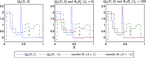
Figure 1: Plots for: the conditional mean function $Q_{0}(X,A)$ (left), $Q_{0}(X,A)$ and the associated best wavelet fit when $J_{n}=8$ (middle), and $Q_{0}(X,A)$ and the associated best wavelet fit when $J_{n}=128$ (right) [example (4)].

For each example, we simulate data sets of sizes $n=2^{k}$ for $k=5,\ldots,10$. $1\mbox{,}000$ data sets are generated for each sample size. The Value of each estimated ITR is evaluated via Monte Carlo using a test set of size $10\mbox{,}000$. The Value of the optimal ITR is also evaluated using the test set.

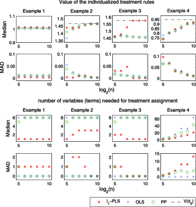
Figure 2: Comparison of the $l_{1}$-PLS based method with the OLS method and the PP method [examples (1)–(4)]: plots for medians and median absolute deviations (MAD) of the Value of the estimated decision rules (top panels) and the number of variables (terms) needed for treatment assignment (including the main treatment effect term, bottom panels) over $1\mbox{,}000$ samples versus sample size on the log scale. The black dash-dotted line in each plot on the first row denotes the Value of the optimal treatment rule, for each example. [$n=32,64,128,256,512,1024$. The corresponding numbers of basis functions in example (4) are $J_{n}=8,16,32,64,64,128$.]

Simulation results are presented in Figure 2. When the approximation model is of high quality, all methods produce ITRs with similar Value [see examples (1), (2) and example (4) for large $n$]. However, when the approximation model is poor, the $l_{1}$-PLS method may produce highest Value [see example (3)]. Note that in example (3) settings in which the sample size is small, the Value of the ITR produced by $l_{1}$-PLS method has larger median absolute deviation (MAD) than the other two methods. One possible reason is that due to the mismatch between maximizing the Value and minimizing the prediction error, the Value estimator plays a strong role in selecting $\lambda_{n}$. The nonsmoothness of the Value estimator combined with the mismatch results in very different $\lambda_{n}$’s and thus the estimated decision rules vary greatly from data set to data set in this example. Nonetheless, the $l_{1}$-PLS method is still preferred after taking the variation into account; indeed $l_{1}$-PLS produces ITRs with higher Value than both OLS and PP in around $46\%$, $55\%$ and $67\%$ in data sets of sizes $n=32,64$ and $128$, respectively. Furthermore, in general the $l_{1}$-PLS method uses much fewer variables for treatment assignment than the other two methods. This is expected because the OLS method does not have variable selection functionality and the PP method will use all variables that are predictive of the response $R$ whereas the use of the Value in selecting the tuning parameter in $l_{1}$-PLS discounts variables that are only useful in predicting the response (and less useful in selecting the best treatment).

5.2 Nefazodone-CBASP trial example

The Nefazodone-CBASP trial was conducted to compare the efficacy of several alternate treatments for patients with chronic depression. The study randomized $681$ patients with nonpsychotic chronic major depressive disorder (MDD) to either Nefazodone, cognitive behavioral-analysis system of psychotherapy (CBASP) or the combination of the two treatments. Various assessments were taken throughout the study, among which the score on the 24-item Hamilton Rating Scale for Depression (HRSD) was the primary outcome. Low HRSD scores are desirable. See Keller et al. keller2000 for more detail of the study design and the primary analysis.

In the data analysis, we use a subset of the Nefazodone-CBASP data consisting of $656$ patients for whom the response HRSD score was observed. In this trial, pairwise comparisons show that the combination treatment resulted in significantly lower HRSD scores than either of the single treatments. There was no overall difference between the single treatments.

We use $l_{1}$-PLS to develop an ITR. In the analysis, the HRSD score is reverse coded so that higher is better. We consider $50$ pretreatment variables $X=(X_{1},\ldots,X_{50})$. Treatments are coded using contrast coding of dummy variables $A=(A_{1},A_{2})$, where $A_{1}=2$ if the combination treatment is assigned and $-1$ otherwise and $A_{2}=1$ if CBASP is assigned, $-1$ if nefazodone and $0$ otherwise. The vector of basis functions, $\Phi(X,A)$, is of the form $(1,X,A_{1},XA_{1},A_{2},XA_{2})$. So the number of basis functions is $J=153$. As a contrast, we also consider the OLS method and the PP method (separate prognosis prediction for each treatment). The vector of basis functions used in PP is $(1,X)$ for each of the three treatment groups. Neither the intercept term nor the main treatment effect terms in $l_{1}$-PLS or PP is penalized (see Section S.2 of the supplemental article supplement for the modification of the weights $\hat{\sigma}_{j}$ used in (8)).

The ITR given by the $l_{1}$-PLS method recommends the combination treatment to all (so none of the pretreatment variables enter the rule). On the other hand, the PP method produces an ITR that uses $29$ variables. If the rule produced by PP were used to assign treatment for the $656$ patients in the trial, it would recommend the combination treatment for $614$ patients and nefazodone for the other $42$ patients. In addition, the OLS method will use all the $50$ variables. If the ITR produced by OLS were used to assign treatment for the $656$ patients in the trial, it would recommend the combination treatment for $429$ patients, nefazodone for $145$ patients and CBASP for the other $82$ patients.

6 Discussion

Our goal is to construct a high quality ITR that will benefit future patients. We considered an $l_{1}$-PLS based method and provided a finite sample upper bound for $V(d_{0})-V(\hat{d}_{n})$, the reduction in Value of the estimated ITR.

The use of an $l_{1}$ penalty allows us to consider a large model for the conditional mean function $Q_{0}$ yet permits a sparse estimated ITR. In fact, many other penalization methods such as SCAD fan2001 and $l_{1}$ penalty with adaptive weights (adaptive Lasso; zou2006 ) also have this property. We choose the nonadaptive $l_{1}$ penalty to represent these methods. Interested readers may justify other PLS methods using similar proof techniques.

The high probability finite sample upper bounds [i.e., (14) and (4.2)] cannot be used to construct a prediction/confidence interval for $V(d_{0})-V(\hat{d}_{n})$ due to the unknown quantities in the bound. How to develop a tight computable upper bound to assess the quality of $\hat{d}_{n}$ is an open question.

We used cross validation with Value maximization to select the tuning parameter involved in the $l_{1}$-PLS method. As compared to the OLS method and the PP method, this method may yield higher Value when $T_{0}$ is misspecified. However, since only the Value is used to select the tuning parameter, this method may produce a complex ITR for which the Value is only slightly higher than that of a much simpler ITR. In this case, a simpler rule may be preferred due to the interpretability and cost of collecting the variables. Investigation of a tuning parameter selection criterion that trades off the Value with the number of variables in an ITR is needed.

This paper studied a one stage decision problem. However, it is evident that some diseases require time-varying treatment. For example, individuals with a chronic disease often experience a waxing and waning course of illness. In these settings, the goal is to construct a sequence of ITRs that tailor the type and dosage of treatment through time according to an individual’s changing status. There is an abundance of statistical literature in this area thall2000 , thall2002 , murphy2003 , murphy2005 , robins2004 , lunceford2002 , vanderlaan2005 , wahedtsiatis2006 . Extension of the least squares based method to the multi-stage decision problem has been presented in Murphy murphy2005 . The performance of $l_{1}$ penalization in this setting is unclear and worth investigation.

Appendix

.1 Proof of Theorem 3.1

For any ITR $d\dvtx\mathcal{X}\rightarrow\mathcal{A}$, denote $\triangle T_{d}(X)$ $\triangleq\max_{a\in\mathcal{A}}T_{0}(X,a)-T_{0}(X,d(X))$. Using similar arguments to that in Section 2, we have $V(d_{0})-V(d)=E(\triangle T_{d})$. If $V(d_{0})-V(d)=0$, then (5) and (6) automatically hold. Otherwise, $E(\triangle T_{d})^{2}\geq(E\triangle T_{d})^{2}>0$. In this case, for any $\epsilon>0$, define the event

$$\Omega_{\epsilon}=\Bigl{\{}\max_{a\in\mathcal{A}}T_{0}(X,a)-\max_{a\in\mathcal{A}\setminus\mathop{\arg\max}_{a\in\mathcal{A}}T_{0}(X,a)}T_{0}(X,a)\leq\epsilon\Bigr{\}}.$$

Then $\triangle T_{d}\leq(\triangle T_{d})^{2}/\epsilon$ on the event $\Omega_{\epsilon}^{C}$. This together with the fact that $\triangle T_{d}\leq(\triangle T_{d})^{2}/\epsilon+\epsilon/4$ implies

$$V(d_{0})-V(d) = E(1_{\Omega_{\epsilon}^{C}}\triangle T_{d})+E(1_{\Omega_{\epsilon}}\triangle T_{d})$$

$$\leq \frac{1}{\epsilon}E[1_{\Omega_{\epsilon}^{C}}(\triangle T_{d})^{2}]+E\biggl{[}1_{\Omega_{\epsilon}}\biggl{(}\frac{(\triangle T_{d})^{2}}{\epsilon}+\frac{\epsilon}{4}\biggr{)}\biggr{]}$$

$$= \frac{1}{\epsilon}E[(\triangle T_{d})^{2}]+\frac{\epsilon}{4}P(\Omega_{\epsilon})\leq\frac{1}{\epsilon}E[(\triangle T_{d})^{2}]+\frac{C}{4}\epsilon^{1+\alpha},$$

where the last inequality follows from the margin condition (4). Choosing $\epsilon=(4E(\triangle T_{d})^{2}/C)^{1/(2+\alpha)}$ to minimize the above upper bound yields

$$V(d_{0})-V(d)\leq 2^{\alpha/(2+\alpha)}C^{1/(2+\alpha)}[E(\triangle T_{d})^{2}]^{(1+\alpha)/(2+\alpha)}.$$ (21)

Next, for any $d$ and $Q$ such that $d(X)\in\max_{a\in\mathcal{A}}Q(X,a)$, let $T(X,A)$ be the associated treatment effect term. Then

$$E(\triangle T_{d})^{2} = E\Bigl{[}\Bigl{(}\max_{a\in\mathcal{A}}T_{0}(X,a)-\max_{a\in\mathcal{A}}T(X,a)+T(X,d(X))-T_{0}(X,d(X))\Bigr{)}^{2}\Bigr{]}$$

$$\leq 2E\Bigl{[}\Bigl{(}\max_{a\in\mathcal{A}}T_{0}(X,a)-\max_{a\in\mathcal{A}}T(X,a)\Bigr{)}^{2}$$

$$\hskip 17.8pt{}+\bigl{(}T(X,d(X))-T_{0}(X,d(X))\bigr{)}^{2}\Bigr{]}$$

$$\leq 4E\Bigl{[}\max_{a\in\mathcal{A}}\bigl{(}T(X,a)-T_{0}(X,a)\bigr{)}^{2}\Bigr{]},$$

where the last inequality follows from the fact that neither $|{\max_{a}T_{0}(X,a)}-\max_{a}T(X,a)|$ nor $|T(X,d(X))-T_{0}(X,d(X))|$ is larger than ${\max_{a}}|T(X,a)-T_{0}(X,a)|$. Since $p(a|x)\geq S^{-1}$ for all $(x,a)$ pairs, we have

$$E(\triangle T_{d})^{2} \leq 4SE\Bigl{[}\sum_{a\in\mathcal{A}}\bigl{(}T(X,a)-T_{0}(X,a)\bigr{)}^{2}p(a|X)\Bigr{]}$$ (22)

$$= 4SE\bigl{(}T(X,A)-T_{0}(X,A)\bigr{)}^{2}.$$

Inequality (6) follows by substituting (22) into (21). Inequality (5) can be proved similarly by noticing that $\triangle T_{d}(X)=\max_{a\in\mathcal{A}}Q_{0}(X,a)-Q_{0}(X,d(X))$.

.2 Generalization of Theorem 4.3

In this section, we present a generalization of Theorem 4.3 where $J$ may depend on $n$ and the sparsity of any $\bolds{\theta}\in\mathbb{R}^{J}$ is measured by the number of “large” components in $\bolds{\theta}$ as described in Zhang and Huang chzhang2008 . In this case, $J$, $\Phi$ and the prediction error minimizer $\bolds{\theta}^{*}$ are denoted as $J_{n},\Phi_{n}$ and $\bolds{\theta}^{*}_{n}$, respectively. All relevant quantities and assumptions are restated below.

Let $|M|$ denote the cardinality of any index set $M\subseteq\{1,\ldots,J_{n}\}$. For any $\bolds{\theta}\in\mathbb{R}^{J_{n}}$ and constant $\rho\geq 0$, define

$$M_{\rho\lambda_{n}}(\bolds{\theta})\in\mathop{\arg\min}_{\{M\subseteq\{1,\ldots,J_{n}\}\dvtx\sum_{j\in\{1,\ldots,J_{n}\}\setminus M}\sigma_{j}|\theta_{j}|\leq\rho|M|\lambda_{n}\}}|M|.$$

Then $M_{\rho\lambda_{n}}(\bolds{\theta})$ is the smallest index set that contains only “large” components in $\bolds{\theta}$. $|M_{\rho\lambda_{n}}(\bolds{\theta})|$ measures the sparsity of $\bolds{\theta}$. It is easy to see that when $\rho=0$, $M_{0}(\bolds{\theta})$ is the index set of nonzero components in $\bolds{\theta}$ and $|M_{0}(\bolds{\theta})|=\|\bolds{\theta}\|_{0}$. Moreover, $M_{\rho\lambda_{n}}(\bolds{\theta})$ is an empty set if and only if $\bolds{\theta}=\mathbf{0}$.

Let $[\bolds{\theta}^{*}_{n}]$ be the set of most sparse prediction error minimizers in the linear model, that is,

$$[\bolds{\theta}^{*}_{n}]=\mathop{\arg\min}_{\bolds{\theta}\in\mathop{\arg\min}_{\bolds{\theta}}L(\Phi_{n}\bolds{\theta})}|M_{\rho\lambda_{n}}(\bolds{\theta})|.$$ (23)

Note that $[\bolds{\theta}^{*}_{n}]$ depends on $\rho\lambda_{n}$.

To derive the finite sample upper bound for $L(\Phi_{n}\bolds{\hat{\theta}}_{n})$, we need the following assumptions.

Assumption .1.

The error terms $\varepsilon_{i},i=1,\ldots,n$ are independent of $(X_{i},A_{i}),i=1,\ldots,n$ and are i.i.d. with $E(\varepsilon_{i})=0$ and $E[|\varepsilon_{i}|^{l}]\leq\frac{l!}{2}c^{l-2}\sigma^{2}$ for some $c,\sigma^{2}>0$ for all $l\geq 2$.

Assumption .2.

For all $n\geq 1$:

[(a)]

there exists an $1\leq U_{n}<\infty$ such that $\max_{j=1,\ldots,{J_{n}}}\|\phi_{j}\|_{\infty}/\sigma_{j}\leq U_{n}$, where $\sigma_{j}\triangleq(E\phi_{j}^{2})^{1/2}$.

there exists an $0<\eta_{1,n}<\infty$, such that $\sup_{\bolds{\theta}\in[\bolds{\theta}^{*}_{n}]}\|Q_{0}-\Phi_{n}\bolds{\theta}\|_{\infty}\leq\eta_{1,n}$.

For any $0\leq\gamma<1/2$, $\eta_{2,n}\geq 0$ (which may depend on $n$) and tuning parameter $\lambda_{n}$, define

$$\Theta_{n}^{o} = \biggl{\{}\bolds{\theta}\in\mathbb{R}^{J_{n}}\dvtx\exists\bolds{\theta}^{o}\in[\bolds{\theta}^{*}_{n}]\mbox{ s.t. }\|\Phi_{n}(\bolds{\theta}-\bolds{\theta}^{o})\|_{\infty}\leq\eta_{2,n}$$

$$\hskip 31.13pt\mbox{ and }\max_{j=1,\ldots,J_{n}}\biggl{|}E\biggl{[}\Phi_{n}(\bolds{\theta}-\bolds{\theta}^{o})\frac{\phi_{j}}{\sigma_{j}}\biggr{]}\biggr{|}\leq\gamma{\lambda_{n}}\biggr{\}}.$$

Assumption .3.

For any $n\geq 1$, there exists a $\beta_{n}>0$ such that

$$E[\Phi_{n}(\bolds{\tilde{\theta}}-\bolds{\theta})]^{2}|M_{\rho\lambda_{n}}(\bolds{\theta})|\geq\beta_{n}\biggl{[}\biggl{(}\sum_{j\in M_{\rho\lambda_{n}}(\bolds{\theta})}\sigma_{j}|\tilde{\theta}_{j}-\theta_{j}|\biggr{)}^{2}-\rho^{2}|M_{\rho\lambda_{n}}(\bolds{\theta})|^{2}\lambda_{n}^{2}\biggr{]}$$

for all $\bolds{\theta}\in\Theta_{n}^{o}\setminus\{\mathbf{0}\}$, $\bolds{\tilde{\theta}}\in\mathbb{R}^{J_{n}}$ satisfying $\sum_{j\in\{1,\ldots,J_{n}\}\setminus M_{\rho\lambda_{n}}(\bolds{\theta})}\sigma_{j}|\tilde{\theta}_{j}|\leq\frac{2\gamma+5}{1-2\gamma}\times(\sum_{j\in M_{\rho\lambda_{n}}(\bolds{\theta})}\sigma_{j}|\tilde{\theta}_{j}-\theta_{j}|+\rho|M_{\rho\lambda_{n}}(\bolds{\theta})|\lambda_{n})$.

When $E(\Phi_{n}^{(2)}(X,A)^{T}|X)=\mathbf{0}$ a.s. ($\Phi_{n}^{(2)}$ is defined in Section 4.1), we need an extra assumption to derive the finite sample upper bound for the mean square error of the treatment effect estimator $E[\Phi_{n}^{(2)}\bolds{\hat{\theta}}{}^{(2)}_{n}-T_{0}(X,A)]^{2}$ (recall that $T_{0}(X,A)\triangleq Q_{0}(X,A)-E[Q_{0}(X,A)|X]$).

Assumption .4.

For any $n\geq 1$, there exists a $\beta_{n}>0$ such that

$$E\bigl{[}\Phi_{n}^{(2)}\bigl{(}\bolds{\tilde{\theta}}{}^{(2)}-\bolds{\theta}^{(2)}\bigr{)}\bigr{]}^{2}\bigl{|}M_{\rho\lambda_{n}}^{(2)}(\bolds{\theta})\bigr{|}$$

$$\qquad\geq\beta_{n}\biggl{[}\biggl{(}\sum_{j\in M_{\rho\lambda_{n}}^{(2)}(\bolds{\theta})}\sigma_{j}|\tilde{\theta}_{j}-\theta_{j}|\biggr{)}^{2}-\rho^{2}\bigl{|}M_{\rho\lambda_{n}}^{(2)}(\bolds{\theta})\bigr{|}^{2}\lambda_{n}^{2}\biggr{]}$$

for all $\bolds{\theta}\in\Theta_{n}^{o}\setminus\{\mathbf{0}\}$, $\bolds{\tilde{\theta}}\in\mathbb{R}^{J_{n}}$ satisfying $\sum_{j\in\{1,\ldots,J_{n}\}\setminus M_{\rho\lambda_{n}}(\bolds{\theta})}\sigma_{j}|\tilde{\theta}_{j}|\leq\frac{2\gamma+5}{1-2\gamma}\times(\sum_{j\in M_{\rho\lambda_{n}}(\bolds{\theta})}|\tilde{\theta}_{j}-\theta_{j}|+\rho|M_{\rho\lambda_{n}}(\bolds{\theta})|\lambda_{n})$, where

$$M_{\rho\lambda_{n}}^{(2)}(\bolds{\theta})\in\mathop{\arg\min}_{\{M\subseteq\{J_{n}^{(1)}+1,\ldots,J_{n}\}\dvtx\sum_{j\in\{J_{n}^{(1)}+1,\ldots,J_{n}\}\setminus M}\sigma_{j}|\theta_{j}|\leq\rho|M|\lambda_{n}\}}|M|$$

is the smallest index set that contains only large components in $\bolds{\theta}^{(2)}$.

Without loss of generality, we assume that Assumptions .3 and .4 hold with the same value of $\beta_{n}$. And we can always choose a small enough $\beta_{n}$ so that $\rho\beta_{n}\leq 1$ for a given $\rho$.

For any given $t>0$, define

$$\Theta_{n} = \Biggl{\{}\bolds{\theta}\in\Theta_{n}^{o}\dvtx|M_{\rho\lambda_{n}}(\bolds{\theta})|$$

$$\hskip 6.5pt\leq\frac{(1-2\gamma)^{2}\beta_{n}}{120}\Biggl{[}\sqrt{\frac{1}{9}+\frac{n}{2U_{n}^{2}[\log(3J_{n}(J_{n}+1))+t]}}-\frac{1}{3}\Biggr{]}\Biggr{\}}.$$

Note that we allow $U_{n},\eta_{1,n},\eta_{2,n}$ and $\beta_{n}^{-1}$ to increase as $n$ increases. However, if those quantities are small, the upper bound in (27) will be tighter.

Theorem .1

Suppose Assumptions .1 and .2 hold. For any given $0\leq\gamma<1/2$, $\eta_{2,n}>0$, $\rho\geq 0$ and $t>0$, let $\bolds{\hat{\theta}}_{n}$ be the $l_{1}$-PLS estimator defined in (8) with tuning parameter

$$\lambda_{n} \geq \frac{8\max\{3c,2(\eta_{1,n}+\eta_{2,n})\}U_{n}(\log 6J_{n}+t)}{(1-2\gamma)n}$$

$${}+\frac{12\max\{\sigma,(\eta_{1,n}+\eta_{2,n})\}}{(1-2\gamma)}\sqrt{\frac{2(\log 6J_{n}+t)}{n}}.$$

Suppose Assumption .3 holds with $\rho\beta_{n}\leq 1$. Let $\Theta_{n}$ be the set defined in (.2) and assume $\Theta_{n}$ is nonempty. If

$$\frac{\log 2J_{n}}{n}\leq\frac{2(1-2\gamma)^{2}}{27U_{n}^{2}-10\gamma-22},$$ (26)

then with probability at least $1-\exp(-k^{\prime}_{n}n)-\exp(-t)$, we have

$$L(\Phi_{n}\bolds{\hat{\theta}}_{n})\leq\min_{\bolds{\theta}\in\Theta_{n}}\biggl{[}L(\Phi_{n}\bolds{\theta})+K_{n}\frac{|M_{\rho\lambda_{n}}(\bolds{\theta})|}{\beta_{n}}\lambda_{n}^{2}\biggr{]},$$ (27)

where $k_{n}^{\prime}=13(1-2\gamma)^{2}/[6(27U_{n}^{2}-10\gamma-22)]$ and $K_{n}=[40\gamma(12\beta_{n}\rho+2\gamma+5)]/[(1-2\gamma)(2\gamma+19)]+130(12\beta_{n}\rho+2\gamma+5)^{2}/[9(2\gamma+19)^{2}]$.

Furthermore, suppose $E(\Phi_{n}^{(2)}(X,A)^{T}|X)=\mathbf{0}$ a.s. If Assumption .4 holds with the same $\beta_{n}$ as that in Assumption .3, then with probability at least $1-\exp(-k^{\prime}_{n}n)-\exp(-t)$, we have

$$E\bigl{(}\Phi_{n}^{(2)}\bolds{\hat{\theta}}{}^{(2)}_{n}-T_{0}\bigr{)}^{2}\leq\min_{\bolds{\theta}\in\Theta_{n}}\biggl{[}E\bigl{(}\Phi_{n}^{(2)}\bolds{\theta}^{(2)}-T_{0}\bigr{)}^{2}+K^{\prime}_{n}\frac{|M_{\rho\lambda_{n}}^{(2)}(\bolds{\theta})|}{\beta_{n}}\lambda_{n}^{2}\biggr{]},$$

where $K_{n}^{\prime}=20(12\beta_{n}\rho+2\gamma+5)\{\gamma/[(1-2\gamma)(7-6\beta_{n}\rho)]+[3(1-2\gamma)\beta_{n}\rho+10(2\gamma+5)]/[9(2\gamma+19)^{2}]\}$.

[(1)]

Note that $K_{n}$ is upper bounded by a constant under the assumption $\beta_{n}\rho\leq 1$. In the asymptotic setting when $n\rightarrow\infty$ and $J_{n}\rightarrow\infty$, (27) implies that $L(\Phi_{n}\bolds{\hat{\theta}}_{n})-\min_{\bolds{\theta}\in\mathbb{R}^{J_{n}}}L(\Phi_{n}\bolds{\theta})\rightarrow^{p}0$ if (i) $|M_{\rho\lambda_{n}}(\bolds{\theta}^{o})|\lambda_{n}^{2}/\beta_{n}=o(1)$, (ii) $U_{n}^{2}\log J_{n}/n\leq k_{1}$ and $|M_{\rho\lambda_{n}}(\bolds{\theta}^{o})|\leq k_{2}\beta_{n}\sqrt{n/(U_{n}^{2}\log J_{n})}$ for some sufficiently small positive constants $k_{1}$ and $k_{2}$ and (iii) $\lambda_{n}\geq k_{3}\max\{1,\eta_{1,n}+\eta_{2,n}\}\sqrt{\log J_{n}/n}$ for a sufficiently large constant $k_{3}$, where $\bolds{\theta}^{o}\in[\bolds{\theta}^{*}_{n}]$ (take $t=\log J_{n}$).

Below we briefly discuss Assumptions .2–.4.

Assumption .2 is very similar to assumption (2) in Theorem 4.1 (which is used to prove the concentration of the sample mean around the true mean), except that $U_{n}$ and $\eta_{1,n}$ may increase as $n$ increases. This relaxation allows the use of basis functions for which the sup norm $\max_{j}\|\phi_{j}\|_{\infty}$ is increasing in $n$ [e.g., the wavelet basis used in example (4) of the simulation studies].

Assumption .3 is a generalization of condition (15) [which has been discussed in remark (4) following Theorem 4.1] to the case where $J_{n}$ may increase in $n$ and the sparsity of a parameter is measured by the number of “large” components as described at the beginning of this section. This condition is used to avoid the collinearity problem. It is easy to see that when $\rho=0$ and $\beta_{n}$ is fixed in $n$, this assumption simplifies to condition (15).

Assumption .4 puts a strengthened constraint on the linear model of the treatment effect part, as compared to Assumption .3. This assumption, together with Assumption .3, is needed in deriving the upper bound for the mean square error of the treatment effect estimator. It is easy to verify that if $E[\Phi_{n}^{T}\Phi_{n}]$ is positive definite, then both Assumptions .3 and .4 hold. Although the result is about the treatment effect part, which is asymptotically independent of the main effect of $X$ (when $E[\Phi_{n}^{(2)}(X,A)|X]=\mathbf{0}$ a.s.), we still need Assumption .3 to show that the cross product term $E_{n}[(\Phi_{n}^{(1)}\bolds{\hat{\theta}}{}^{(1)}_{n}-\Phi^{(1)}_{n}\bolds{\theta}^{(1)})(\Phi^{(2)}_{n}\bolds{\hat{\theta}}{}^{(2)}_{n}-\Phi^{(2)}_{n}\bolds{\theta}^{(2)})]$ is upper bounded by a quantity converging to $0$ at the desired rate. We may use a really poor model for the main effect part $E(Q_{0}(X,A)|X)$ (e.g., $\Phi^{(1)}_{n}\equiv 1$), and Assumption .4 implies Assumption .3 when $\rho=0$. This poor model only effects the constants involved in the result. When the sample size is large (so that $\lambda_{n}$ is small), the estimated ITR will be of high quality as long as $T_{0}$ is well approximated. Proof of Theorem .1 For any $\bolds{\theta}\in\Theta_{n}$, define the events

$$\Omega_{1} = \bigcap_{j=1}^{J_{n}}\biggl{\{}\frac{2(1+\gamma)}{3}\sigma_{j}\leq\hat{\sigma}_{j}\leq\frac{2(2-\gamma)}{3}\sigma_{j}\biggr{\}}\qquad\mbox{[where }\hat{\sigma}_{j}\triangleq(E_{n}\phi_{j}^{2})^{1/2}\mbox{]},$$

$$\Omega_{2}(\bolds{\theta}) = \biggl{\{}\max_{j,k=1,\ldots,{J_{n}}}\biggl{|}(E-E_{n})\biggl{(}\frac{\phi_{j}\phi_{k}}{\sigma_{j}\sigma_{k}}\biggr{)}\biggr{|}\leq\frac{(1-2\gamma)^{2}\beta_{n}}{120|M_{\rho\lambda_{n}}(\bolds{\theta})|}\biggr{\}},$$

$$\Omega_{3}(\bolds{\theta}) = \biggl{\{}\max_{j=1,\ldots,{J_{n}}}\biggl{|}E_{n}\biggl{[}(R-\Phi_{n}\bolds{\theta})\frac{\phi_{j}}{\sigma_{j}}\biggr{]}\biggr{|}\leq\frac{4\gamma+1}{6}\lambda_{n}\biggr{\}}.$$

Then there exists a $\bolds{\theta}^{o}\in[\bolds{\theta}^{*}_{n}]$ such that

$$L(\Phi_{n}\bolds{\hat{\theta}}_{n}) = L(\Phi_{n}\bolds{\theta})+2E[(\Phi_{n}\bolds{\theta}^{o}-\Phi_{n}\bolds{\theta})\Phi_{n}(\bolds{\theta}-\bolds{\hat{\theta}}_{n})]+E[\Phi_{n}(\bolds{\hat{\theta}}_{n}-\bolds{\theta})]^{2}$$

$$\leq L(\Phi_{n}\bolds{\theta})+2\max_{j=1,\ldots,J_{n}}\biggl{|}E\biggl{[}\Phi_{n}(\bolds{\theta}^{o}-\bolds{\theta})\frac{\phi_{j}}{\sigma_{j}}\biggr{]}\biggr{|}\Biggl{(}\sum_{j=1}^{J_{n}}\sigma_{j}|\hat{\theta}_{n,j}-\theta_{j}|\Biggr{)}$$

$${}+E[\Phi_{n}(\bolds{\hat{\theta}}_{n}-\bolds{\theta})]^{2}$$

$$\leq L(\Phi_{n}\bolds{\theta})+2\gamma\lambda_{n}\Biggl{(}\sum_{j=1}^{J_{n}}\sigma_{j}|\hat{\theta}_{n,j}-\theta_{j}|\Biggr{)}+E[\Phi_{n}(\bolds{\hat{\theta}}_{n}-\bolds{\theta})]^{2},$$

where the first equality follows from the fact that $E[(R-\Phi_{n}\bolds{\theta}^{o})\phi_{j}]=0$ for any $\bolds{\theta}^{o}\in[\bolds{\theta}^{*}_{n}]$ for $j=1,\ldots,J_{n}$ and the last inequality follows from the definition of $\Theta_{n}^{o}$.

Based on Lemma .1 below, we have that on the event $\Omega_{1}\cap\Omega_{2}(\bolds{\theta})\cap\Omega_{3}(\bolds{\theta})$,

$$L(\Phi_{n}\bolds{\hat{\theta}}_{n})\leq L(\Phi_{n}\bolds{\theta})+K_{n}\frac{|M_{\rho\lambda_{n}}(\bolds{\theta})|}{\beta_{n}}\lambda_{n}^{2}.\vspace{-2pt}$$

Similarly, when $E[\Phi^{(2)}_{2}(X,A)^{T}|X]=\mathbf{0}$, by Lemma .2, we have that on the event $\Omega_{1}\cap\Omega_{2}(\bolds{\theta})\cap\Omega_{3}(\bolds{\theta})$,

$$E\bigl{(}\Phi_{n}^{(2)}\bolds{\hat{\theta}}{}^{(2)}_{n}-T_{0}\bigr{)}^{2} \leq E\bigl{(}\Phi_{n}^{(2)}\bolds{\theta}^{(2)}-T_{0}\bigr{)}^{2}+2\gamma\lambda_{n}\Biggl{(}\sum_{j=J_{n}^{(1)}+1}^{J_{n}}\sigma_{j}|\hat{\theta}_{n,j}-\theta_{j}|\Biggr{)}$$

$${}+E\bigl{[}\Phi_{n}^{(2)}\bigl{(}\bolds{\hat{\theta}}{}^{(2)}_{n}-\bolds{\theta}^{(2)}\bigr{)}\bigr{]}^{2}$$

$$\leq E\bigl{(}\Phi_{n}^{(2)}\bolds{\theta}^{(2)}-T_{0}\bigr{)}^{2}+K^{\prime}_{n}\frac{|M_{\rho\lambda_{n}}^{(2)}(\bolds{\theta})|}{\beta_{n}}\lambda_{n}^{2}.$$

The conclusion of the theorem follows from the union probability bounds of the events $\Omega_{1}$, $\Omega_{2}(\bolds{\theta})$ and $\Omega_{3}(\bolds{\theta})$ provided in Lemmas .3, .4 and .5.

Below we state the lemmas used in the proof of Theorem .1. The proofs of the lemmas are given in Section S.4 of the supplemental article supplement .

Lemma .1

Suppose Assumption .3 holds with $\rho\beta_{n}\leq 1$. Then for any $\bolds{\theta}\in\Theta_{n}$, on the event $\Omega_{1}\cap\Omega_{2}(\bolds{\theta})\cap\Omega_{3}(\bolds{\theta})$, we have

$$\sum_{j=1}^{J_{n}}\sigma_{j}|\hat{\theta}_{n,j}-\theta_{j}|\leq\frac{20(12\rho\beta_{n}+2\gamma+5)}{(1-2\gamma)(19+2\gamma)\beta_{n}}|M_{\rho\lambda_{n}}(\bolds{\theta})|\lambda_{n}$$ (28)

and

$$E[\Phi_{n}(\bolds{\hat{\theta}}_{n}-\bolds{\theta})]^{2}\leq\frac{130(12\rho\beta_{n}+2\gamma+5)^{2}}{9(19+2\gamma)^{2}\beta_{n}}|M_{\rho\lambda_{n}}(\bolds{\theta})|\lambda_{n}^{2}$$ (29)

This lemma implies that $\bolds{\hat{\theta}}_{n}$ is close to each $\bolds{\theta}\in\Theta_{n}$ on the event $\Omega_{1}\cap\Omega_{2}(\bolds{\theta})\cap\Omega_{3}(\bolds{\theta})$. The intuition is as follows. Since $\bolds{\hat{\theta}}_{n}$ minimizes (8), the first order conditions imply that $\max_{j}|E_{n}(R-\Phi_{n}\bolds{\hat{\theta}}_{n})\phi_{j}/\hat{\sigma}_{j}|\leq\lambda_{n}/2$. Similar property holds for $\bolds{\theta}$ on the event $\Omega_{1}\cap\Omega_{3}(\bolds{\theta})$. Assumption .3 together with event $\Omega_{2}(\bolds{\theta})$ ensures that there is no collinearity in the $n\times J_{n}$ design matrix $(\Phi_{n}(X_{i},A_{i}))_{i=1}^{n}$. These two aspects guarantee the closeness of $\bolds{\hat{\theta}}_{n}$ to $\bolds{\theta}$.

Lemma .2

Suppose $E[\Phi_{n}^{(2)}(X,A)^{T}|X]=\mathbf{0}$ a.s. and Assumptions .3 and .4 hold with $\rho\beta_{n}\leq 1$. Then for any $\bolds{\theta}\in\Theta_{n}$, on the event $\Omega_{1}\cap\Omega_{2}(\bolds{\theta})\cap\Omega_{3}(\bolds{\theta})$, we have

$$\sum_{j=J_{n}^{(1)}+1}^{J_{n}}\sigma_{j}|\hat{\theta}_{n,j}-\theta_{j}|\leq\frac{10(12\beta_{n}\rho+2\gamma+5)}{(1-2\gamma)(7-6\beta_{n}\rho)\beta_{n}}\bigl{|}M_{\rho\lambda_{n}}^{(2)}(\bolds{\theta})\bigr{|}\lambda_{n}$$ (30)

and

$$E\bigl{[}\Phi_{n}^{(2)}\bigl{(}\bolds{\hat{\theta}}{}^{(2)}_{n}-\bolds{\theta}^{(2)}\bigr{)}\bigr{]}^{2}$$

$$\qquad\leq\frac{20(12\rho\beta_{n}+2\gamma+5)[3(1-2\gamma)\beta_{n}\rho+10(2\gamma+5)]}{9(2\gamma+19)^{2}\beta_{n}}\bigl{|}M_{\rho\lambda_{n}}^{(2)}(\bolds{\theta})\bigr{|}\lambda_{n}^{2}.$$

Lemma .3

Suppose Assumption .2(a) and inequality (26) hold. Then $\mathbf{P}(\Omega_{1}^{C})\leq\exp(-k^{\prime}_{n}n)$, where $k^{\prime}_{n}=13(1-2\gamma)^{2}/[6(27U_{n}^{2}-10\gamma-22)]$.

Lemma .4

Suppose Assumption .2(a) holds. Then for any $t>0$ and $\bolds{\theta}\in\Theta_{n}$, $\mathbf{P}(\{\Omega_{2}(\bolds{\theta})\}^{C})\leq\exp(-t)/3$.

Lemma .5

Suppose Assumptions .1 and .2 hold. For any $t>0$, if $\lambda_{n}$ satisfies condition (.1), then for any $\bolds{\theta}\in\Theta_{n}$, we have $\mathbf{P}(\{\Omega_{3}(\bolds{\theta})\}^{C})\leq 2\exp(-t)/3$.

.3 Design of simulations in Section 5.1

In this section, we present the detailed simulation design of the examples used in Section 5.1. These examples satisfy all assumptions listed in the theorems [it is easy to verify that for examples (1)–(3). Validity of the assumptions for example (4) is addressed in the remark after example (4)]. In addition, $\Theta_{n}$ defined in (4.1) is nonempty as long as $n$ is sufficiently large (note that the constants involved in $\Theta_{n}$ can be improved and are not that meaningful. We focused on a presentable result instead of finding the best constants).

In examples (1)–(3), $X=(X_{1},\ldots,X_{5})$ is uniformly distributed on $[-1,1]^{5}$. The treatment $A$ is then generated independently of $X$ uniformly from $\{-1,1\}$. Given $X$ and $A$, the response $R$ is generated from a normal distribution with mean $Q_{0}(X,A)=1+2X_{1}+X_{2}+0.5X_{3}+T_{0}(X,A)$ and variance $1$. We consider the following three examples for $T_{0}$: [(1)]

$T_{0}(X,A)=0$ (i.e., there is no treatment effect).

$T_{0}(X,A)=0.424(1-X_{1}-X_{2})A$.

$T_{0}(X,A)=0.446\operatorname{sign}(X_{1})(1-X_{1})^{2}A$. Note that in each example $T_{0}(X,A)$ is equal to the treatment effect term, $Q_{0}(X,A)-E[Q_{0}(X,A)|X]$. We approximate $Q_{0}$ by $\mathcal{Q}=\{(1,X,A,XA)\bolds{\theta}\dvtx\break\bolds{\theta}\in\mathbb{R}^{12}\}$. Thus, in examples (1) and (2) the treatment effect term $T_{0}$ is correctly modeled, while in example (3) the treatment effect term $T_{0}$ is misspecified.

The parameters in examples (2) and (3) are chosen to reflect a medium effect size according to Cohen’s d index. When there are two treatments, the Cohen’s d effect size index is defined as the standardized difference in mean responses between two treatment groups, that is,

$$\mathrm{es}=\frac{E(R|A=1)-E(R|A=-1)}{([\operatorname{Var}(R|A=1)+\operatorname{Var}(R|A=-1)]/2)^{1/2}}.$$

Cohen cohen1988 tentatively defined the effect size as “small” if the Cohen’s d index is $0.2$, “medium” if the index is $0.5$ and “large” if the index is $0.8$.

In example (4), $X$ is uniformly distributed on $[0,1]$. Treatment $A$ is generated independently of $X$ uniformly from $\{-1,1\}$. The response $R$ is generated from a normal distribution with mean $Q_{0}(X,A)$ and variance $1$, where $Q_{0}(X,1)=\sum_{j=1}^{8}\vartheta_{(1),j}1_{X<u_{(1),j}}$, $Q_{0}(X,-1)=\sum_{j=1}^{8}\vartheta_{(-1),j}1_{X<u_{(-1),j}}$, and $\vartheta$’s and $u$’s are parameters specified in (.3). The effect size is small:

$$\bigl{(}\vartheta_{(1),1},\ldots,\vartheta_{(1),8}\bigr{)}$$

$$\qquad=(-0.781,0.730,0.635,0.512,-2.278,1.347,1.155,-0.030);$$

$$\bigl{(}\vartheta_{(-1),1},\ldots,\vartheta_{(-1),8}\bigr{)}$$

$$\qquad=(-2.068,1.520,-0.072,$$

$$\hskip 37.7pt-0.637,1.003,-0.611,-0.305,1.016);$$

$$\bigl{(}u_{(1),1},\ldots,u_{(1),8}\bigr{)}$$

$$\qquad=(0.028,0.144,0.171,0.298,0.421,0.443,0.463,0.758);$$

$$\bigl{(}u_{(-1),1},\ldots,u_{(-1),8}\bigr{)}$$

$$\qquad=(0.061,0.215,0.492,0.544,0.6302,0.650,0.785,0.909).$$

We approximate $Q_{0}$ by Haar wavelets,

$$\theta_{(0),0}h_{0}(X)+\sum_{lk}\theta_{(0),lk}h_{lk}(X)+\biggl{(}\theta_{(0),1}h_{0}(X)+\sum_{lk}\theta_{(1),lk}h_{lk}(X)\biggr{)}A,$$

where $h_{0}(x)=1_{x\in[0,1]}$ and $h_{lk}(x)=2^{l/2}(1_{2^{l}x\in[k+1/2,k+1)}-1_{2^{l}x\in[k,k+1/2)})$ for $l=0,\ldots,\bar{l}_{n}$, and $\theta_{(\cdot),\cdot}\in\mathbb{R}$ are parameters. We choose $\bar{l}_{n}=\lfloor 3\log_{2}n/4\rfloor-2$. For a given $l$ and sample $(X_{i},A_{i},R_{i})_{i=1}^{n}$, $k$ takes integer values from $\lfloor 2^{l}\min_{i}X_{i}\rfloor$ to $\lceil 2^{l}\max_{i}X_{i}\rceil-1$. Then $J_{n}=2^{\lfloor 3\log_{2}n/4\rfloor}\leq n^{3/4}$.

In example (4), we allow the number of basis functions $J_{n}$ to increase with $n$. The corresponding theoretical result can be obtained by combining Theorems 3.1 and .1. Below we demonstrate the validation of the assumptions used in the theorems.

Theorem 3.1 requires that the randomization probability $p(a|x)\geq S^{-1}$ for a positive constant for all $(x,a)$ pairs and the margin condition (4) or (7) holds. According the generative model, we have that $p(a|x)=1/2$ and condition (7) holds.

Theorem .1 requires Assumptions .1–.4 hold and $\Theta_{n}$ defined in (.2) is nonempty. Since we consider normal error terms, Assumption .1 holds. Note that the basis functions used in Haar wavelet are orthogonal. It is also easy to verify that Assumptions .3 and .4 hold with $\beta_{n}=1$ and Assumption .2 holds with $U_{n}=n^{3/8}/2$ and $\eta_{1,n}\leq\mbox{constant}+\mbox{constant}\times\|\bolds{\theta}^{*}_{n}\|_{0}$ [since each $|\phi_{j}\bolds{\theta}^{*}_{n,j}|=|\phi_{j}E(\phi_{j}R)|\leq\mbox{constant}\times|\phi_{j}|E|\phi_{j}|\leq O(1)$]. Since $Q_{0}$ is piece-wise constant, we can also verify that $\|\bolds{\theta}^{*}_{n}\|_{0}\leq O(\log n)$. Thus, for sufficiently large $n$, $\Theta_{n}$ is nonempty and (26) holds. The RHS of (.1) converges to zero as $n\rightarrow\infty$.

References

- (1) {barticle}[mr] \bauthor\bsnmBartlett, \bfnmPeter L.\binitsP. L. (\byear2008). \btitleFast rates for estimation error and oracle inequalities for model selection. \bjournalEconometric Theory \bvolume24 \bpages545–552. \biddoi=10.1017/S0266466608080225, mr=2490397 \endbibitem
- (2) {barticle}[mr] \bauthor\bsnmBartlett, \bfnmPeter L.\binitsP. L., \bauthor\bsnmJordan, \bfnmM. L.\binitsM. L. and \bauthor\bsnmMcAuliffe, \bfnmP. L.\binitsP. L. (\byear2006). \btitleConvexity, classification, and risk bounds. \bjournalJ. Amer. Statist. Assoc. \bvolume101 \bpages138–156. \biddoi=10.1007/s00440-005-0462-3, mr=2268032 \endbibitem
- (3) {barticle}[mr] \bauthor\bsnmBickel, \bfnmPeter J.\binitsP. J., \bauthor\bsnmRitov, \bfnmYa’acov\binitsY. and \bauthor\bsnmTsybakov, \bfnmAlexandre B.\binitsA. B. (\byear2009). \btitleSimultaneous analysis of lasso and Dantzig selector. \bjournalAnn. Statist. \bvolume37 \bpages1705–1732. \biddoi=10.1214/08-AOS620, mr=2533469 \endbibitem
- (4) {barticle}[mr] \bauthor\bsnmBunea, \bfnmFlorentina\binitsF., \bauthor\bsnmTsybakov, \bfnmAlexandre\binitsA. and \bauthor\bsnmWegkamp, \bfnmMarten\binitsM. (\byear2007). \btitleSparsity oracle inequalities for the Lasso. \bjournalElectron. J. Stat. \bvolume1 \bpages169–194 (electronic). \biddoi=10.1214/07-EJS008, mr=2312149 \endbibitem
- (5) {bmisc}[auto:STB—2010-11-18—09:18:59] \bauthor\bsnmCai, \bfnmT.\binitsT., \bauthor\bsnmTian, \bfnmL.\binitsL., \bauthor\bsnmLloyd-Jones, \bfnmD. M.\binitsD. M. and \bauthor\bsnmWei, \bfnmL. J.\binitsL. J. (\byear2008). \bhowpublishedEvaluating subject-level incremental values of new markers for risk classification rule. Working Paper 91, Harvard Univ. Biostatistics Working Paper Series. \endbibitem
- (6) {barticle}[auto:STB—2010-11-18—09:18:59] \bauthor\bsnmCai, \bfnmT.\binitsT., \bauthor\bsnmTian, \bfnmL.\binitsL., \bauthor\bsnmUno, \bfnmH.\binitsH., \bauthor\bsnmSolomon, \bfnmS. D.\binitsS. D. and \bauthor\bsnmWei, \bfnmL. J.\binitsL. J. (\byear2010). \btitleCalibrating parametric subject-specific risk estimation. \bjournalBiometrika \bvolume97 \bpages389–404. \endbibitem
- (7) {bbook}[auto:STB—2010-11-18—09:18:59] \bauthor\bsnmCohen, \bfnmJ.\binitsJ. (\byear1988). \btitleStatistical Power Analysis for the Behavioral Sciences, \bedition2nd ed. \bpublisherLawrence Erlbaum Associates, \baddressHillsdale, NJ. \endbibitem
- (8) {barticle}[mr] \bauthor\bsnmDonoho, \bfnmDavid L.\binitsD. L. and \bauthor\bsnmJohnstone, \bfnmIain M.\binitsI. M. (\byear1994). \btitleIdeal spatial adaptation by wavelet shrinkage. \bjournalBiometrika \bvolume81 \bpages425–455. \biddoi=10.1093/biomet/81.3.425, mr=1311089 \endbibitem
- (9) {barticle}[mr] \bauthor\bsnmFan, \bfnmJianqing\binitsJ. and \bauthor\bsnmLi, \bfnmRunze\binitsR. (\byear2001). \btitleVariable selection via nonconcave penalized likelihood and its oracle properties. \bjournalJ. Amer. Statist. Assoc. \bvolume96 \bpages1348–1360. \biddoi=10.1198/016214501753382273, mr=1946581 \endbibitem
- (10) {barticle}[pbm] \bauthor\bsnmFeldstein, \bfnmM. L.\binitsM. L., \bauthor\bsnmSavlov, \bfnmE. D.\binitsE. D. and \bauthor\bsnmHilf, \bfnmR.\binitsR. (\byear1978). \btitleA statistical model for predicting response of breast cancer patients to cytotoxic chemotherapy. \bjournalCancer Res. \bvolume38 \bpages2544–2548. \bidpmid=667849 \endbibitem
- (11) {barticle}[pbm] \bauthor\bsnmInsel, \bfnmThomas R.\binitsT. R. (\byear2009). \btitleTranslating scientific opportunity into public health impact: A strategic plan for research on mental illness. \bjournalArch. Gen. Psychiatry \bvolume66 \bpages128–133. \bidpii=66/2/128, doi=10.1001/archgenpsychiatry.2008.540, pmid=19188534 \endbibitem
- (12) {bmisc}[auto:STB—2010-11-18—09:18:59] \bauthor\bsnmIshigooka, \bfnmJ.\binitsJ., \bauthor\bsnmMurasaki, \bfnmM.\binitsM. \bauthor\bsnmMiura, \bfnmS.\binitsS. and \borganizationThe Olanzapine Late-Phase II Study Group (\byear2011). \bhowpublishedOlanzapine optimal dose: Results of an open-label multicenter study in schizophrenic patients. Psychiatry and Clinical Neurosciences 54 467–478. \endbibitem
- (13) {barticle}[pbm] \bauthor\bsnmKeller, \bfnmM. B.\binitsM. B., \bauthor\bsnmMcCullough, \bfnmJ. P.\binitsJ. P., \bauthor\bsnmKlein, \bfnmD. N.\binitsD. N., \bauthor\bsnmArnow, \bfnmB.\binitsB., \bauthor\bsnmDunner, \bfnmD. L.\binitsD. L., \bauthor\bsnmGelenberg, \bfnmA. J.\binitsA. J., \bauthor\bsnmMarkowitz, \bfnmJ. C.\binitsJ. C., \bauthor\bsnmNemeroff, \bfnmC. B.\binitsC. B., \bauthor\bsnmRussell, \bfnmJ. M.\binitsJ. M., \bauthor\bsnmThase, \bfnmM. E.\binitsM. E., \bauthor\bsnmTrivedi, \bfnmM. H.\binitsM. H. and \bauthor\bsnmZajecka, \bfnmJ.\binitsJ. (\byear2000). \btitleA comparison of nefazodone, the cognitive behavioral-analysis system of psychotherapy, and their combination for the treatment of chronic depression. \bjournalN. Engl. J. Med. \bvolume342 \bpages1462–1470. \bidpmid=10816183, doi=10.1056/NEJM200005183422001 \endbibitem
- (14) {barticle}[pbm] \bauthor\bsnmKent, \bfnmDavid M.\binitsD. M., \bauthor\bsnmHayward, \bfnmRodney A.\binitsR. A., \bauthor\bsnmGriffith, \bfnmJohn L.\binitsJ. L., \bauthor\bsnmVijan, \bfnmSandeep\binitsS., \bauthor\bsnmBeshansky, \bfnmJoni R.\binitsJ. R., \bauthor\bsnmCaliff, \bfnmRobert M.\binitsR. M. and \bauthor\bsnmSelker, \bfnmHarry P.\binitsH. P. (\byear2002). \btitleAn independently derived and validated predictive model for selecting patients with myocardial infarction who are likely to benefit from tissue plasminogen activator compared with streptokinase. \bjournalAm. J. Med. \bvolume113 \bpages104–111. \bidpmid=12133748, pii=S0002934302011609 \endbibitem
- (15) {barticle}[mr] \bauthor\bsnmKoltchinskii, \bfnmVladimir\binitsV. (\byear2009). \btitleSparsity in penalized empirical risk minimization. \bjournalAnn. Inst. H. Poincaré Probab. Statist. \bvolume45 \bpages7–57. \biddoi=10.1214/07-AIHP146, mr=2500227 \endbibitem
- (16) {barticle}[pbm] \bauthor\bsnmLesko, \bfnmL. J.\binitsL. J. (\byear2007). \btitlePersonalized medicine: Elusive dream or imminent reality? \bjournalClin. Pharmacol. Ther. \bvolume81 \bpages807–816. \bidpii=6100204, doi=10.1038/sj.clpt.6100204, pmid=17505496 \endbibitem
- (17) {barticle}[mr] \bauthor\bsnmLunceford, \bfnmJared K.\binitsJ. K., \bauthor\bsnmDavidian, \bfnmMarie\binitsM. and \bauthor\bsnmTsiatis, \bfnmAnastasios A.\binitsA. A. (\byear2002). \btitleEstimation of survival distributions of treatment policies in two-stage randomization designs in clinical trials. \bjournalBiometrics \bvolume58 \bpages48–57. \biddoi=10.1111/j.0006-341X.2002.00048.x, mr=1891042 \endbibitem
- (18) {barticle}[mr] \bauthor\bsnmMammen, \bfnmEnno\binitsE. and \bauthor\bsnmTsybakov, \bfnmAlexandre B.\binitsA. B. (\byear1999). \btitleSmooth discrimination analysis. \bjournalAnn. Statist. \bvolume27 \bpages1808–1829. \biddoi=10.1214/aos/1017939240, mr=1765618 \endbibitem
- (19) {bincollection}[mr] \bauthor\bsnmMassart, \bfnmPascal\binitsP. (\byear2005). \btitleA non-asymptotic theory for model selection. In \bbooktitleEuropean Congress of Mathematics \bpages309–323. \bpublisherEur. Math. Soc., \baddressZürich. \bidmr=2185752 \endbibitem
- (20) {barticle}[mr] \bauthor\bsnmMurphy, \bfnmS. A.\binitsS. A. (\byear2003). \btitleOptimal dynamic treatment regimes. \bjournalJ. R. Stat. Soc. Ser. B Stat. Methodol. \bvolume65 \bpages331–366. \biddoi=10.1111/1467-9868.00389, mr=1983752 \endbibitem
- (21) {barticle}[mr] \bauthor\bsnmMurphy, \bfnmSusan A.\binitsS. A. (\byear2005). \btitleA generalization error for Q-learning. \bjournalJ. Mach. Learn. Res. \bvolume6 \bpages1073–1097 (electronic). \bidmr=2249849 \endbibitem
- (22) {barticle}[mr] \bauthor\bsnmMurphy, \bfnmS. A.\binitsS. A., \bauthor\bparticlevan der \bsnmLaan, \bfnmM. J.\binitsM. J., \bauthor\bsnmRobins, \bfnmJ. M.\binitsJ. M. and (\byear2001). \btitleMarginal mean models for dynamic regimes. \bjournalJ. Amer. Statist. Assoc. \bvolume96 \bpages1410–1423. \biddoi=10.1198/016214501753382327, mr=1946586 \endbibitem
- (23) {barticle}[auto:STB—2010-11-18—09:18:59] \bauthor\bsnmPiquette-Miller, \bfnmP.\binitsP. and \bauthor\bsnmGrant, \bfnmD. M.\binitsD. M. (\byear2007). \btitleThe art and science of personalized medicine. \bjournalClin. Pharmacol. Ther. \bvolume81 \bpages311–315. \endbibitem
- (24) {barticle}[mr] \bauthor\bsnmPolonik, \bfnmWolfgang\binitsW. (\byear1995). \btitleMeasuring mass concentrations and estimating density contour clusters—an excess mass approach. \bjournalAnn. Statist. \bvolume23 \bpages855–881. \biddoi=10.1214/aos/1176324626, mr=1345204 \endbibitem
- (25) {bmisc}[auto:STB—2010-11-18—09:18:59] \bauthor\bsnmQian, \bfnmM.\binitsM. and \bauthor\bsnmMurphy, \bfnmS. A.\binitsS. A. (\byear2011). \bhowpublishedSupplement to “Performance guarantees for individualized treatment rules.” DOI:10.1214/10-AOS864SUPP. \endbibitem
- (26) {barticle}[mr] \bauthor\bsnmRobins, \bfnmJames\binitsJ., \bauthor\bsnmOrellana, \bfnmLiliana\binitsL. and \bauthor\bsnmRotnitzky, \bfnmAndrea\binitsA. (\byear2008). \btitleEstimation and extrapolation of optimal treatment and testing strategies. \bjournalStat. Med. \bvolume27 \bpages4678–4721. \biddoi=10.1002/sim.3301, mr=2528576 \endbibitem
- (27) {binproceedings}[mr] \bauthor\bsnmRobins, \bfnmJames M.\binitsJ. M. (\byear2004). \btitleOptimal-regime structural nested models. In \bbooktitleProceedings of the Second Seattle Symposium on Biostatistics (\beditorD. Y. Lin and P. Haegerty eds.). \bpublisherSpringer, \baddressNew York. \endbibitem
- (28) {barticle}[pbm] \bauthor\bsnmStoehlmacher, \bfnmJ.\binitsJ., \bauthor\bsnmPark, \bfnmD. J.\binitsD. J., \bauthor\bsnmZhang, \bfnmW.\binitsW., \bauthor\bsnmYang, \bfnmD.\binitsD., \bauthor\bsnmGroshen, \bfnmS.\binitsS., \bauthor\bsnmZahedy, \bfnmS.\binitsS. and \bauthor\bsnmLenz, \bfnmH-J\binitsH.-J. (\byear2004). \btitleA multivariate analysis of genomic polymorphisms: Prediction of clinical outcome to 5-FU/oxaliplatin combination chemotherapy in refractory colorectal cancer. \bjournalBr. J. Cancer \bvolume91 \bpages344–354. \bidpmid=15213713, doi=10.1038/sj.bjc.6601975, pii=6601975, pmcid=2409815 \endbibitem
- (29) {barticle}[pbm] \bauthor\bsnmThall, \bfnmP. F.\binitsP. F., \bauthor\bsnmMillikan, \bfnmR. E.\binitsR. E. and \bauthor\bsnmSung, \bfnmH. G.\binitsH. G. (\byear2000). \btitleEvaluating multiple treatment courses in clinical trials. \bjournalStat. Med. \bvolume19 \bpages1011–1028. \bidpmid=10790677, pii=10.1002/(SICI)1097-0258(20000430)19:8¡1011::AID-SIM414¿3.0.CO;2-M \endbibitem
- (30) {barticle}[mr] \bauthor\bsnmThall, \bfnmPeter F.\binitsP. F., \bauthor\bsnmSung, \bfnmHsi-Guang\binitsH.-G. and \bauthor\bsnmEstey, \bfnmElihu H.\binitsE. H. (\byear2002). \btitleSelecting therapeutic strategies based on efficacy and death in multicourse clinical trials. \bjournalJ. Amer. Statist. Assoc. \bvolume97 \bpages29–39. \biddoi=10.1198/016214502753479202, mr=1947271 \endbibitem
- (31) {barticle}[mr] \bauthor\bsnmTibshirani, \bfnmRobert\binitsR. (\byear1996). \btitleRegression shrinkage and selection via the lasso. \bjournalJ. Roy. Statist. Soc. Ser. B \bvolume58 \bpages267–288. \bidmr=1379242 \endbibitem
- (32) {barticle}[mr] \bauthor\bsnmTsybakov, \bfnmAlexandre B.\binitsA. B. (\byear2004). \btitleOptimal aggregation of classifiers in statistical learning. \bjournalAnn. Statist. \bvolume32 \bpages135–166. \biddoi=10.1214/aos/1079120131, mr=2051002 \endbibitem
- (33) {barticle}[mr] \bauthor\bparticlevan de \bsnmGeer, \bfnmSara A.\binitsS. A. (\byear2008). \btitleHigh-dimensional generalized linear models and the lasso. \bjournalAnn. Statist. \bvolume36 \bpages614–645. \biddoi=10.1214/009053607000000929, mr=2396809 \endbibitem
- (34) {barticle}[mr] \bauthor\bparticlevan der \bsnmLaan, \bfnmMark J.\binitsM. J., \bauthor\bsnmPetersen, \bfnmMaya L.\binitsM. L. and \bauthor\bsnmJoffe, \bfnmMarshall M.\binitsM. M. (\byear2005). \btitleHistory-adjusted marginal structural models and statically-optimal dynamic treatment regimens. \bjournalInt. J. Biostat. \bvolume1 \bpagesArt. 4, 41 pp. (electronic). \bidmr=2232229 \endbibitem
- (35) {barticle}[mr] \bauthor\bsnmWahed, \bfnmAbdus S.\binitsA. S. and \bauthor\bsnmTsiatis, \bfnmAnastasios A.\binitsA. A. (\byear2006). \btitleSemiparametric efficient estimation of survival distributions in two-stage randomisation designs in clinical trials with censored data. \bjournalBiometrika \bvolume93 \bpages163–177. \biddoi=10.1093/biomet/93.1.163, mr=2277748 \endbibitem
- (36) {barticle}[mr] \bauthor\bsnmZhang, \bfnmCun-Hui\binitsC.-H. and \bauthor\bsnmHuang, \bfnmJian\binitsJ. (\byear2008). \btitleThe sparsity and bias of the LASSO selection in high-dimensional linear regression. \bjournalAnn. Statist. \bvolume36 \bpages1567–1594. \biddoi=10.1214/07-AOS520, mr=2435448 \endbibitem
- (37) {barticle}[mr] \bauthor\bsnmZou, \bfnmHui\binitsH. (\byear2006). \btitleThe adaptive lasso and its oracle properties. \bjournalJ. Amer. Statist. Assoc. \bvolume101 \bpages1418–1429. \biddoi=10.1198/016214506000000735, mr=2279469 \endbibitem