On the Mass of CoRoT-7b

Abstract

The mass of CoRoT-7b, the first transiting superearth exoplanet, is still a subject of debate. A wide range of masses have been reported in the literature ranging from as high as 8 $M_{\oplus}$ to as low as 2.3 $M_{\oplus}$. Although most mass determinations give a density consistent with a rocky planet, the lower value permits a bulk composition that can be up to 50% water. We present an analysis of the CoRoT-7b radial velocity measurements that uses very few and simple assumptions in treating the activity signal. By only analyzing those radial velocity data for which multiple measurements were made in a given night we remove the activity related radial velocity contribution without any a priori model. We demonstrate that the contribution of activity to the final radial velocity curve is negligible and that the $K$-amplitude due to the planet is well constrained. This yields a mass of 7.42 $\pm$ 1.21 $M_{\oplus}$ and a mean density of $\rho$ = 10.4 $\pm$ 1.8 gm cm^-3. CoRoT-7b is similar in mass and radius to the second rocky planet to be discovered, Kepler-10b, and within the errors they have identical bulk densities - they are virtual twins. These bulk densities lie close to the density - radius relationship for terrestrial planets similar to what is seen for Mercury. CoRoT-7b and Kepler-10b may have an internal structure more like Mercury than the Earth.

1 Introduction

The discovery of the first superearth with a measured absolute radius and mass was recently reported (Léger et al. 2009; Queloz et al.  2009; Hatzes et al. 2010). This detection was based on the photometric measurements made by the CoRoT satellite (Convection, Rotation and planetary Transits, Baglin et al. 2006). What made this detection so interesting was that the average densities calculated from the very accurate radii and radial velocity measurements of these authors all indicated values between 5.7 $\pm$ 1.3 and 9.7 $\pm$ 2.7 gm cm^-3. When taking the actual radius into account, these values are indicative of similar values found for the terrestrial planets in the Solar System (Mercury, Venus and the Earth).

In the exoplanet community there has been some discussion regarding the nature of CoRoT-7b. Is this a rocky planet with a density consistent with terrestrial planets (Queloz et al. 2009; Hatzes et al. 2010), or is it a volatile-rich planet? The reason for this uncertainty in the possible composition is due to the wide range of planet masses that have been reported in the literature. Queloz et al. (2009) give a mass of CoRoT-7b of $m$ = 4.8 $\pm$ 0.8 $M_{\oplus}$, Hatzes et al. 2010 report a mass of $m$ = 6.9 $\pm$ 1.5 $M_{\oplus}$, Ferraz-Mello et al. (2010) a mass of $m$ = 8.0 $\pm$ 1.2 $M_{\oplus}$, and Boisse et al. (2011) a mass of $m$ = 5.7 $\pm$ 2.5 $M_{\oplus}$. While most authors favor a relatively high value for the planetary mass (and thus density) that is consistent with a rocky composition, on the low mass end Pont et al (2010) give a mass of $m$ = 2.3 $\pm$ 1.8 $M_{\oplus}$ and with a rather low significance of detection of the planet of only 1.2$\sigma$. This low value excludes a rocky composition and can only be reconciled with relatively large amounts of volatiles ( $\sim$30% of water by mass in vapor form, Valencia 2011). Pont et al. (2010) claim that given the activity signal of the host star, the actual mass of CoRoT-7b can range from 1–5 M_⊕ and thus allow a large range of bulk compositions. They caution the reader about building models based on the rocky nature of CoRoT-7b. The perceived “uncertainty” of the mass of CoRoT-7b seems to linger in spite of the excellent quality of the radial velocity (RV) measurements taken with the High Accuracy Radial velocity Planet Searcher (HARPS) spectrograph (Mayor et al. 2003). Removing this uncertainty is essential if theoreticians are to construct valid models of the internal structure of CoRoT-7b.

The reason for the wide range of mass estimates for CoRoT-7b stems from the fact that the host star, CoRoT-7 is relatively active. The CoRoT light curve shows a modulation of $\approx$ 2% with a rotation period of 23 days. This light curve also shows clear evidence of spot evolution over the 132 day observing window of CoRoT. The RV “jitter” due to activity is much larger than the expected planet signal. Further complicating the analysis is the presence of a second (Queloz et al. 2009) or possibly even a third planetary companion (Hatzes et al. 2010) with periods of 3.7 and 9 days, respectively. The planet RV amplitude, central to determining the companion mass, depends on the details of how the activity signal is removed. We note that all the above mass determinations utilized the same HARPS RV data set which only emphasizes the challenge in determining the planet mass for an active star like CoRoT-7. However, we should point out that CoRoT-7 is not that active a star, particularly when compared to T Tauri, RS Cvn-type, and very young stars - classes of objects considered to be very active. In terms of mass, radius, effective temperature, rotational period, and photometric variations it is more similar to the Sun than say the planet hosting star CoRoT-2 (Alonso et al. 2008). We therefore can use solar activity as a good proxy for understanding the behavior of activity in CoRoT-7b.

The HARPS data used for all of these mass determinations consisted of a total of 106 precise RV measurements acquired over four months with a typical error of $\approx$ 2 m s^-1 (Queloz et al. 2009). The spectral data also produced useful activity indicators that included Ca II emission, the bisector of the cross-correlation function (CCF), and the full width at half maximum (FWHM) of the CCF.

A variety of techniques have been employed to extract the planet RV signal from that due to activity. Queloz et al. (2009) presented two approaches. The first method used harmonic filtering of the data using the CoRoT photometric rotation period, $P_{rot}$ of 23 days and its three harmonics of $P_{rot}$/2, $P_{rot}$/3, and $P_{rot}$/4. This resulted in an amplitude of 1.91 $\pm$ 0.04 m s^-1. A Fourier analysis using pre-whitening (cleaning) resulted in a higher amplitude of 4.16 $\pm$ 1.0 m s^-1. (Although the internal error was $\pm$ 0.27 m s^-1, Queloz et al. 2009) argued that because of the pre-whitening process a more realistic error was $\pm$ 1.0 m s^-1 which we use here.) After correcting for possible effects of the various filtering processes a common amplitude of 3.5 $\pm$ 0.6 m s^-1 was adopted. Ferraz-Mello et al. (2010) used a self consistent version of harmonic filtering (denoted “high pass filtering”) to get a $K$-amplitude of 5.7 $\pm$ 0.8 m s^-1. Boisse et al. (2011) also used a version of harmonic filtering of the HARPS data to derive a $K$-amplitude of 4.0 $\pm$ 1.6 m s^-1 . Hatzes et al. (2010) used orbital fitting using only data from nights where more than one RV measurement was made. This resulted in a $K$-amplitude of 5.04 $\pm$ 1.09 m s^-1.

In this paper we present a simple approach to removing the activity signal that is model independent. We use a subset of the HARPS data that has multiple measurements per night and allow the nightly offsets to vary (Hatzes et al. 2010). This results in a $K$-amplitude that is not affected largely by the activity signal and that is consistent with other recent determinations. This simple “filtering” does not assume a rotation period for the star, nor does it require the use of any of its harmonics. This procedure confirms the high mass of CoRoT-7b and that bulk compositions consisting of up to 50% water can be reliably excluded. We compare the density of CoRoT-7b to that of the recently reported Kepler-10b (Batalha et al. 2011). What is so striking about these two planets is they orbit very similar stars (G9V and G4V respectively), at comparable orbital distances (both planets have orbital periods of $\approx$ 20 hours), and they have a similar radius and mass. The only difference is in stellar metalicity, as well as in the activity level. CoRoT-7 shows very high levels of activity, while Kepler-10b is one of the quietest stars in the Kepler sample. Furthermore, the planet Kepler-9d (Holman et al. 2010; Torres et al. 2011), has a similar well-determined radius ($\approx$ 1.6 R_⊕), a slightly longer period (1.59 d) and an upper mass limit of 7 M_⊕, which if confirmed would bring it into the same density regime.

2 Removing the activity RV signal

Hatzes et al. (2010) used a simple method for removing the RV signal due to activity. The method exploits the fact that the RV variations due to the transiting planet have much shorter timescales than those expected from the activity signal. Only those HARPS data that had multiple measurements taken on the same night and with good time separation between successive measurements were used. This resulted in a total of 64 measurements or about one-half of the HARPS RV data (a case of less being more). (Note that this includes an additional 4 nights of data inadvertently left out by Hatzes et al. (2010)). Table 1 lists the starting Julian Day for the nightly measurements, the number of measurements taken on that night, the time separation between first and last nightly measurement, and the resulting orbital phase difference between the first and last observation on that night. An orbital solution was made using the generalized non-linear least squares program Gaussfit (Jeffereys et al. 1988) and treating data from individual nights as independent data sets. The period was fixed to the CoRoT-determined transit value of 0.85-days, but the phase, amplitude, and nightly offsets were allowed to vary. Initially, the eccentricity was fixed to zero. There are two basic and very simple assumptions in this analysis (hereafter refereed to as “model independent”): 1) A 0.85 day RV period is present in the data. 2) The RV zero point offset does not vary significantly over the span of measurements for a single night.

Assumption 1) is reasonable given the clear transit signal in the data. Léger, Rouan, Schneider et al. (2009) carefully excluded all possible false positives and established with a high degree of confidence that a planetary companion was causing the transit event. Hatzes et al. (2010) showed that even this assumption can be relaxed as the 0.85-d period provides the best fit to the data. Furthermore, multiple RV measurements taken on a given night show short term variability consistent with the presence of a short period.

Assumption 2) is also eminently reasonable. The rotation period is known to be 23 days and over the time span of the nightly observations (maximum $\approx$ 4 hours) the star rotates by no more than 2.6 degrees. The RV amplitude due to activity rotational modulation is $\approx$ 10 m s^-1 (Queloz et al. 2009). This means that the change in RV due to rotational modulation will amount to a maximum value of $<$ 0.5 m s^-1. Rapid and significant changes in the spot distribution on time scales of $\approx$ 4 hours in a star with solar-like activity like CoRoT-7 would be unprecedented. For instance, measurements of the solar constant from the Solar Maximum Mission shows peak variations of 0.2% on timescales of weeks (Foukal 1987). In short, the RV contribution due to activity over the time span of the nightly measurements should be nearly constant.

If there are additional planets present then these might contribute to changes in the mean RV for a given night that would not subtract out fully. These, however, also make a negligible contribution. For the sake of argument let us assume that CoRoT-7c and d are also present. Using the orbital solutions of Hatzes et al. (2010) we can calculate the change in RV on a given night due to the reflex motion of the star caused by these companions. This is listed in the fourth column of Table 1 under $\Delta T_{C7c,d}$. (Note that due to the shorter period the largest effect stems from CoRoT-7c.) The average change in RV is $-$0.04 $\pm$ 0.89 m s^-1. The maximum change in RV of 2 m s^-1 only adds a maximum possible error of $\pm$ 1 m s^-1 to the zero-point offset. For most nights the error is less than 0.5–1 m s^-1. Combined with the rotational modulation signal, the error in the nightly RV zero point offsets (mean values) is less than the measurement error of about 2 m s^-1.

We stress that in this procedure we essentially do not care what the contribution of surface spots or other planets are to the RV signal. By calculating the mean RV value for a given night (in a least squares sense) and subtracting this from the signal we effectively remove all other contributions to the RV signal that have periods substantially longer than the orbital period of CoRoT-7b. Our approach will also remove any unknown long-term systematic instrumental errors. The stability of the HARPS spectrograph is nearly legendary with nightly drifts of the spectrograph on average being less than 0.5 m s^-1 (Lo Curto et al. 2010). Even if HARPS had night-to-night systematic errors, our approach should eliminate, or at least greatly minimize these. As long as the RV variations from other sources do not change significantly over a 2–4 hour time span, any RV variations that are seen in a given night can be attributed solely to that of CoRoT-7b.

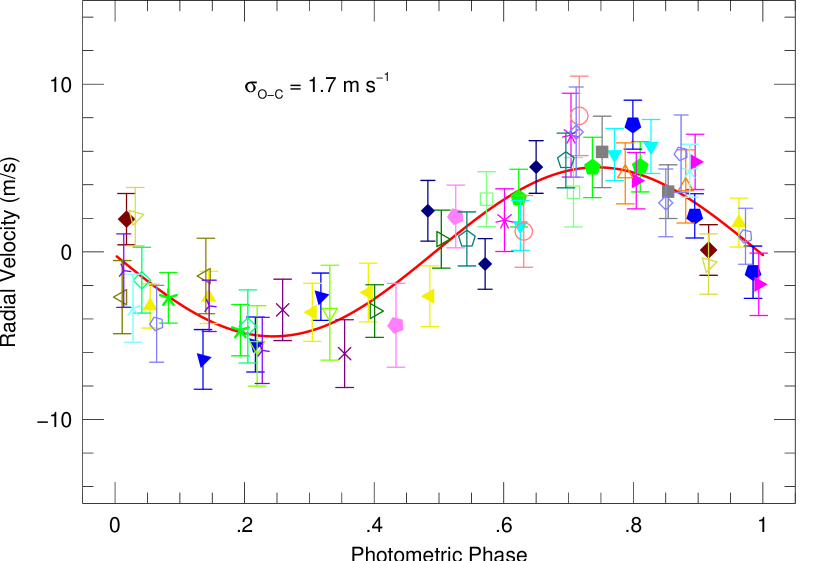
Figure 1: RV measurements for CoRoT-7b taken on the 27 nights listed in Table 1. On these nights multiple observations were made separated by 2–4 hours. Values are phased according the CoRoT transit phase. Different symbols represent measurements for different nights. The line represents the orbital solution.

Figure 1 shows the nightly RV measurements after removal of the nightly zero-point offsets and phased to the CoRoT transit ephemeris. Initially, the eccentricity was fixed at zero as was the ephemeris and orbital period. Allowing the phase to vary resulted in a value to within a phase of 0.01 to the CoRoT value. Varying the orbital eccentricity resulted in a small eccentricity ($e$ = 0.077) but with large errors ($\pm$ 0.11). The orbit is circular to within the error. The solution shown is for zero eccentricity and phase fixed to the transit phase. The resulting $K$-amplitude is 5.15 $\pm$ 0.95 m s^-1

When examining the data taken in a single night one clearly sees that the change in the RV almost always follows the orbit to within the measurement error. The rms scatter of the RV data about the orbital solution (line) is 1.68 m s^-1 which is in excellent agreement with the median RV internal error of 1.77 m s^-1. This figure alone argues that the contribution of activity jitter to this RV curve is negligible.

As a “sanity check” we performed a Scargle periodogram (Scargle 1982) on the calculated nightly offsets. This periodogram, shown in Figure 2, has its highest peak at a frequency of $\nu$ = 0.043 c d^-1, the known rotational frequency of the star. According to Scargle (1982) the probability that noise will produce this peak exactly at the rotational frequency is about 5$\times$10^-4. This was confirmed using a bootstrap randomization procedure. The RV data was randomly shuffled 200,000 times, keeping the times fixed and the maximum power in the random data periodogram was examined. Over the narrow frequency range 0.035–0.055 c d^-1 centered on the rotational frequency the false alarm probability that noise is causing the observed peak was 7$\times$10^-5. The derived nightly offsets thus have some relationship to a known phenomenon associated with the star (i.e. rotation). The RV amplitude of this peak is $\approx$ 10 m s^-1, consistent with the RV amplitude due to rotational modulation using the entire HARPS data set (Hatzes et al. 2010).

We performed Monte Carlo simulations to confirm the error on the $K$-amplitude, but more importantly to assess how well we could recover a known signal in the RV data. Given the relative sparse sampling of the sine-curve on each night there was some concern that when fitting a fixed period to the data the procedure may introduce variations with that period into the data due primarily to the freedom in varying the nightly offsets. A synthetic sine wave was generated with an amplitude of 5 m s^-1 and having the same period and phase of CoRoT-7b. The fake data was sampled in the same manner as the real data and random noise at a level of 2 m ^-1 was added. To mimic the activity signal random noise with an rms of 10 m s^-1 was added to the fake RVs for each night. The data was then processed in the same manner as the real data. One hundred such simulations yielded a mean amplitude of 5.00 $\pm$ 0.94 m s^-1 and in all cases the nightly “activity” signal was recovered to within the measurement error. The error in the $K$-amplitude from the simulations is entirely consistent with the measured value and suggests that the errors in the RV measurements are nearly Gaussian.

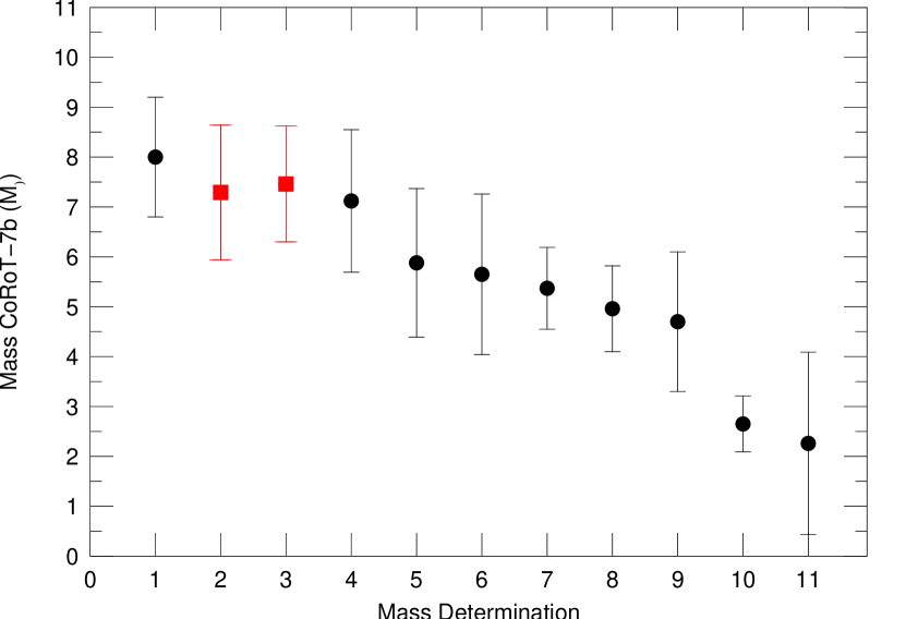
Figure 6: A comparison of the masses for CoRoT-7b that have been reported in the literature. The values on the abscissa correspond to numbers in Table 3. The squares mark the determinations in this work.

Figure 3 shows the RV measurements after they have been averaged in bins of approximately $\Delta\phi$ $\sim$ 0.05–0.1. The nightly zero-point offsets calculated using the unbinned data have been applied. We have plotted the abscissa and ordinate on the same scales used for the binned RV curve for Kepler-10b shown in Figure 6 of Batalha et al. (2010) so as to facilitate a direct comparison between the RV curves of these two superearths. This figure shows that in spite of an RV “jitter” of 10 m s^-1 for CoRoT-7, that with better temporal sampling and our simple treatment of the activity signal we can extract an RV curve that is much “cleaner” than for a quiet star such as Kepler-10b. We do have more free parameters in our fit - the nightly offsets due to activity - but by taking several measurements per night we can determine and correct for the RV jitter. This, of course, would be impossible with just a single RV measurement per night (or for a planet with a much longer orbital period). Calculating an orbit using the binned values and only 2 free parameters - the $K$-amplitude and a single zero-point velocity for all nights - results in an amplitude of $K$ = 5.21 $\pm$ 0.21 m s^-1. We believe this error to be artificially low because we are no longer fitting different nightly zero-points as we did with the unbinned data and these errors are correlated with the error in the $K$-amplitude. So, the error of $\sigma$ = $\pm$ 0.94 m s^-1 including the correlated errors of the nightly offsets is a more realistic assessment of the error in the $K$-amplitude. The rms scatter of the RV measurements about this orbital solution is 0.52 m s^-1.

3 Linear Model

Our Keplerian solution from the previous section established that the orbit of CoRoT-7b is circular and in phase with transit lightcurve. We can thus use a linear model of the form:

$$Acos(\omega t_{i})+Bsin(\omega t_{i})+C_{i},$$ (1)

where A and B determine the amplitude and phase of the sine function fitted to the RV periodic modulation, and $C_{i}\in\left\{\right.C_{1},...,C_{27}\left.\right\}$ are the different shifts for each of the 27 nights with multiple measurements (each $C_{i}$ is assumed to be constant for each night), $\omega=2\pi/P$ for a given period $P$ and $t_{i}$ is the time of each measurement. Presenting the model in the form of Equation (1) enabled us to apply a linear model to the data as the phase does not appear explicitly. The linear model assured a robustness of the best solution while The resulting radial velocity amplitude from the linear model was 5.25 $\pm$ 0.84 m s^-1. We shall use this value as our “best-fit” $K$-amplitude.

We also used the linear model as a “high pass filter” and applied it to the data using different frequencies. The periodogram of $1/\chi^{2}$ calculated with fits using frequencies in the range (0,2] days^-1 (Figure 4) shows a clear global maximum near Corot-7b’s period, which was found through photometry by Leger et al. (2009).

4 Derivative Fitting

The derivative of the RV curve should also be insensitive to the contribution of the activity and taking differences in the RV on a given night one should only detect changes due to orbital motion and the underlying (constant) activity signal removed. The fitting to the RV data done in the previous sections confirms that the orbit is circular and in phase with the CoRoT ephemeris. The RV curve can thus be described by the function: $V$ = $-Ksin(2\pi\phi)$ $+$ $C_{i}$, where $K$ is the RV amplitude, $\phi$ the orbital phase, $C_{i}$ is the nightly zero point, and the minus sign ensures that the RV curve has the proper phase with respect to the mid-transit time. Differentiating with respect to $\phi$ results in $dV$/d$\phi$ = $-2\pi K$cos($2\pi\phi$). So, a plot of the derivative (differences) of the RV values versus cos($\phi$) should have a linear relationship whose slope is proportional to the $K$-amplitude.

Figure 5 shows the normalized nightly RV derivatives ($dV/d\phi$/2$\pi$) as a function of $-$cos($\phi$). There is considerable scatter since we are dealing with differences, but there is a clear correlation. The correlation coefficient is $r$ = 0.59 with a probability of 6 $\times$ 10^-5 that the data is uncorrelated. A least squares fit to the derivatives yields a $K$-amplitude of 5.02 $\pm$ 1.25 m s^-1 a value entirely consistent with the previous approaches.

5 Contribution of the Activity Signal

Table 3 lists all the different $K$-amplitude determinations for CoRoT-7b from here and the literature. For Queloz et al. (2009) we include not only the adopted value, but the results from the individual methods for determining the RV amplitude. To ensure that the mass was determined in a consistent way using the same stellar and orbital parameters we recalculated these using the published $K$-amplitudes and the mass function (see below). These may result in slightly different values than quoted in the respective papers. These appear in the third column in the table and graphically in Figure 6. The number on the abscissa corresponds to that in the first column of the table. Our mass for CoRoT-7b agrees to within 1$\sigma$ to most other mass determinations. It is most discrepant (4$\sigma$) with the harmonic filtering without correction from Queloz et al. (2009), but the authors showed that the filtering process resulted in an unusually low value. The authors considered the adopted value of 4.96 $\pm$ 0.86 to be a more accurate determination.

Our mass value is clearly discrepant with the low value of 2.3 $\pm$ 1.8 M_⊕ (2.1$\sigma$) claimed by Pont et al. (2010), a mass determination largely responsible for casting doubt on the rocky nature of CoRoT-7b (Batalha et al. 2011). We believe the Pont et al. value to be artificially low, most likely due to their treatment of the activity. In modeling the RV and activity indicators they used 2-200 spots ($N$=12-20 could reproduce the light curves within the uncertainties). These spots were parameterized by a scale factor (no spot temperature was specified), a latitude, and a longitude. The spot evolution was characterized via a Gaussian with parameters of peak intensity, epoch, and lifetime. Differential was included, although values were not specified. A relatively large number of parameters and assumptions were used for fitting the observed quantities.

A better understanding of the nature of the 0.85-d RV variations of CoRoT-7b comes not from some ad hoc activity model, but rather from the RV curve itself. The striking feature about these curves (Figs. 1 and 3) is that they do not deviate from a circular orbit (i.e. pure sine curve) to within the errors using the period and phase of the photometric transit. We have 3 possibilities for the shape and amplitude of this sine curve: 1) it is due purely to a planet, 2) it is due purely to activity, or 3) it is due to a combination of both.

We can exclude points 2) and 3). For activity to contribute significantly to the RV curve it would have to have variations that would mimic the 0.85-d period and be perfectly in phase with the CoRoT-7b lightcurve ephemeris, otherwise we could not fit a circular orbit to the data. We could concoct a spot distribution that evolves with just the right time scales and phase with respect to the 0.85-d period, but that would be too ad hoc and lacking in a reasonable physical interpretation. The simplest and most logical way to produce a 0.85-d variation in the RV data, and one that has a stronger physical basis, is with the 1-day alias of $P_{rot}/4$ ($\nu$ = $\nu_{rot}$/4 + 1) which is close to the CoRoT-7b orbital frequency. Figure 8 of Hatzes et al. (2010) and the periodogram in Figure 4 demonstrate that the true period of 0.85-d is favored over the alias period and that it provides a better fit to the data. However, for the sake of argument let us assume that the RV curve in Figure 3 is indeed due to an alias of 4$\nu_{rot}$ rotational harmonic or at least makes a significant contribution to this curve. We argue that this cannot be the case for two strong reasons.

First, there is little evidence for the 4$\nu_{rot}$ actually being present in the activity indicators. Assuming that the Pont et al. $K$-amplitude of 1.6 m s^-1 is indeed correct, then the RV amplitude due to activity in Figure 3 amounts to 3.4 m s^-1. The RV amplitude associated with the rotational frequency is 8.7 m s^-1. This means that the third harmonic should have an amplitude $\approx$ 0.4 of the rotational peak. We find, however, weak evidence for significant power at 4$\nu_{rot}$. Figure 7 shows the discrete Fourier transform (DFT) amplitude spectra of the FWHM, the bisectors, and the Ca II emission. The vertical line marks the the location of $\nu_{rot}$/4 which is near the one-day alias of the orbital frequency of CoRoT-7b. Only the FWHM and Ca II show a bit of power near this rotational harmonic. The FWHM shows a ratio of the third harmonic to rotational frequency of only 0.2. Ca II does show a peak at the third harmonic with the proper amplitude ($\approx$ 0.4). However, the DFT of both the FWHM and bisector span are quite noisy with other peaks close to the third harmonic having a larger amplitude. Pont et al. (2010) argue that the FWHM can be used to reconstruct the brightness variations to 0.1% or better. If this is true, and since 4$\nu_{rot}$ has an amplitude 20% of the rotational peak, then the RV variations due to the third harmonic should be about 1.7 m s^-1, or comparable to the measurement error.

Second, and just as importantly, we would have to place very stringent constraints on the spot distribution and its evolution that are highly unlikely:

1. Physically, the only way to produce a strong presence of $P_{rot}$/4 in the RV rotational modulation is to have 4 spot groups equally spaced in longitude by 90^∘. Each spot group would produce its own sinusoidal variation and all four RV curves from the individual spot groups would add together to contribute to the observed 0.85-d RV variations (in this case, the one day alias of $P_{rot}$/4.)

2. For activity to reproduce the CoRoT transit phase and to be able to add or subtract to the RV curve in the proper phase, one spot group must be located at transit phase zero. Otherwise the activity signal would introduce significant distortions to the RV curve.

3. To produce the symmetrical RV curve in Figure 3 and with little scatter all four spot groups must have comparable filling factors, otherwise the envelope of RV curves from the individual spot groups would introduce significant “jitter” and the observed scatter of the RV data would exceed the measurement errors. For example, this is seen in the RV curve for Kepler-10 where the assumed RV jitter dominates the internal measurement error in spite of this star being “quiet” in terms of activity. (Batalha et al. 2011). Here the resulting binned RV curve is more distorted and “noisier” compared to that of CoRoT-7. This filling factor can be estimated using the expression of Hatzes (2006) or Saar & Donahue (1996). To produce a spot-induced RV amplitude of 5 m s^-1 requires a spot filling factor for each group of about 0.3 %. The difference in spot filling factor (areal coverage) can be estimated from the rms scatter about the orbital solution. For the RV curves from the different spot groups to produce variations less than the rms scatter of $\sigma$ = 1.68 m s^-1, they must have the same filling factors to within 70%. Using the binned RV values in order to minimize the measurement error of $\approx$ 2 m s^-1 then the differences in amplitudes between the RV curves of the four spot groups should be less than $\sigma$ = 0.5 m s^-1. In this case the spot filling factors for all spot groups must be the same to within about 10%.

4. A symmetrical RV curve also implies that the spot evolution over the span of the measurements for all four spot groups must be small. The RV measurements span more than 3.5 rotation periods and as noted by Pont et al. (2010): “no feature is reproduced unchanged after one rotation period, and the light curve becomes unrecognizable after merely 2-3 periods.” Having four spot groups that evolve very little over 3.5 rotation periods contradicts what we see in the light curve of CoRoT-7b.

So, either we have a star with a superearth planet (similar to Kepler-10b - see below), or we have a star with an extremely remarkable spot distribution. We thus conclude that the 0.85-d RV modulation seen in Figure 1 and Figure 3 is due almost entirely to the reflex motion induced by a planet.

We also see no evidence for any short term (i.e during the night) systematic errors in the RV data (possible long term errors are removed by subtracting the nightly mean). The error in each phase bin is just $\sigma_{RMS}$/$\sqrt{N}$ where $N$ are the number of points in each bin used for averaging. If the HARPS RV errors are estimated well, then this bin error should equal the mean RV error of the binned points divided by $\sqrt{N}$. The last two columns in Table 2 compares these two values (signified by $\sigma_{obs}$, $\sigma_{cal}$). The two values are consistent and the larger value was used as the error bar in Figure 3. We see no obvious evidence for short term systematic errors in the HARPS data. This is also in agreement with RV planet search programs conducted with HARPS. There are several dozen cases where the RV measurements of stars are in the same signal-to-noise regime as CoRoT-7 and these show a residual scatter in the range of 1.5–3.5 m s^-1 (Naef et al. 2010; Lo Curto et al. 2010; Moutou et al. 2011), comparable to what we see in CoRoT-7.

Taking all the arguments into account, the most reasonable, and most logical explanation for the 0.85-d RV variations of CoRoT-7 is that these are due entirely to the transiting planet, CoRoT-7b. Furthermore, the significance of this detection is at the 15$\sigma$ level.

6 The Bisector and FWHM Variations

Queloz et al. (2009) used a method similar to that of this paper to study the possible variations of the cross correlation function bisector possibly induced by the radial velocities variations due to the CoRoT-7b signal. For each of the observing nights with two or three measurements per night, they corrected the radial velocities from their average during the night over the two or three measurements. They did the same correction on the bisector span by their nightly average. These “differential” bisector spans and radial velocities can show short-period variations, on a time scale of about 5 hours which is the typical longest time offset between data in night with multiple observations. This represents 25% of the CoRoT-7b orbit.

The nightly variations of the bisector span as a function of the nightly variations of the radial velocities are plotted in Figure 8. It shows peak-to-peak variations on the order of 20 m s^-1 for the bisector spans and 10 m s^-1 for the radial velocities. The larger dispersion of the bisectors agrees with their error bars that are two times larger than those for the radial velocities. The bisectors show a hint for correlation with the radial velocities. With the hypothesis of a linear correlation, the data show a positive slope of $0.45\pm 0.22$ that is plotted in Figure 8 . The Spearman’s rank test indicates a 2$\sigma$ deviation from the null correlation hypothesis. A bootstrap with 30 000 pools mixing radial velocity and bisectors shows a slope distribution centered on zero, with only 1.9% probability to find a slope of $0.45$ or larger. It also shows a 2.1% probability to find by chance a deviation from the null correlation hypothesis greater than 2$\sigma$ with the Spearman’s test.

Thus, the data show a 2$\sigma$ detection of a positive correlation between the differential bisector spans and radial velocities, on a night-per-night basis. Such correlation could be the signature of blend scenario (e.g. Santos et al. 2002), where a star in the background of the main target hosts a deep transit which seems shallower as it is diluted by the constant, brighter flux of the main target. However, blend simulations presented by Queloz et al. (2009) have shown that the slope the bisector versus the radial velocity should be steeper than 2 in all cases, whereas $0.45\pm 0.22$ is found here. Thus the possible correlation between bisector spans and radial velocities apparently cannot be explained with a blend scenario. In addition, such blend scenario would have to imply that the background star hosts a deep transiting companion while the main star, by chance, hosts at least one planet (CoRoT-7c) as detected in radial velocities. A planetary system is more likely with the two companions orbiting the same stars.

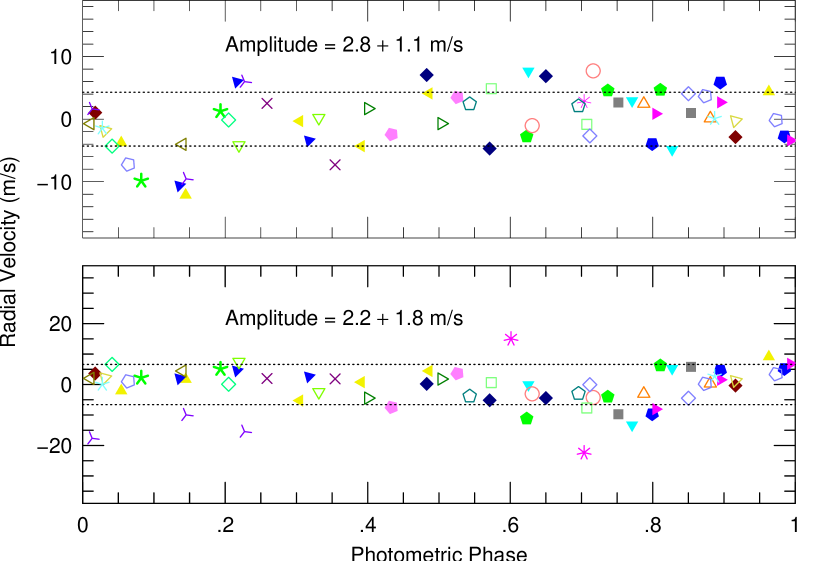
Figure 9: (Top) The residual bisector variations resulting from performing the same analysis as done on the RV data and phased to the photometric period. The dashed horizontal lines represent the $\pm 1\sigma$ calculated for the data in the phase interval 0.15–1.0. (Bottom) The residual FWHM resulting from performing the same analysis as done on the RV data phased to the photometric period.

To investigate further any possible bisector variations, the exact same analysis that was applied to the RV data was also applied to the bisector data. Namely, the nightly data was treated as independent data sets and a sine wave was fit to the data keeping the period fixed at 0.85 days and allowing the nightly means to float. The top of the Figure 9 shows the residual bisector variations after subtracting the calculated nightly mean and phased to the CoRoT-7b period. There is no compelling evidence for sinusoidal variations. A sine fit to the data yields an amplitude of 2.8 $\pm$ 1.1 m s^-1. The only hint of variability is driven by a cluster of only four points at phase $\approx$ 0.1. Eliminating these points in a much lower amplitude of 1.6 $\pm$ 0.9 m s^-1. Most of the bisector span data between phases 0.2–1.0 have an rms scatter of $\pm$1$\sigma$ as shown by the dashed lines. For now any possible bisector correlation or variations remain unexplained, but one should keep in mind that these variations with the present data set do not seem to be significant. Even though there are often large nightly variations, these are all within the rms scatter of about 4.5 m s^-1. (Compared to the $\approx$ 10 m s^-1 rms scatter for the bisector variations of Kepler-10b, see Figure 7 of Batalaha et al. (2011).) This also argues against any possible variations being due to a blend scenario.

We also applied this method to the FWHM measurements. This is shown in the bottom panel of Figure 9 where we plot the FWHM residuals phased to the 0.85-d period. The amplitude of any variations is 3.8 $\pm$ 3.2 m s^-1. There is no strong evidence for variability in the FWHM with a 0.85-d period.

7 Discussion

The planet mass can be derived from the $K$-amplitude via the mass function, $f(m)$ which for circular orbits (the most likely case for CoRoT-7b) is:

$$f(m)={{(m_{p}sini)^{3}}\over{M_{star}^{2}}}={{K^{3}P}\over{2\pi G}}$$ (2)

where $P$ is the orbital period, $M_{star}$ the stellar mass, and $G$ the gravitational constant. Bruntt et al. (2010) derived a stellar mass of 0.91 $\pm$ 0.03 $M_{\odot}$ and Léger, Rouan, Schneider et al. (2009) derived an orbital inclination of $i$ = 80.1 $\pm$ 0.3 degrees. Using the appropriate stellar and orbital parameters for CoRoT-7b and solving Eq. 1 for $m_{p}$ results in $m_{p}$ ($M_{\oplus}$) = (1.416 $\pm$ 0.031)$K$ (m s^-1). Our best fit $K$-amplitude of 5.25 $\pm$ 0.84 m s^-1 (linear model) results in $m$ = 7.42 $\pm$ 1.21 M_⊕.

Given our derived planet mass we can now estimate the bulk density of the planet. Bruntt et al. (2010) give a planet radius of 1.58 $\pm$ 0.1 $R_{\odot}$. This results in a mean planet density of 10.4 $\pm$ 1.8 gm cm^-3.

The large density of CoRoT-7b has been reinforced by the discovery of a second transiting superearth, Kepler-10b (Batalha et al. 2011). Kepler-10b has a slightly smaller mass, $m$ = 4.56 $\pm$ 1.23 $M_{\oplus}$ and a smaller radius, $R$ = 1.416 $\pm$ 0.033. (For simplicity we have taken the mean of the $\pm$ error values given in Batalha et al. 2011). However, to within the errors CoRoT-7b and Kepler-10b have identical bulk densities: $\rho_{Kepler-10b}$ = 8.8 $\pm$ 2.5 gm cm^-3 compared to $\rho_{CoRoT-7b}$ = 10.4 $\pm$ 1.8 gm cm^-3.

A detailed discussion on the possible internal structure of CoRoT-7b and Kepler-10b is well beyond the scope of this paper. We can, however, compare the density and radius to terrestrial bodies in our own solar system as well as to simple models. The inner terrestrial planets, excluding Mercury, and the Moon show a tight linear correlation between logarithm of the density, $\rho$, and planet radius, $R_{P}$ (correlation coefficient, $r$ = 0.99976). The terrestrial planets as well as the moon are shown in Figure 10 along with CoRoT-7b and Kepler-10b. Also shown are three models for a “super-Moon”, Earth-like, and a “super-Mercury”. The Earth-like planet has a silicate mantle that is 67% by mass and an iron core that is 10% by mass. A moon-like planet has a 100% silicate mantle (MgO and SiO₂) and no core. The Mercury-like planet has an iron core that is 63% of the mass and a silicate mantle 37% of the planet mass.

The nominal values of CoRoT-7b and Kepler-10b place these above the Earth-like planets and close to Mercury that is iron enriched. However, within the errors both of these exoplanets have a density and mass consistent with either an Earth-like planet or a super-Mercury. Whether CoRoT-7b and Kepler-10b have an internal structure similar to Mercury or the Earth requires reducing the error on the density. For CoRoT-7b equal contributions to the error come from the planet mass (19%) and radius (6%, but contributing as $R^{3}$ in the density). Kepler-10b benefits from a better measurement of the $R_{p}$ (due to the astroseismic determination of the stellar parameters), but the planet mass is known to within 26%, a bit worse than for CoRoT-7b. A substantial improvement in the mass of Kepler-10b can be realized by a reduction in the $K$-amplitude error. The RV measurements for Kepler-10b show an rms scatter about the orbit that is a factor of 2 larger than the internal errors. This is most likely due to the RV jitter of activity (Batalha et al. 2011). This activity jitter is estimated to be about 2 m s^-1, or 50% of the planet $K$-amplitude. So, in order to get a better mass determination for Kepler-10b one would have to correct for the activity signal, even for such a quiet star. Since Kepler-10b has a long rotational period ($P_{rot}$ = 50-100 d) the stellar activity jitter could be reduced by taking several measurements of Kepler-10 throughout the night when the star is well-placed in the sky and employing the procedure we used on CoRoT-7b. Unfortunately, the Kepler-10b RV measurements had only two nights where multiple measurements were taken.

In light of the discovery of Kepler-10b, the properties of CoRoT-7b may not be so extraordinary. It is remarkable that so quickly after the start of the space missions CoRoT and Kepler two transiting rocky planets with comparable (and possibly new) properties have been discovered. This bodes well for the detection of more of such objects.

In the case of CoRoT-7b and Kepler-10b, the two host stars are also very similar with each having about the same radius, mass, and $T_{eff}$. The largest difference is in the level of activity which is significantly lower in the case of Kepler-10. This is explained by Kepler-10 also being much older than CoRoT-7, about 8 $\pm$ 0.26 Gyr (as derived by asteroseismology). CoRoT-7 has an estimated age of 1.2–2.3 Gyr (Léger, Rouan, Schneider et al. 2009). The stars also differ somewhat in metalicity $[Fe/H]$ = +0.13 for CoRoT-7b (Bruntt et al. 2010) and $[Fe/H]$ = $-$0.1 for Kepler 10b (Batalha et al. 2011). Another similarity between the two systems is that of the very remarkable orbital period – 0.85d – for CoRoT-7b, which was unprecedented for such a low mass planet, is now mirrored in Kepler-10b with a period of 0.84d.

It should be noted here that if the mass of the exoplanet Kepler-9d (which is also orbiting a G-type star) is found to be close to the currently determined upper limit (7 M_⊕, Holman et al 2010), this body also would belong to the same type of planet. This is not the case for the small planets recently discovered around the star Kepler-11 (Lissauer et al. 2011), which if their masses are confirmed belong to a type with very much lower densities ($\approx$ 0.8–2 gm cm^-3), so there appears to be a wide range of properties of superearth exo-planets. Figure 10 hints that in terms of structure, CoRoT-7b and Kepler-10b may be more like Mercury than the other terrestrial planets. Clearly, more transiting superearths must be found - and with excellent mass and radius determinations - before we know if CoRoT-7b and Kepler-10b just represent a part of the “continuum” of low mass planets, or whether they are special even among short-period superearths.

Not surprisingly, the first confirmed superearths found by both CoRoT and Kepler are among the brightest stars in their respective samples. Because they are relatively bright it was possible to get the requisite precise RVs needed to confirm the nature of the transiting object. There are undoubtedly more CoRoT-7b-like planets to be found in the CoRoT and Kepler samples. Unfortunately, these are most likely among the fainter stars of the sample for which the RV determination of the mass is challenging. Clearly, to make significant progress in the understanding of the CoRoT-7b-type planets it is essential to find such objects around relatively bright stars for which characterization studies are easier. Unfortunately, the requisite precise photometry can only be conducted from space. This only emphasizes the need for such proposed space missions as PLAnetary Transits and Oscillations (PLATO, see Catala (2009)) and the Transiting Exolanet Survey Satellite (TESS, see Ricker et al. 2009) whose goals are to find transiting terrestrial planets among the brightest stars. In the case of PLATO, stellar parameters will be determined precisely using astroseismology which translates into more accurate planetary parameters. We will thus be able to determine if the “CoRoT-7b-like” planets are indeed more like Mercury than the Earth in terms of their internal structure.

Acknowledgments

The German CoRoT Team (Thüringer Landessternwarte and University of Cologne) acknowledges the support of grants 50OW0204, 50OW603, and 50QM1004 from the Deutsches Zentrum für Luft- und Raumfahrt e.V. (DLR). TM and GN acknowledge the support of the Israel Science Foundation (grant No. 655/07).

Figure 2: (top) The Scargle periodogram of the nightly offsets that were determined in the orbit fitting. The peak corresponds to the stellar rotational frequency of 0.043 c d^-1. (bottom) The Scargle periodogram of the offset residuals after removing the contribution of the dominant peak.

Figure 3: The phased RV measurements binned by units of $\Delta\phi$ $\approx$ 0.1. The line represents the same orbital solution as Figure 1. The rms scatter of the data values about the fit is 0.52 m s^-1

Figure 4: Periodogram of 1/$\chi^{2}$ versus frequency calculated using the linear model.

Figure 5: The normalize derivative, ($dV$/$d\phi$)/$2\pi$) calculated from successive RV measurements plotted versus the negative of the cosine of the orbital phase. The data have a correlation coefficient of $r$ = 0.59 and with the probability of 6 $\times$ 10^-5 that they are uncorrelated. The slope corresponds to an RV amplitude of $K$ = 5.02 $\pm$ 1.26 m s^-1.

Figure 7: The amplitude spectrum of the FWHM (top), bisectors (middle), and Ca II emission (bottom) calculate using the discrete Fourier transform. The vertical dashed line marks the location of the 4$\nu_{rot}$ which is the one-day alias of the orbital frequency of CoRoT-7b.

Figure 8: Bisector spans as a function of radial velocities (nightly variations). For each observing night, both bisector spans and radial velocities are corrected for the average value of the night. The typical error bars on each point are plotted in the bottom-right. There is a 2-$\sigma$ hint for the detection of a correlation between the bisector spans and the radial velocities. The linear correlation has a slope of $0.45\pm 0.22$ that is shown on the plot.

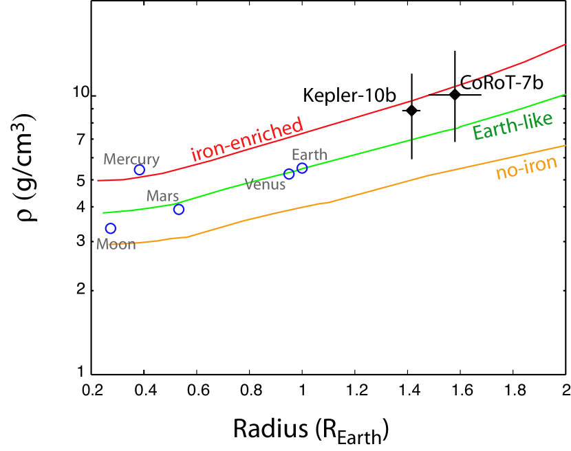
Figure 10: Density-Radius relationships for three types of rocky compositions. Earth-like: 67% by mass of silicate mantle with 10% iron by mol [(0.9MgO, 0.1Fe)+SiO₂] + 33% by mass of iron core. No-iron: 100% silicate mantle [MgO + SiO₂ mantle]. Iron-enriched: 37% silicate mantle (with 0% of iron by mol) + 63% iron core.

Table 1: Journal of Observations

Start	$N_{obs}$	$\Delta T$	$\Delta\phi$	$\Delta V_{C7c,d}$
		(hours)		(m s-1   )
2454799.7770	2	2.10	0.10	$-$0.33
2454800.9461	2	2.09	0.10	0.05
2454801.7530	2	2.08	0.10	0.76
2454802.7484	2	2.27	0.11	$-$0.45
2454803.7526	2	1.95	0.09	$-$0.95
2454804.7554	2	1.75	0.09	$-$0.07
2454805.7775	2	1.75	0.09	$-0.35$
2454806.7647	2	1.91	0.09	$-$0.42
2454807.7281	2	2.36	0.12	$-$0.18
2454847.5968	3	3.84	0.19	$-$1.63
2454848.6008	3	3.80	0.19	$-$0.78
2454849.5940	3	3.72	0.18	0.76
2454850.5951	3	3.72	0.18	$-$0.52
2454851.5927	3	3.72	0.18	1.19
2454852.7986	3	3.42	0.17	$-$0.17
2454853.5740	3	4.13	0.20	2.00
2454854.5802	3	3.88	0.19	$-$0.27
2454865.5978	2	2.83	0.14	0.01
2454867.5604	2	2.30	0.11	0.17
2454868.5918	2	2.30	0.11	0.32
2454869.6002	2	2.11	0.10	$-0.63$
2454870.6013	2	2.75	0.13	$-0.07$
2454872.5647	3	3.91	0.19	$-$1.43
2454873.5375	3	4.38	0.21	0.96
2454879.6002	2	3.35	0.16	1.33
2454882.5256	2	3.11	0.15	1.16
2454884.5265	2	2.87	0.12	$-$1.43

Table 2: Binned RV values

$\phi$	RV	$N_{obs}$	$\sigma_{obs}$	$\sigma_{cal}$
	(m s-1)		(m s-1)	(m s-1)
0.00	0.01	7	0.70	0.68
0.05	$-$2.03	6	0.93	0.80
0.14	$-$3.65	4	1.06	0.93
0.22	$-$4.89	6	0.37	0.80
0.36	$-$3.53	7	0.46	0.75
0.56	1.22	11	0.52	0.53
0.71	5.61	8	0.51	0.74
0.80	5.72	6	0.50	0.65
0.88	2.88	9	0.76	0.60

Table 3: Mass Determinations for CoRoT-7b

$N$	K-amplitude	Mass	Method	Reference
	(m s-1)	(M⊕)
1	5.70 $\pm$ 0.80	8.0 $\pm$ 1.20	High Pass Filtering	Ferraz-Melo (2011)
2	5.15 $\pm$ 0.95	7.29 $\pm$ 1.35	Model independent	This work
3	5.27 $\pm$ 0.81	7.46 $\pm$ 1.16	Linear model	This work
4	5.04 $\pm$ 1.09	7.12 $\pm$ 1.43	Offset fitting	Hatzes et al. (2010)
5	4.16 $\pm$ 1.00	5.88 $\pm$ 1.49	Pre-whitening	Queloz et al. (2009)
6	4.00 $\pm$ 1.60	5.65 $\pm$ 1.61	Harmonic Filtering	Boisse et al. (2011)
7	3.80 $\pm$ 0.80	5.37 $\pm$ 0.82	Harmonic Filtering w/correction	Queloz et al. (2009)
8	3.50 $\pm$ 0.60	4.96 $\pm$ 0.86	Adopted	Queloz et al. (2009)
9	3.33 $\pm$ 0.80	4.70 $\pm$ 1.40	Pre-whitening w/correction	Queloz et al. (2009)
10	1.90 $\pm$ 0.40	2.65 $\pm$ 0.56	Harmonic Filtering	Queloz et al. (2009)
11	1.60 $\pm$ 1.30	2.26 $\pm$ 1.83	Activity Modeling	Pont et al. (2010)

References

- Alonso et al. (2008) Alonso, R., et al. 2008, A&A, 492, 21
- Batalha et al. (2011) Batalha, N. M., et al. 2011, ApJ, 729, 27
- Baglin et al. (2006) Baglin, A., Auvergne, M., Bosnard, L., Lam-Trong, T., Barge, P., Catala, C., Deleuil, M., Michel, E., Weiss, W. 2006, 36th COSPAR Scientific Assembly. Held 16 - 23 July 2006, in Beijing, China. Meeting abstract from the CDROM, #3749
- Boisse et al. (2011) Boisse, I., Bouchy, F., Hébrard, G., Bonafils, X., Santos, N. C., Vauclair, S. 2011, A&A, 528, A4
- Bruntt et al. (2010) Bruntt, H., Deleuil, M., Fridlund, M., Alonso, R., Bouchy, F., Hatzes, A., Mayor, M., Moutou, C., Queloz, D. 2010, A&A, 519, 51
- Catala (2009) Catala, C. 2009, CoAst, 158, 330
- Ferazz-Mello et al. (2011) Ferraz-Mello, S., Tadeu dos Santos, M., Beauge, C., Mitchchenko, T.A, Rodrigiguez, A. 2011, A&A, in press
- Foukal (1987) Foukal, P. 1987, JGR, 92, 801
- Jefferys et al. (1988) Jefferys, W., Fitzpatrick, J., McArthur, B. 1988, Celest. Mech. 41, 39
- Hatzes (2002) Hatzes, A. P. 2002, AN, 323, 392
- Hatzes et al. (2010) Hatzes, A. P., Dvorak, R., Wucther, G., Guterman, P., Hartman, M., Fridlund, M., Gandolfi, D., Guenther, E., Pätzold, M. 2010, A&A, 520, 93
- Holman et al. (2010) Holman, M.J., Fabrycky, D.C., Ragozzine, D. et al 2010, Science, 330, 51
- Léger et al. (2009) Léger, A., et al. 2009, A&A, 506, 287
- Lissauer et al. (2011) Lissauer, J. J., et al. 2011, Nature, 470, 53
- Lo Curto et al. (2010) Lo Curto, G. Mayor, M., Benz, W., Bouchy, F., Lovis, C., Moutou, C., Naef, D., Pepe, F., Queloz, D., Santos, N.C., Segransan, D., Udry, S. 2010, A&A, 512A, 48L
- Naef et al. (2010) Naef, D., Mayor, M., Lo Curto, G., et al. 2010, 523, 15.
- Mayor et al. (2003) Mayor, M., Pepe, F., Queloz, D., et al. 2003, The Messenger, 114, 20
- Moutou et al. (2011) Moutou C., Mayor, M., Lo Curto, G., et al. 2011, A&A, 527, 63
- Queloz et al. (2009) Queloz, D., Bouchy, F., Moutou, C., et al. 2009, A&A, 506, 303
- Pont et al. (2006) Pont, F., Zucker, S., & Queloz, D. 2006, MNRAS, 373, 231
- Ricker et al. (2009) Ricker, G. et al. 2009, BAAS, 41, 193
- Saar & Donahue (1997) Saar, S. H., Donahue, R. A. 1997, ApJ, 485, 319
- Santos et al. (2002) Santos, N. et al. 2002. A&A, 392, 215
- Scargle (1982) Scargle, J.D., 1982, ApJ, 263, 835.
- Torres et al. (2011) Torres, G., Fressin, F., Batalha, N.M. et al., 2011, ApJ, 727, 24
- Valencia (2011) Valencia, D., 2011, in Detection and Dynamics of Transiting Exoplanets, eds. F. Bouchy, R. D az, C. Moutou, EPJ Web of Conferences, Volume 11, id.03001