How unusual are the Shapley Supercluster and the Sloan Great Wall?

Abstract

We show that extreme value statistics are useful for studying the largest structures in the Universe by using them to assess the significance of two of the most dramatic structures in the local Universe – the Shapley supercluster and the Sloan Great Wall. If we assume that the Shapley concentration (volume $\approx 1.2\times 10^{5}h^{-3}$Mpc³) evolved from an overdense region in the initial Gaussian fluctuation field, with currently popular choices for the background cosmological model and the shape and amplitude $\sigma_{8}$ of the initial power spectrum, we estimate that the total mass of the system is within 20 percent of $1.8\times 10^{16}h^{-1}\,M_{\odot}$. Extreme value statistics show that the existence of this massive concentration is not unexpected if the initial fluctuation field was Gaussian, provided there are no other similar objects within a sphere of radius $200h^{-1}$Mpc centred on our Galaxy. However, a similar analysis of the Sloan Great Wall, a more distant ($z\sim 0.08$) and extended concentration of structures (volume $\approx 7.2\times 10^{5}h^{-3}$Mpc³) suggests that it is more unusual. We estimate its total mass to be within 20 percent of $1.2\times 10^{17}h^{-1}M_{\odot}$ and we find that even if it is the densest such object of its volume within $z=0.2$, its existence is difficult to reconcile with the assumption of Gaussian initial conditions if $\sigma_{8}$ was less than 0.9. This tension can be alleviated if this structure is the densest within the Hubble volume. Finally, we show how extreme value statistics can be used to address the question of how likely it is that an object like the Shapley Supercluster exists in the same volume which contains the Sloan Great Wall, finding, again, that Shapley is not particularly unusual. Since it is straightforward to incorporate other models of the initial fluctuation field into our formalism, we expect our approach will allow observations of the largest structures – clusters, superclusters and voids – to provide relevant constraints on the nature of the primordial fluctuation field.

1 Introduction

Since its discovery (Shapley, 1930) the Shapley Supercluster has been the object of considerable interest because it potentially contributes significantly to the velocity field in the local Universe (e.g. Scaramella et al., 1989; Raychaudhury et al., 1991) and because the existence of extremely massive objects such as Shapley constrains the amplitude of the initial fluctuation field, and possibly the hypothesis that this field was Gaussian.

Recent studies suggest that the Shapley Supercluster contains a few times $10^{16}h^{-1}\,M_{\odot}$, is overdense by a factor of order 2, and is receding from us at about 15,000 km s^-1. These conclusions are based on studies of the motions of galaxies (Quintana et al., 2000; Reisenegger et al., 2000; Proust et al., 2006; Ragone et al., 2006) and estimates of the masses of X-ray clusters in this region (Reiprich et al., 2002; de Filippis et al., 2005). In addition, the fact that this region is over-abundant in rich clusters also allows an estimate of its mass (Muñoz & Loeb, 2008), not all of which may actually be bound to the system (Dünner et al., 2007; Araya-Melo et al., 2008). Whereas the other methods are observationally grounded, the mass estimate from this last method (i.e. from the over-abundance of rich clusters) follows from the assumption that the initial fluctuation field was Gaussian. Here, we refine this estimate of the total mass of Shapley and compare it with the answer to the question: What is the probability distribution of the mass of the most massive object, having the volume of Shapley, if it formed from Gaussian initial conditions? We use extreme value statistics to address this question. Although we do not explore this here, we note that our methods are easily extended to incorporate non-Gaussian initial conditions.

Section 2 summarizes a number of properties of the Shapley supercluster. Sections 3 and 4 describe our methods based on the excursion set approach and extreme value statistics, and what they imply for objects like Shapley, for which accurate estimates of the masses of the constituent clusters are available. Section 5 shows how to extend these approaches to study the Sloan Great Wall (Gott et al., 2005), for which accurate mass estimates of the components are not available. This requires combining a halo model (e.g., Cooray & Sheth, 2002) analysis of the galaxy population with a catalog of groups identified in this distribution. For the SDSS, we use the clustering and group analyses of Zehavi et al. (2005) and Berlind et al. (2006), respectively.

A final section summarizes our results, shows how extreme value statistics can be used to answer the question of how unusual it is that an object like the Shapley Supercluster exists in the same volume which contains the Sloan Great Wall, and discusses how our methods allow observations of the largest structures – clusters, superclusters and voids – to place interesting constraints on the nature of the initial fluctuation field. Where necessary we assume a flat $\Lambda$CDM model with $(\Omega_{0},\Omega_{b},h,\sigma_{8})=(0.27,0.046,0.72,0.8)$, but we also explore other choices of $\sigma_{8}$.

2 The Shapley Supercluster

The largest redshift survey which includes the Shapley supercluster suggests that it contains 8632 galaxies (Proust et al., 2006). These have been grouped into 122 systems of galaxies with 4 or more members (Ragone et al., 2006). We run a percolation algorithm on this catalog to identify the largest supercluster in this region. To do so, we neglect the peculiar velocity of the clusters: i.e., each cluster is assigned coordinates $x_{1}=r\cos\delta\cos\alpha$, $x_{2}=r\cos\delta\sin\alpha$ and $x_{3}=r\sin\delta$, where $(\alpha,\delta)$ are its celestial coordinates and $r=cz/H_{0}$. Figure 1 shows the pie diagram of these systems. Solid dots show the 40 systems belonging to the Shapley Supercluster when we use a linking length of $8h^{-1}$ Mpc. According to the virial masses computed by Ragone et al., 15 of these 40 clusters have masses larger than $10^{14}h^{-1}$ M_⊙. Summing the masses of these 40 clusters yields $5.42\times 10^{15}h^{-1}$ M_⊙. The total mass is expected to be considerably larger than this, because lower mass groups and galaxies are expected to contribute significantly to the total. Ragone et al. (2006) use mock catalogs, based on the VLS simulation of Yoshida et al. (2001), to account for this missing mass, and conclude that the total mass of Shapley is likely to be about $1.6\times 10^{16}h^{-1}M_{\odot}$.

Figure 1: Systems of galaxies of the (Ragone et al., 2006) sample in redshift space. Solid dots are the clusters belonging to the Shapley supecluster according to a percolation analysis with percolation length $8h^{-1}$ Mpc.

To quantify the shape of the Shapley supercluster, we compute the eigenvalues of the inertia tensor

$$I_{ij}={\sum_{k}m_{k}x_{ki}x_{kj}\over\sum_{k}m_{k}}\quad{\rm where}\quad i,j=1,2,3$$ (1)

where $m_{k}$ is the mass of each cluster, the coordinates $x$ are centered on A3558, and the sum is only over the cluster members. We find the three eigenvalues $8.30$, $5.48$, and $2.73h^{-1}$ Mpc. If we neglect the fact that the 40 cluster members have masses in the range $[0.008,6.717]\times 10^{14}h^{-1}$ M_⊙, and set $m_{k}=1$ for all $k$’s, the eigenvalues of the tensor of inertia are $7.69$, $6.02$, and $3.42h^{-1}$ Mpc; i.e., they are not substantially different from the previous values.

As a check, we have also applied our percolation analysis to an X-ray survey of this region, which shows 41 extended sources (de Filippis et al., 2005). A link length of $8h^{-1}$ Mpc links 8 clusters, and returns a total mass in X-ray clusters of $1.65\times 10^{15}h^{-1}$ M_⊙, where we estimated the mass of each cluster as follows:

$${M_{200}\over h_{50}^{-1}M_{\odot}}=\left(L_{\rm bol}\over 10^{A+40}h_{50}^{-2}{\rm erg}\;{\rm s}^{-1}\right)^{1/\alpha}$$ (2)

where $A=-22.1\pm 1.3$ and $\alpha=1.807\pm 0.084$ (Reiprich et al., 2002). With this recipe, only 5 out of the 8 members have masses larger than $10^{14}h^{-1}$ M_⊙. It is reassuring that these numbers are smaller than those of Ragone et al. (2006), because this sample of X-ray clusters with known redshifts is clearly incomplete (de Filippis et al., 2005). Therefore, in what follows, we use the cluster catalogue from Ragone et al. (2006), rather than from the X-ray data.

3 The excursion set approach

The previous section suggests that the total mass of the Shapley supercluster is at least $5\times 10^{15}h^{-1}M_{\odot}$. In this section, we make a rather different estimate of the total mass. According to Ragone et al. (2006), the inner $31h^{-1}$Mpc of Shapley centered on A3558 contains 58 galaxy systems: 19 of these have mass greater than $10^{14}h^{-1}M_{\odot}$. For such high masses, it is reasonable to equate each cluster with a single halo. Integrating the halo mass function (Sheth & Tormen, 1999) from this lower limit to infinity shows that the expected number in randomly placed spheres of this radius is only $2.67$. This number depends on $\sigma_{8}$: reducing $\sigma_{8}$ to 0.7 changes the expected count to 1.77; increasing to 0.9 makes the count 3.5. Neither of these numbers is close to that observed.

However, if Shapley is an overdense region, then the relevant comparison is not with the expected counts in a region of average density, but one which is overdense (Muñoz & Loeb, 2008). In theories of structure formation from Gaussian initial conditions, massive halos are expected to be more abundant in dense regions, and the mix of halos is expected to also be different. In dense regions, the halo mass function is expected to be top-heavy (Frenk et al., 1988; Mo & White, 1996; Sheth & Tormen, 2002), so this is an immediate signal that Shapley must be overdense in dark matter (Muñoz & Loeb, 2008). Measurements in the SDSS indicate that the halo mass function in regions which are overdense in galaxies is indeed top-heavy (Skibba et al., 2006; Abbas & Sheth, 2007), so it is interesting to ask if this effect is sufficient to explain the existence of a region like Shapley.

Figure 2: Expected number of clusters with masses greater than $10^{14}h^{-1}M_{\odot}$ as a function of the total mass of the supercluster. The expected number increases as $\sigma_{8}$ increases.

To make this estimate, we will make the crude assumption that Shapley is spherical, despite the fact that it is not, as we have shown in the previous section. However, by considering the most massive 19 clusters within a distance of $31h^{-1}$Mpc from A3558, rather than the system identified with the percolation analysis, we expect to make this assumption more reasonable. We will return to the issue of triaxiality in the final Discussion section.

Let $\bar{N}_{\delta}$ denote the mean number of halos with mass above threshold in a region which has volume $V$ and contains mass $M$ (so the mass overdensity is $1+\delta=M/\bar{\rho}V$):

$$\bar{N}_{\delta}=\int_{M_{\rm min}}^{M}{\rm d}m\,N(m,\delta_{c}|M,V).$$ (3)

This number increases as $M$ increases; the precise dependence can be computed following arguments in Sheth & Tormen (2002), which build on the work of Mo & White (1996), and are within the framework of the excursion set approach (Lacey & Cole, 1993; Bond et al., 1991). This approach requires an estimate of the relation between the overdensity in linear theory, $\delta_{\rm L}$ and the actual nonlinear overdensity $1+\delta$. We use the spherical model to do this:

$$1+\delta\approx\left(1-\frac{\delta_{\rm L}}{\delta_{\rm sc}}\right)^{-\delta_{\rm sc}},$$ (4)

where $\delta_{\rm sc}\approx 1.675$.

Let $p(M|V)$ denote the probability that a randomly placed cell of size $V$ contains mass $M$. If we assume that halo counts in cells of mass $M$ follow a Poisson distribution with mean $\bar{N}_{\delta}$ (see Sheth & Lemson, 1999, for why this is only accurate for large cells), then the probability that a cell of size $V$, in which there are $N$ clusters, contains mass $M$ is

$$p(M|N,V)=\frac{p(N|M,V)\,p(M|V)}{p(N|V)},$$ (5)

where

$$p(N|V)\equiv\int dM\,p(N|M,V)\,p(M|V),$$ (6)

and the Poisson assumption means

$$p(N|M,V)\equiv\frac{\bar{N}_{\delta}^{N}}{N!}\,\exp(-\bar{N}_{\delta}).$$ (7)

To proceed, we require a model for the probability $p(M|V)$ that a randomly placed cell of size $V$ contains mass $M$. Now, $p(M|V)$ can be estimated using the same excursion set framework as is used in the calculation of $\bar{N}_{\delta}$ (Sheth, 1998). Alternatively, on large scales, it could also be estimated using perturbation theory (Bernardeau et al., 2002). On these large scales, these two approaches are in good agreement: the shape of $p(M|V)$ which results is reasonably well approximated by a Lognormal (Lam & Sheth, 2008):

$$p(M|V)\,{\rm d}M\approx\frac{\exp(-y^{2}/2\sigma_{\rm L}^{2})}{\sigma_{\rm L}\,\sqrt{2\pi}}\,\frac{{\rm d}M}{M},$$ (8)

where $y=\ln(1+\delta)+\sigma^{2}_{\rm L}/2$, and $\sigma_{\rm L}^{2}$ is the variance in linear theory on scale $V$. For $\sigma_{8}=(0.7,0.8,0.9)$ and $V=(4\pi/3)31^{3}h^{-3}$Mpc³ our linear power spectrum yields $\sigma_{\rm L}=(0.23,0.26,0.29)$.

Figure 2 shows how $\bar{N}_{\delta}$, computed following Sheth & Tormen (2002), increases with total mass $M$ for our three choices of $\sigma_{8}$. This, in equation (5), allows us to constrain the expected values of $M$. The solid curve in Figure 3 shows $p(M|N,V)$ when $\sigma_{8}=0.8$. Figure 4 shows $p(M|N,V)$ for $\sigma_{8}=0.7$ (top) and $\sigma_{8}=0.9$ (bottom). In effect, these are estimates of the total mass, and hence overdensity, of Shapley. Notice that these distributions shift slightly with $\sigma_{8}$. The sense of the trend is easily understood: When $\sigma_{8}$ is small then massive halos are rare, so the environment must be that much more extreme to produce the observed number of clusters. At the peak values $\log(M/h^{-1}M_{\odot})=(16.28,16.26,16.25)$ the associated overdensities are $(1+\delta)=(2.07,1.99,1.93)$ so the linear theory overdensities are $\delta_{\rm L}=(0.60,0.56,0.54)$, making $(\delta_{\rm L}/\sigma_{\rm L})=(2.60,2.15,1.86)$. These indicate that Shapley is not particularly unusual. We argue in Section 4.1 that to estimate the initial ‘peak height’, it may be more appropriate to use $\sigma_{\rm L}(M)$ rather than $\sigma_{\rm L}(\bar{\rho}V)$. This yields higher values: $\delta_{\rm L}/\sigma_{\rm L}=(3.35,2.75,2.33)$. All these results are summarized in Table 1. It is remarkable that our analytic estimate of the total mass is so similar to that derived by Ragone et al. (2006) using mock catalogs: for $\sigma_{8}=0.9$ (the value in their mocks), our estimate is only 10% larger than theirs.

Upon evaluating an integral that is very similar to the one which defines $\bar{N}_{\delta}$, the excursion set approach also yields estimates of the typical mass fractions in such clusters. If we use $f_{\delta}$ to denote this fraction, then

$$\bar{f}_{\delta}=\int_{M_{\rm min}}^{M}{\rm d}m\,N(m,\delta_{c}|M,V)\,(m/M).$$ (9)

At the peak values shown in the Figures, $\bar{f}_{\delta}=$ (0.14, 0.18, 0.22) for $\sigma_{8}=(0.7,0.8,0.9)$. Since the total observed mass in these 19 clusters is $5.27\times 10^{15}h^{-1}M_{\odot}$, these mass fractions suggest total Shapley masses of $\log(M/h^{-1}M_{\odot})=(16.57,16.47,16.38)$. These values are larger than the peak values from the excursion set approach, because the expression above assumes that the observed number of clusters is equal to $\bar{N}_{\delta}$, whereas it is actually larger by a factor of $(1.7,1.6,1.5)$. Increasing $\bar{f}_{\delta}$ by these factors reduces the estimated total Shapley mass to $\log(M/h^{-1}M_{\odot})=(16.34,16.26,16.20)$. These values are in excellent agreement with our estimate above, which was based on the fact that 19 massive clusters were observed, but no other information about their masses was used, though the agreement is best for $\sigma_{8}=0.8$.

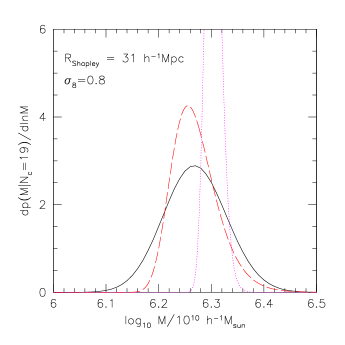
Figure 3: Comparison of the excursion set estimate of the mass of the Shapley supercluster (solid) with the expected mass of the densest of $N=(200/31)^{3}$ and the sixth densest of $N=(575/31)^{3}$ randomly placed cells having the same volume as Shapley (dashed and dotted), when $\sigma_{8}=0.8$.

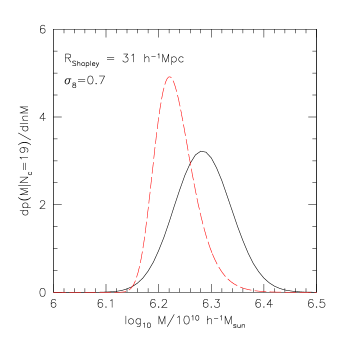
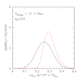
Figure 4: Dependence of the estimated mass of the Shapley supercluster (solid) and of the densest of $(200/31)^{3}$ randomly placed Shapley-sized cells (dashed) on $\sigma_{8}$.

4 Extreme value statistics

It is interesting to compare the mass estimates derived above with the mass associated with the densest of $N$ randomly placed cells, where $N$ is the ratio of Shapley’s volume to that in which it was found. If the masses agree, then this would suggest that although Shapley is extreme, it is not unusually so. Note that, despite the similarity, this is a different question from the one which is more often asked: Is the region containing Shapley the densest of its size in the entire sphere centered on our galaxy which contains Shapley?

Given a total survey volume, the mass of the densest of $N$ cells placed randomly in this volume (i.e., large compared to the cells) – which we will estimate below – is certainly smaller than the mass associated with the question that is more usually asked. This is because one might think of this densest region as a particularly carefully placed cell. In particular, one would have to throw a large number of cells (compared to $N$) before one lands in just the right position to find this densest region. We discuss the difference between these two extreme value estimates in Section 4.3. Of course, both require an assumption about the volume within which Shapley was found. We will assume that this is a sphere with radius $200h^{-1}$Mpc, and will discuss how our results depend on this choice shortly (e.g. following equation 12).

If $P_{1}(<M|V)$ denotes the probability that the most massive of the $N=(200/31)^{3}$ regions of volume $V=V_{\rm Shapley}$ that are within $200h^{-1}$Mpc is less massive than $M$, then $P_{1}(<M|V)$ must equal the probability that each of the $N\approx 270$ cells is less massive than $M$. Thus

$$P_{1}(<M|V)=\int_{0}^{M}{\rm d}M\,p_{1}(M|V)\approx p(<M|V)^{N},$$ (10)

and, by taking the derivative,

$$p_{1}(M|V)\approx N\,p(M|V)\,p(<M|V)^{N-1}.$$ (11)

Appendix A discusses this approximation further.

Before we use this expression, notice that if $M_{1/2}$ denotes the median value of the expected mass, i.e., that at which $P_{1}(<M_{1/2}|V)=1/2$, then

$$-\frac{\ln(2)}{N}\approx\ln[1-p(>M_{1/2}|V)]\approx-p(>M_{1/2}|V),$$ (12)

where we have assumed that $p(>M|V)\ll 1$ in the tail of the distribution. This shows that the mass returned by our approach is approximately the same as that given by setting $Np(>M|V)=1$ (because $\ln 2$ is of order unity), which makes intuitive sense. It also illustrates that the mass estimate depends on $N$: If the large $M$ tail falls exponentially, then $M_{1/2}\propto\ln(N/\ln(2))$. I.e., the expected mass increases approximately as $\ln(N)$, so the dependence on $N$, and hence on our assumption that $V$ is the comoving volume within $200h^{-1}$Mpc, is weak.

This means that one can devise a test which asks if the survey volume which is required to make a certain mass object the densest of its type does indeed contain only one such object. Alternatively, if the survey volume is known but the mass is not, then the assumption that the object is the most massive actually yields an estimate of its mass. We will show shortly that Shapley passes either of these tests for currently acceptable values of $\sigma_{8}$.

Finally, we note that the mass estimate can be rather precise. If we use $M_{0.84}$ to denote the value of the mass below which $84\%$ of the probability lies, namely the value at $+1\sigma$, then, for an exponentially falling distribution in $M$, $M_{0.84}\propto\ln(N/\ln(1/0.84))$, so

$$\frac{M_{0.84}}{M_{1/2}}=1+\frac{\ln(\ln(2)/\ln(1/0.84))}{\ln(N/\ln(2))}=1+\frac{1.38}{\ln(N/\ln(2))}\;.$$ (13)

For $N=1000$ the fractional error on $M_{1/2}$ is 0.19, and it decreases as $\ln(N)$ increases.

4.1 Extremes in the initial conditions

To illustrate the approach, suppose that the pdf associated with scale $V$ is a Gaussian with variance $\sigma_{\rm L}$. Then the extreme-value mass and survey volume are related, through equation (12), by

$${\rm erfc}\left(\frac{\delta_{L}}{\sigma_{\rm L}\sqrt{2}}\right)=\frac{2\ln(2)}{V_{\rm Survey}/V},$$ (14)

where $\delta_{\rm L}$ is related to $M/V$ by equation (4). The previous section argued that, if $\sigma_{8}=0.8$, then, for an object like Shapley, $\sigma_{\rm L}=0.26$ and $\delta_{\rm L}/\sigma_{\rm L}=2.15$. These values in equation (14) imply $V_{\rm Survey}/V\approx 44$. Since this is substantially smaller than 270, there should be at least 6 other Shapley-like objects within $200h^{-1}$Mpc of us. This is unlikely. Alternatively, requiring $V_{\rm Survey}/V=270$ means $\delta_{\rm L}/\sigma_{\rm L}=2.8$. For $\sigma_{\rm L}=0.26$, the associated nonlinear overdensity is $1+\delta=2.6$ making the estimated mass $10^{16.42}h^{-1}M_{\odot}$. This is about 0.18 dex larger than that from the excursion set approach, indicating that although Shapley is a rich concentration, it is not more extreme than one would expect on the basis of random statistics. Therefore, it would not be unexpected to find an even more extreme object of its volume in the local universe.

One can improve on these estimates by noting that if one is using the linear pdf, then the appropriate smoothing scale is not $V$ but the associated initial scale $M/\bar{\rho}$, and $\sigma_{\rm L}$ should also be computed on the scale $M/\bar{\rho}$ rather than $V$ (e.g., Lam & Sheth, 2008). Since $\sigma_{\rm L}$ is smaller than before, $\delta_{\rm L}/\sigma_{\rm L}$ will be larger, and we now require

$${\rm erfc}\left(\frac{\delta_{L}}{\sigma_{\rm L}(M)\sqrt{2}}\right)=\frac{2\ln(2)}{V_{\rm Survey}/V(1+\delta)}.$$ (15)

The result is that $V_{\rm Survey}/V\approx 232(1+\delta)=464$. Thus, Shapley is consistent with being the densest of $(200/31)^{3}$ cells, so we should not be surprised if we find another comparable or even more massive object in a survey that is only slightly deeper. Alternatively, if we set $V_{\rm Survey}/V=270$, then equation (15) requires Shapley’s mass to be $10^{16.245}h^{-1}M_{\odot}$, which is in good agreement with the excursion set analysis.

			Excursion	Extremes
$\sigma_{8}$	$\delta_{\rm L}/\sigma_{\rm L}$	$\delta_{\rm L}/\sigma_{\rm L}(M)$	$\log_{10}Mh/M_{\odot}$	$\log_{10}Mh/M_{\odot}$
0.7	2.60	3.35	16.28	16.22
0.8	2.15	2.75	16.26	16.25
0.9	1.86	2.33	16.25	16.29

Table 1: Estimated initial fluctuation height and mass of the Shapley supercluster. The values listed in columns 2 and 3 show that this large concentration of galaxies is not unlikely.

4.2 Extremes in the nonlinear field

It is interesting to contrast this treatment, which uses extreme value statistics of the initial pdf, with an analysis based on the nonlinear pdf. In the previous section, we used the fact that the Lognormal distribution (equation 8) is a reasonably accurate model. In this case, the distribution of $\ln(M)$ is Gaussian, so the previous analysis goes through except that now

$${\rm erfc}\left(\frac{\ln(M/\bar{\rho}V)+\sigma_{\rm L}^{2}/2}{\sigma_{\rm L}\sqrt{2}}\right)=\frac{2\ln(2)}{V_{\rm Survey}/V}.$$ (16)

The associated estimate for $V_{\rm Survey}/V=N$ given the excursion set mass of $10^{16.26}h^{-1}M_{\odot}$ and $\sigma_{\rm L}=0.26$ is 270. The small differences compared to the previous estimates can be understood as deriving from the fact that the term in brackets in the erfc above effectively makes Shapley a fluctuation of height $2.79$ (for $\sigma_{8}=0.8$).

In fact, the distribution of the expected mass is skewed. Hence, to provide a more direct comparison with the mass estimates from the previous section, which we also expressed as distributions, the dashed curves in Figures 3 and 4 show equation (11) for the same Lognormal distributions of $p(M|V)$ that we used in the excursion set calculation. The overlap between the solid and dashed curves is remarkable, given how very different these two methods are. E.g., for this calculation, the most probable mass $M$ decreases as $\sigma_{8}$ decreases (dashed curves in Figure 4), because small values of $\sigma_{8}$ mean that large deviations from the mean value are rarer; this trend is opposite to that for the excursion set approach, where small values of $\sigma_{8}$ mean massive halos are rarer, so the total mass $M$ from which to obtain the observed number of massive halos must be larger. So it is interesting that the match between these two approaches is slightly better for $\sigma_{8}=0.8$ than for the other two cases. When $\sigma_{8}=0.8$, then Shapley is consistent with being the most massive of a random set of regions of volume $V_{\rm Shapley}$ in the local Universe; if $\sigma_{8}=0.9$, then Shapley lies at the low-end of the expected extreme-mass distribution; if $\sigma_{8}=0.7$, then it lies at the high-mass end.

These curves show that, if it is the most extreme object within $200h^{-1}$Mpc, then the existence of Shapley is easily accomodated in models with high $\sigma_{8}$; even $\sigma_{8}=0.7$ is not problematic. On the other hand, if $\sigma_{8}=0.9$, then, we will not have to increase the survey volume much before we see another object that is more extreme than Shapley. However, if $\sigma_{8}=0.7$, then Shapley should be the most extreme object even in a volume that is larger by a factor of 2. It happens that there is indeed a very large structure in the volume which lies just beyond Shapley. The next section studies this structure in more detail.

But before we do, it is worth noting that our extreme value mass estimate is rather precise: the widths of the dashed curves in Figures 3 and 4 are typically less than 0.1 dex. While this level of precision may be surprising, we note that its origin is understood: setting $N=270$ in equation (13) yields a fractional uncertainty of 0.23, which corresponds to $0.1$ dex.

4.3 Peaks and extremes

So far, the extremes we have been considering are associated with the statistics of randomly placed cells. However, we noted that we are often more interested in ascertaining whether or not a particular object is an extreme outlier – since we have determined the location and size of the object a priori, treating it as a randomly placed cell is no longer appropriate. At least for sufficiently overdense extremes, there is a relatively straightforward way to account for this difference. This is because sufficiently overdense objects in the nonlinear density field typically correspond to large fluctuations in the initial field: i.e., $\nu_{\rm L}\equiv\delta_{\rm L}/\sigma_{\rm L}\gg 1$. For such objects, it should be a good approximation to assume they formed from high peaks in the initial field (also see discussion in Colombi et al. 2011). The expected number density of peaks above some $\nu_{t}$ (which we would like to estimate) is related to the probability that a randomly placed cell lies above this same threshold as follows. Typically, one can move the cell which defined the peak around a little bit without significantly changing the height of the fluctuation in it. If we think of this as defining a volume around each peak, then

$$P(\geq\nu_{\rm t})=\frac{{\rm erfc}(\nu_{\rm t}/\sqrt{2})}{2}={\rm vol}(\geq\nu_{\rm t})\,n_{\rm pk}(\geq\nu_{\rm t}).$$ (17)

If the peak was associated with smoothing scale $R_{M}$, then this volume satisfies

$${\rm vol}(>\nu_{\rm t})=\frac{(2\pi)^{3/2}R_{M}^{3}}{(\gamma R_{M}/R_{*})^{3}\,(\nu_{\rm t}^{3}-\nu_{\rm t})}\qquad{\rm as}\ \nu_{\rm t}\to\infty$$ (18)

Bardeen et al. (1986). This shows that the volume scales approximately as $\nu_{\rm t}^{-3}$, with prefactors that can be understood as follows. The volume of a Gaussian smoothing filter is $(2\pi)^{3/2}\,R_{f}^{3}$, so the numerator is the moral equivalent of what we have been calling the volume of the randomly placed cell in the initial conditions: $V(1+\delta)$. This means that

$$\frac{V_{\rm Survey}}{V(1+\delta)}\,P(\geq\nu_{\rm t})=\frac{n_{\rm pk}(\geq\nu_{\rm t})\,V_{\rm Survey}}{(\gamma R_{M}/R_{*})^{3}\,(\nu_{\rm t}^{3}-\nu_{\rm t})}\,.$$ (19)

If we now replace the requirement that $[V_{\rm Survey}/V(1+\delta)]\,P(\geq\nu_{\rm t})=1$ with the requirement that $n_{\rm pk}(\geq\nu_{\rm t})\,V_{\rm Survey}=1$ (see equation 12 and below), then this means that we now want

$$\frac{V_{\rm Survey}}{V(1+\delta)}\,P(\geq\nu_{\rm t})=\frac{1}{(\gamma R_{M}/R_{*})^{3}\,(\nu_{\rm t}^{3}-\nu_{\rm t})}.$$ (20)

Comparison with equation (15) shows that the required $V_{\rm Survey}$ is reduced by a factor proportional to $(\nu_{\rm t}^{3}-\nu_{\rm t})$. For scale-free spectra, $(\gamma R_{M}/R_{*})^{3}=[(n+3)/6]^{3/2}$, and, for the large smoothing scales of interest here ($\sim 30h^{-1}$Mpc), we can think of a $\Lambda$CDM model as having $n$ between $0$ and $-1$. This makes the required $V_{\rm Survey}$ smaller by a factor of approximately $2^{3/2}/\nu_{\rm t}^{3}$ or $3^{3/2}/\nu_{\rm t}^{3}$. Alternatively, if $V_{\rm Survey}/V$ is fixed, then the associated value of $\nu_{\rm t}$, and hence the associated mass estimate, will be larger than before. Although the relation between the value from the peaks calculation and that for random cells depends on $\nu_{\rm t}$, at $\nu_{\rm t}\sim 5$ (the high peaks of most interest here), the peaks calculation returns approximately 1 plus the value from the random cells calculation.

Figure 5: Dependence of the extreme value estimate of the height of the highest peak on the ratio of survey to peak volumes.

We can combine extreme value and peak statistics to make a slightly more detailed statement. Namely, for a given ratio of survey to peak volume, what is the expected distribution of the height of the highest peak? The same logic which led to equations (10) and (11) implies that

$$p_{\rm 1pk}(\nu)\approx n_{\rm pk}(\nu)\,V_{\rm Survey}\,{\rm exp}[-n_{\rm pk}(>\nu)V_{\rm Survey}].$$ (21)

(The Appendix discusses how one might go beyond the Poisson/independent cells assumption.) Figure 5 shows this distribution for a number of choices of

$$N_{\rm eff}\equiv(\gamma R_{\rm pk}/R_{*})^{3}\,\frac{V_{\rm Survey}}{(2\pi)^{3/2}R_{\rm pk}^{3}}.$$ (22)

To make the plot, we have used the $\nu\gg 1$ approximation (4.14) of Bardeen et al. (1986) rather than the full expression for $n_{\rm pk}(\nu)$, since we only expect this analysis to be valid for $\nu\gg 1$. But this does not affect the main point we wish to make: that the height of the highest peak is only a weak function of $N_{\rm eff}$. This is the analogue of the statement we made previously about the weak dependence of $M_{1/2}$ on $N$. The lesson is that very large survey volumes are required to reach large values of $\nu$.

Note in particular, that this analysis is only valid for $\nu$ larger than the one given by the excursion set analysis of Shapley, so we will not make numerical estimates of these effects here. However, in the next section, we will be interested in larger $\nu$, and this analysis will then be useful.

Figure 6: The Great Wall in the SDSS (filled circles), identified by a percolation analysis of the SDSS percolation group catalog (dots). Open circles show the additional members which are included if the percolation link length is increased from $8h^{-1}$Mpc to $12h^{-1}$Mpc.

5 The SDSS Great Wall

A dramatic structure at $z\sim 0.08$ is seen in the 2dF and SDSS galaxy surveys. Now known as the Sloan Great Wall (Gott et al., 2005), it is, like Shapley, a region containing an overabundance of rich clusters. We would like to perform a similar exercise to determine if it too can be easily accomodated in Gaussian theories. However, in this case, we do not yet have mass estimates of its members, and the appropriate lower limit in equation (3) is unknown. Therefore, we have extended our approach as follows.

5.1 Percolation estimates of Wall volume

We begin with the SDSS percolation catalog of groups in the SDSS (Berlind et al., 2006). This provides a list of about $4100$ groups having three or more members brighter than $M_{r}=-19.9$. We perform our own percolation analysis on this group catalog to identify the members of the Great Wall. The size of the Wall depends on the parameters of our percolation analysis; we have found that a link-length of $8h^{-1}$ Mpc returns a catalog that closely corresponds to the contiguous structure picked out by eye. This is approximately given by $0.07\leq z\leq 0.092$ and $0\leq{\rm dec}\leq 6$ if $185\leq{\rm ra}\leq 210$ and $0.07\leq z\leq 0.080$ and $0\leq{\rm dec}\leq 6$ if $166\leq{\rm ra}\leq 185$. The underlying group catalog and the Great Wall members identified by our analysis are shown as dots and filled circles in Figure 6. The Wall defined in this way contains 2180 galaxies in 335 groups. It has a volume of approximately $2.3\times 10^{5}h^{-3}$Mpc³, so its effective radius is about $38h^{-1}$Mpc; $\sigma_{\rm L}=0.212\,(\sigma_{8}/0.8)$ on this scale.

We note that the Wall appears to extend beyond the SDSS footprint towards negative declination. Because this cut reduces our estimates of both the number of group members and the total volume, neither our excursion set nor our extreme value analyses are strongly affected by this cut.

Our estimate of the total volume is determined from redshift-space quantities. For a structure as large as this, the redshift-space volume is smaller than the real-space volume. Figure 6 suggests that, along the line of sight, the structure varies from about 5000 km s^-1 to about 2000 km s^-1. If we assume that line-of-sight velocities are unlikely to exceed 1000 km s^-1, then the true structure may be larger in the redshift direction by a factor of between 1.2 and 1.5. Hence, we may have underestimated the true volume of the Wall by this same factor. In Section 5.3, we will show that our conclusions about whether or not the Wall is unexpected are not very sensitive to this uncertainty.

On the other hand, our choice of link-length makes the Wall significantly smaller in extent than claimed by Gott et al. Indeed, our estimate of the Wall’s volume makes it only $(38/31)^{3}=1.8$ times larger than Shapley. A link-length of about $12h^{-1}$Mpc is required to get something approaching their definition (open circles). In this case, the total volume is about $7.2\times 10^{5}h^{-3}$Mpc³ (effective radius $55h^{-1}$Mpc), $\sigma_{\rm L}=0.139\,(\sigma_{8}/0.8)$, and the structure contains 3663 galaxies in 645 groups. Again, varying the total volume by $\sim 30\%$ makes little difference to the nature of our conclusions below. More importantly, we will show that although our estimates of the mass in the Wall do depend strongly on the link-length used to define the Wall (the longer link-length yields a Wall with three times the volume, so one naively expects the mass to be about three times larger as well), our conclusions about how unusual the Wall is do not depend strongly on this choice.

5.2 A halo model-excursion set estimate of the Wall mass

A halo model analysis of the underlying galaxy catalog (i.e., SDSS galaxies with $M_{r}<-19.9$) suggests that only halos above $M_{\rm min}=10^{12}M_{\odot}$ host such galaxies. In halos of mass $m$ which host such galaxies, the probability of hosting $N_{s}$ additional galaxies (with $M_{r}<-19.9$) is given by a Poisson distribution with mean

$$\langle N_{s}|m\rangle=\left(\frac{m}{23\,M_{\rm min}}\right)^{1.16}$$ (23)

(Zehavi et al., 2005). To an excellent approximation, this relation between the galaxy population and halo mass is independent of environment (Abbas & Sheth, 2007). This is a key point, because it means that the relation above is expected to be as accurate for the halos in the Sloan Great Wall as elsewhere. Moreover, this assumption has also been shown to accurately reproduce the properties of the galaxies in the percolation group catalog we are using here (Skibba et al., 2007).

In the present context, the accuracy of the halo model decomposition, and of the Poisson distribution of $N_{s}$ in particular, means that we expect the fraction of halos of mass $m$ which host 3 or more galaxies to be

$$f_{3}(m)=1-{\rm e}^{-\langle N_{s}|m\rangle}(1+\langle N_{s}|m\rangle).$$ (24)

Similar expressions for $f_{n}(m)$ can be defined for arbitrary $n$. Hence, the expected number of halos containing $n$ or more galaxies brighter than $M_{r}=-19.9$ that are in cells of volume $V$ containing total mass $M$ is

$$\bar{N}_{\delta}=\int_{M_{\rm min}}^{M}{\rm d}m\,N(m,\delta_{c}|M,V)\,f_{n}(m),$$ (25)

where $M_{\rm min}=10^{12}h^{-1}M_{\odot}$ and $N(m,\delta_{c}|M,V)$ is the same quantity as before (c.f. equation 3), but with the new value of $V$. Indeed, the only significant difference from equation (3) is that we have now included a factor of $f_{n}(m)$ to account for the fact that only a fraction of halos of mass $m$ are expected to be in the group catalog. Note that this factor does not depend on $M$ or $V$, because the large scale environment does not affect equation (23).

With this expression for $\bar{N}_{\delta}$ in hand, we can now use equation (5) along with the observed number $N$ of groups having $n$ or more galaxies, and our estimate of the total volume $V$ of the Great Wall to estimate its mass $M$. For $\sigma_{8}=0.8$, the rms fluctuation on scale $V$ in linear theory is $\sigma_{\rm L}=0.142$. As before (equation 7), we assume a Poisson distribution for the number of groups, but now with mean given by equation (25). An important check on our approach is to perform this analysis for a range of values of $n$: the inferred mass distribution should not be sensitive to this choice. For $n=(3,4,5,6,7,8,9,10)$ the observed number of groups is $N_{\rm groups}=(335,199,132,96,75,68,60,49)$ when the link-length is $8h^{-1}$Mpc. For the longer link-length $12h^{-1}$Mpc, $N_{\rm groups}=(645,361,219,155,117,96,84,69)$.

The curves in the top panel of Figure 7 show a number of estimates of the mass of the Great Wall, when the link-length is $8h^{-1}$Mpc and $\sigma_{8}=0.8$. The dotted curve, which is shifted towards larger masses than any of the other curves is for $n=3$. This offset may be due to the difficulties associated with identifying small groups. For $n>5$, the distributions overlap: we have shown $n=6,7$ and 8. This is a nontrivial self-consistency test of our method. However, at $n>10$ (not shown) the distributions shift further towards smaller masses; it may be that here we are in the regime of small number statistics, where the number of groups contributing to the estimate has dropped below 50, so that Poisson errors on $N_{\rm group}$ are more than 10% of $N_{\rm group}$.

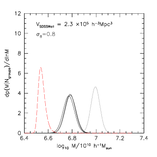
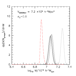
Figure 7: Comparison of the excursion set estimate of the mass of the Sloan Great Wall (solid) with the expected mass returned from the extreme value statistics approach (dashed) if $\sigma_{8}=0.8$. Top and bottom panels show results when the Wall and its members are defined using link-lengths of $8h^{-1}$Mpc and $12h^{-1}$Mpc, respectively. Different solid curves in each panel show the excursion set results for groups having more than $n=6,7$, and $8$ members; the dotted curve is for $n=3$. The excursion set mass estimate shifts to lower masses as $n$ increases, although it is quite stable around $n=7$; it is significantly larger than the estimate from extreme value statistics.

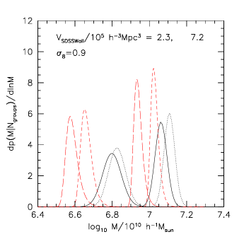
Figure 8: Similar to previous figure, but now $\sigma_{8}=0.9$. The left-most long dashed curve shows the extreme value result for the shorter ($8h^{-1}$Mpc) link-length, the short dashed curve just to the right of it shows the result of increasing $V_{\rm Wall}$ by 30%, to approximately account for $z$-space effects. The solid and dotted curves to the right of this curve show the corresponding excursion set estimates (we only show the $n=7$ result). The next set of long- and short-dashed, solid, and dotted curves show these same quantities when the Wall is defined by the longer ($12h^{-1}$Mpc) link-length.

These curves suggest that the total mass in the Wall is about $10^{16.77}h^{-1}M_{\odot}$, meaning that the structure is about 3.55 times denser than the background. This in equation (4) gives the associated linear theory density $\delta_{\rm L}$. In terms of the linear theory rms on this scale, we find $\delta_{\rm L}/\sigma_{\rm L}=4.2$. Using $\sigma_{\rm L}(M)$ instead makes this $6.6$. The overdensity in halos depends on $n$; it has 10 times the expected number of halos when $n=9$, but 9 times the expected mean number when $n=7$. This is consistent with the fact that dense regions are expected to be overabundant in massive halos, and increasing $n$ removes lower mass halos. The associated mass fraction in the observed groups (equation 9) varies from about 40% for $n=4$ to about 30% for $n=9$.

The corresponding results when the Wall is defined by the longer link-length are shown in the bottom panel. In this case, the total mass in the Wall is $M=10^{17.1}h^{-1}M_{\odot}$, so it is 2.25 times the background mass density, making $\delta_{\rm L}/\sigma_{\rm L}=4.6$; using $\sigma_{\rm L}(M)$ instead makes this $6.3$. The overdensity in halos is about 5, and the observed groups account for about 20 percent of the total mass. This smaller mass fraction is a direct consequence of defining the Wall as a looser structure.

5.3 Extreme value statistics

The dashed curves in the two panels show the estimate of the mass associated with the extreme value statistics argument of Section 4. This estimate requires as input the total survey volume, which we have set equal to the total comoving volume within $z=0.2$, making $V_{\rm Survey}/V_{\rm Wall}=3456$ and $1100$ for the two (short and long) linking lengths. In contrast to when we performed this analysis for the Shapley supercluster, the dashed curve now lies to the left of the solid curves: the excursion set estimates of the mass significantly exceed those expected based on extreme value statistics. This means that, if the excursion set estimates are reliable, then the existence of the Wall is difficult to reconcile with the standard model.

Increasing $\sigma_{8}$ alleviates the discrepancy slightly, as Figure 8 illustrates (solid and long-dashed curves). If $\sigma_{8}=0.9$ and $n=7$, then the excursion set analysis of the structure defined by the $8h^{-1}$Mpc link length estimates a mass overdensity of $3.7$, a halo overdensity of $7.7$, $\delta_{\rm L}/\sigma_{\rm L}=3.8$ and $\delta_{\rm L}/\sigma_{\rm L}(M)=6.2$. These numbers are $2.2$, $4$, $4.04$ and $5.5$ when the link length is $12h^{-1}$Mpc (Table 2). For either structure, these are significantly larger than the extreme value estimate of the expected mass of the densest object.

The second set of curves associated with each estimate (short-dashed and dotted lines) show the result of accounting crudely for redshift-space effects by increasing the Wall volume by 30%. To first order, increasing the volume increases all the mass estimates, but does not change the discrepancy between the extreme value and excursion set estimates. This is the basis for our claim earlier that accounting for $z$-space distortions does not change our conclusions. A more careful look shows that, the extreme value and excursion set mass estimates shift upwards by slightly different amounts: about 0.1 and 0.05 dex, respectively. As a result, although the peaks are still quite well-separated, the tails of the mass estimates overlap slightly more. This means that the tension between excursion set and extreme value masses is alleviated somewhat, particularly for the $12h^{-1}$Mpc link-length.

Thus, however we define it, the Wall is substantially more massive compared to the expected mass of the densest of $V_{\rm Survey}/V_{\rm Wall}$ randomly placed cells. This can be appreciated directly from the fact that the excursion set analyses returned estimates of $\delta_{\rm L}/\sigma_{\rm L}\approx 4$ for the Wall, compared to $\approx 2$ for Shapley (for $\sigma_{8}=0.8$), even though $V_{\rm Survey}/V_{\rm Wall}$ is not much larger than $(200/31)^{3}$.

It is interesting, therefore, to ask if its mass is also difficult to reconcile with the peaks model of Section 4.3, which attempts to account for the fact that the Wall is not just a randomly placed cell. In this case, an object with the mass and volume of the Wall would not be unusual only if it is the largest structure within a few times $10^{8}\,V_{\rm Wall}$; i.e., essentially within the Hubble volume. Expressed another way, if $\sigma_{8}=0.8$ then the expected mass of the most extreme peak within $z=0.2$ is $10^{16.57}$ or $10^{16.95}$ for our two definitions of the Wall. Although these are slightly larger than the randomly placed cells estimate, they are significantly smaller than the excursion set estimate.

						Excursion	Extremes
$V/10^{5}h^{-3}{\rm Mpc}^{3}$	$\sigma_{8}$	$\delta_{\rm L}/\sigma_{\rm L}$	$\delta_{\rm L}/\sigma_{\rm L}(M)$	$1+\delta_{M}$	$1+\delta_{n}$	$\log_{10}Mh/M_{\odot}$	$\log_{10}Mh/M_{\odot}$
2.3	0.8	4.2	6.6	3.55	9	16.77	16.54
2.3	0.9	3.8	6.2	3.70	8	16.80	16.57
7.2	0.8	4.6	6.3	2.25	5	17.07	16.91
7.2	0.9	4.04	5.5	2.20	4	17.07	16.94

Table 2: Estimated initial fluctuation height, mass overdensity, galaxy overdensity and mass of the SDSS Great Wall. The two upper rows refer to the $8h^{-1}$Mpc link length; the two lower rows to $12h^{-1}$Mpc.

6 Discussion and an extension

We discussed a number of methods for estimating the masses of extreme objects in the Universe, and applied them to two of the most dramatic objects in the local Universe: the Shapley supercluster and the Sloan Great Wall. We used a percolation analysis to define these systems, and illustrated how our results depended on the link-length ($8$ or $12h^{-1}$Mpc) used to define it.

In the case of Shapley, our estimate of the mass comes from combining estimates of the masses of its constituents with an excursion set analysis of the depedence of the halo mass function on the density of the local environment. Unfortunately, this was not possible in the case of the Wall, since mass estimates of its constituents are not available. In this case, we combined the excursion set analysis with a Halo-Model interpretation of its constituent groups, themselves identified from (optical) SDSS redshift survey data. Unfortunately, this method cannot currently be applied to Shapley, since it lies outside the SDSS footprint. This is also why we have not included results from the recent analyses of the Wall by Einasto et al. (2010, 2011) – but we hope to do so soon.

We compared these mass estimates with that expected for the densest object in an appropriately defined ‘local’ universe, and argued that the existence of Shapley is easily explained by currently popular models of structure formation (Figures 3 and 4); its mass ($1.82\times 10^{16}h^{-1}M_{\odot}$) is consistent with it being the most massive object of its volume ($1.25\times 10^{5}h^{-3}$Mpc³) within $200h^{-1}$Mpc.

On the other hand, the Sloan Great Wall (Figure 6) is difficult to explain, especially if the amplitude of the initial fluctuation field was at the low end of currently accepted values (Figures 7 and 8). Its mass $(5.9,12.6)\times 10^{16}h^{-1}M_{\odot}$ is larger than expected for the most massive object of its volume $(2.3,7.2)\times 10^{5}h^{-3}$Mpc³ within $z=0.2$ (where the two numbers are for defining the Wall using link-lengths of $8$ or $12h^{-1}$Mpc respectively). If $\sigma_{8}=0.8$, then insertion of the excursion set estimate of its mass in our extreme value statistics calculation suggests that it must be the densest object of its volume within the Hubble volume. An analysis which combines the excursion set estimate of the initial overdensity associated with the Wall, $\delta/\sigma\approx 6$, with the assumption that this fluctuation was the largest peak in the initial conditions, leads to a similar conclusion (Figure 5).

We are hesitant to make strong statements about whether this makes the Great Wall inconsistent with Gaussian initial conditions with acceptable values of $\sigma_{8}$, primarily because our current numbers are based on assuming the Wall is spherically symmetric when it clearly is not. For this reason, we are in the process of extending both our methods – the excursion set and extreme value statistics analyses – to account for this. Here we are aided by the fact that the Wall itself is not virialized. Hence, we can use the simple parametrization of triaxial collapse from Lam & Sheth (2008) to generalize equation (4) for the mapping between nonlinear and linear overdensity. This can then be used in our excursion set analysis. With this estimate of initial overdensity and shape in hand, we can modify our extreme value statistics calculation by replacing the number density of initial density of peaks of specified scale and height by adding the constraint that comes from specifying the shape (e.g., Bardeen et al., 1986). This is the subject of work in progress.

Our results suggest that the Sloan Great Wall is about 5 times the volume and about the same factor times the mass of the Shapley supercluster (we have used the larger mass and volume estimates of the Wall). So one might wonder if Shapley is about the sixth most extreme object of its volume within $z=0.2$. It is straightforward to extend our application of extreme value statistics to address this question. In particular, the same logic which leads to equation (11) implies that the expected distribution of the mass of the $n$th densest region is

$$p_{n}(M|V) \approx {N\choose n}\,n\,p(M|V)\,\Bigl{[}1-p(<M|V)\Bigr{]}^{n-1}$$ (26)

$$\qquad\qquad\times\quad p(<M|V)^{N-n}$$

(e.g. Gumbel, 1966). The dotted curve in Figure 3 shows this expression, evaluated with $n=6$, $N=6375$, and $\sigma_{\rm L}=0.24$. This shows that Shapley could easily be the sixth most massive object within $z=0.2$ if $\sigma_{8}=0.8$. Of course, it is trivial to extend this to our extreme value treatment of peaks: one simply replaces $p(<M|V)\to\exp(-n_{\rm pk}(>\nu)\,V_{\rm Survey})$. The Appendix discusses how to modify this approach to account for the clustering of peaks.

Similarly, one can write down expressions for the joint probability distribution of the masses of e.g., Shapley and the Great Wall, if we require one to be the $i$th and the other the $j$th most extreme object of its type (recall they may have different values of $\sigma_{\rm L}$) in the same survey volume – although we have not reproduced them here.

One of the surprises of these analyses is, perhaps, the precision of the mass estimates it returns: typically, these are of order 15%, both for the excursion set and the extreme value statistics approaches. Although we provided some analysis for why this is so (equation 13), it would have been nice to test our mass estimates by combining the motions of the clusters in these systems with an infall model. However, because the Shapley supercluster and the Sloan Great Wall are both far from round (e.g. Section 2), estimates based on the spherical collapse model are inappropriate. Therefore, we are currently in the process of developing an infall model based on the assumption of a triaxial collapse.

The precision of the mass estimates derives from the fact that the extreme fluctuations we are considering are from Gaussian random fields, in which extreme fluctuations are rare, so the distribution of events on the tail will be similar to one another. However, it is almost certain that, at least for the extreme value statistics calculation, this is more generic. This is because a large class of initial distributions have, as their limiting extreme value statistic, a double-exponential form (Fisher & Tippet, 1928; Gumbel, 1966). In the astrophysical context, this Fisher-Tippet or Gumbel distribution, and the study of extreme value statistics in general, has a long history in the study of the brightest galaxies in clusters (Scott, 1957; Bhavsar & Barrow, 1985). Our work suggests that extreme value statistics may continue to provide insight into the study of the largest structures in the Universe.

In particular, it would be interesting to use this approach to see if the sizes of the largest voids, or the masses of the most massive clusters or superclusters (e.g. Luparello et al. 2011; Schirmer et al. 2011; Yaryura et al. 2011), are consistent with the hypothesis that the initial fluctuation field was Gaussian. To use our approach for more generic initial conditions, one must know how the halo mass function depends on the large scale environment and one must have a model for the nonlinear probability distribution function. For non-Gaussian initial conditions of the local type, such models have recently become available (Lam & Sheth, 2009).

Appendix A On the approximation of independent cells when calculating extreme values of spatial statistics

The calculation of extreme value statistics reduces to one of writing the probability that, of $n$ draws from a distribution, none are above a certain value. This raises the question of whether or not the draws can be assumed to be independent picks. For the spatial statistics we are considering here, in which each cell represents a pick, and the total volume is the sum of the cells, the answer is clearly ‘no’ because there are correlations between the cells. On the other hand, since the correlations decrease with cell separation, most cells will only be strongly correlated with a few nearby cells. Moreover, since we will generally be interested in large cells, even nearby cells are likely to be only weakly correlated. So the assumption of independence, may in fact be quite good. The question is: Are extreme value statistics likely to be distorted by even these weak correlations? After all, the whole point of such stastistics is that they are sensitive to the tails of the distribution, and these are where (fractional) changes to the distribution will be largest. In what follows, we quantify this effect.

To proceed, we need an expression for the joint distribution of $n$-draws. We will first use a multivariate Gaussian to illustrate the argument, and then discuss possible generalizations. If $\delta_{i}$ denotes the value of the field at position $i$, then the multivariate Gaussian distribution is specified by the covariance matrix $C$, the elements of which are $C_{ij}=\langle\delta_{i}\delta_{j}\rangle$ (we are assuming $\langle\delta_{i}\rangle=0$ for all $i$). In our case, $C_{ij}$ will be a function of the separation $r$ between cells $i$ and $j$. Namely,

$$C_{ij} \equiv \frac{\sigma_{ij}^{2}(r)}{\sigma_{ii}(0)\sigma_{jj}(0)}\qquad{\rm where}$$ (27)

$$\sigma^{2}_{ij}(r) \equiv \int\frac{{\rm d}k}{k}\,\frac{k^{3}P(k)}{2\pi^{2}}\,W(kR_{i})W(kR_{j})\,\frac{\sin(kr)}{kr},$$

and we have allowed for the fact that the cells of interest at position $i$ may have a different size than those at position $j$. In the main text we were primarily interested in the case $R_{i}=R_{j}$. If the $R_{i}$ are large, and/or the separation between cells is large, then $C$ will be close to diagonal, so the $n$-point distribution will be well-approximated by the product of $n$ 1-point distribution functions. As a result,

$$\int_{-\infty}^{\delta_{c}}{\rm d}\delta_{1}\cdots\int_{-\infty}^{\delta_{c}}{\rm d}\delta_{n}\,p(\delta_{1},\cdots,\delta_{n})\approx\prod_{i}^{n}\int_{-\infty}^{\delta_{c}}{\rm d}\delta_{i}\,p(\delta_{i}).$$ (28)

This is the approximation used in equation (10) of the main text. The leading order correction to this can be obtained by writing this in terms of integrals above $\delta_{c}$, and then using previous results for high peaks or dense patches Bardeen et al. (1986); Jensen & Szalay (1986) to evaluate the result, which shows that the expression gets a correction factor which, to lowest order, depends on the two-point correlation function of regions above $\delta_{c}$.

In practice, the present day 1-point distribution function is no longer Gaussian. However, on large scales, it may be a good approximation to assume that there is a monotonic mapping between the nonlinear overdensity and the linear one. E.g., the main text assumes that this mapping is well approximated by a lognormal. If one assumes that this is also true of the $n$-point distribution function, then we have a fully specified model of the nonlinear $n$-point function, expressed in terms of the initial Gaussian covariance matrix. Now, the extreme value statistics care about the cumulative distribution: the monotonicity of the mapping means that the net effect of nonlinear evolution is simply to shift the threshold of the corresponding multivariate (linear theory) Gaussian. Once this shift has been applied, then the previous analysis of the Gaussian case goes through in its entirety. This justifies our use of equation (10), and also shows how it might be improved.

A.1 Including the clustering of extrema

Equation (21) in the main text follows from the assumption that peaks are uncorrelated, so the probability that there are no peaks in $V_{\rm survey}$ is given by the Poisson expression $\exp(-n_{\rm pk}V_{\rm Survey})$. This can be derived from equation (28), by taking the limit of infinite sampling (in which $n\to\infty$, so the typical spacing between the cells is no longer of order their size). Going beyond the Poisson model requires a calculation of the higher order correlation functions (White 1979). These are only known approximately (Appendix F in Bardeen et al. 1986). On large scales where these are small, the required replacement in equation (21) is

$$n_{\rm pk}(\geq\nu)V_{\rm Survey}\to n_{\rm pk}(\geq\nu)V_{\rm Survey}-[n_{\rm pk}(\geq\nu)V_{\rm Survey}]^{2}\frac{\bar{\xi}_{\rm pk}}{2},$$

where, for high peaks on large scales,

$$[n_{\rm pk}(\geq\nu)\,V_{\rm Survey}]^{2}\bar{\xi}_{\rm pk}\approx[n_{\rm pk}(\geq\nu)b_{\rm pk}(\geq\nu)V_{\rm Survey}]^{2}\bar{\xi}$$ (29)

$$\approx \left[N_{\rm eff}\,(\nu^{4}+\nu^{2}+2)\,\frac{\exp(-\nu^{2}/2)}{\sqrt{2\pi}}\right]^{2}\,\frac{\sigma_{0}^{2}(R_{\rm Survey})}{\sigma_{0}^{2}(R_{\rm pk})}.$$

Including this extra term affects the distributions shown in Figure 5 for $N_{\rm eff}<10^{3}$ or so (the peak shifts to slightly larger $\nu$) but matters little for larger $N_{\rm eff}$.

References

- Abbas & Sheth (2007) Abbas U., Sheth R. K., 2007, MNRAS, 378, 641
- Araya-Melo et al. (2008) Araya-Melo P. A., Reisenegger A., Meza A., van de Weygaert R., Dünner R., Quintana H., 2009, MNRAS, 399, 97
- Bardeen et al. (1986) Bardeen J. M., et al., 1986, ApJ, 304, 15
- Berlind et al. (2006) Berlind A., et al., 2006, ApJS, 167, 1
- Bernardeau et al. (2002) Bernardeau F., Colombi S., Gaztañaga E., Scoccimarro R., 2002, Phys. Rep. 367, 1
- Bhavsar & Barrow (1985) Bhavsar S. P., Barrow J. D., 1985, MNRAS, 213, 857
- Bond et al. (1991) Bond J. R., Cole S., Efstathiou G., Kaiser N., 1991, ApJ, 379, 440
- Colombi et al. (2011) Colombi S., Davis O., Devriendt J., Prunet S., Silk J., 2011, MNRAS, in press
- Cooray & Sheth (2002) Cooray A., Sheth R. K., 2002, Phys. Rep., 372, 1
- Davis et al. (2011) Davis O., Devriendt J., Colombi S., Silk J., Pichon C., 2011, MNRAS, in press
- de Filippis et al. (2005) de Filippis E., Schindler S., Erben T., 2005, A& A, 444, 387
- Dünner et al. (2007) Dünner R., Reisenegger A., Meza A., Araya P. A., Quintana H., 2007, MNRAS, 376, 1577
- Einasto et al. (2010) Einasto M., et al., 2010, A&A, 522, A92
- Einasto et al. (2011) Einasto M., et al., 2011, arXiv:1105.1632
- Frenk et al. (1988) Frenk C. S., White S. D. M., Davis M., Efstathiou G., 1988, ApJ, 327, 507
- Fisher & Tippet (1928) Fisher R. A., Tippet L. H. C., 1928, Proc. Camb. Phil. Soc., 24, 180
- Gott et al. (2005) Gott J. R. III, Juric M., Schlegel D., Hoyle F., Vogeley M., Tegmark M. Bahcall N., Brinkmann J., 2005, ApJ, 624, 463
- Gumbel (1966) Gumbel E. J., 1966, Statistics of Extremes, Columbia Univ. Press, New York
- Jensen & Szalay (1986) Jensen L. G., Szalay A. S., 1986, ApJ, 305, L5
- Lacey & Cole (1993) Lacey C., Cole S., 1993, MNRAS, 262, 267
- Lam & Sheth (2008) Lam T. Y., Sheth R. K., 2008, MNRAS, 386, 407
- Lam & Sheth (2009) Lam T. Y., Sheth R. K., 2009, MNRAS, 395, 1743
- Luparello et al. (2011) Luparello H. E., Lares M., Lambas D. G., Padilla N. D., 2011, MNRAS, submitted (arXiv:1101.1961)
- Mo & White (1996) Mo H. J., White S. D. M., 1996, MNRAS, 282, 347
- Muñoz & Loeb (2008) Muñoz J., Loeb A., 2008, MNRAS, 391, 1341
- Quintana et al. (2000) Quintana H., Carrasco E. R., Reisenegger A., 2000, AJ, 120, 511
- Proust et al. (2006) Proust D., Quintana H., Carrasco E. R., Reisenegger A., Slezak E., Muriel H., Dünner R., Sodré Jr. L., Drinkwater M. J., Parker Q. A., Ragone C. J., 2006, A& A, 447, 133
- Ragone et al. (2006) Ragone C. J., Muriel H., Proust D., Reisenegger A., Quintana H., 2006, A&A, 445, 819
- Raychaudhury et al. (1991) Raychaudhury S., Fabian A. C., Edge A. C., Jones C., Forman W., 1991, MNRAS, 248, 101
- Reisenegger et al. (2000) Reisenegger A., Quintana H., Carrasco E. R., Maze J., 2000, AJ, 120, 523
- Reiprich et al. (2002) Reiprich
- Scaramella et al. (1989) Scaramella R., Baiesi-Pillastrini G., Chincarini G., Vettolani G., Zamorani G., 1989, Nature, 338, 562
- Scott (1957) Scott E. L., 1957, AJ, 62, 248
- Schirmer et al. (2011) Schirmer M., Hildebrandt H., Kuijken K., Erben T., 2011, A&A, submitted (arXiv:1102.4617)
- Shapley (1930) Shapley H., Ames A., 1930, Harvard Coll. Obs. Bull., 880, 1
- Sheth (1998) Sheth R. K., 1998, MNRAS, 300, 1057
- Sheth & Lemson (1999) Sheth R. K., Lemson G., 1999, MNRAS, 304, 767
- Sheth & Tormen (1999) Sheth R. K., Tormen G., 1999, MNRAS, 308, 119
- Sheth, Mo & Tormen (2001) Sheth R. K., Mo H. J., Tormen G., 2001, MNRAS, 323, 1
- Sheth & Tormen (2002) Sheth R. K., Tormen G., 2002, MNRAS, 329, 61
- Sheth & van de Weygaert (2004) Sheth R. K., van de Weygaert R., 2004, MNRAS, 350, 517
- Skibba et al. (2006) Skibba R. A., Sheth R. K., Connolly A. J., Scranton R., 2006, MNRAS, 369, 68
- Skibba et al. (2007) Skibba R. A., Sheth R. K., Martino M. A., 2007, MNRAS, 382, 1940
- Skibba & Sheth (2009) Skibba R. A., Sheth R. K., 2009, MNRAS, 392, 1080
- Yaryura, Baugh, & Angulo (2011) Yaryura C. Y., Baugh C. M., Angulo R. E., 2011, MNRAS, 413, 1311
- Yoshida, Sheth, & Diaferio (2001) Yoshida N., Sheth R. K., Diaferio A., 2001, MNRAS, 328, 669
- Zehavi et al. (2005) Zehavi I., et al., 2005, ApJ, 630, 1