Earthquake networks based on similar activity patterns
Abstract
Earthquakes are a complex spatiotemporal phenomenon, the underlying mechanism for which is still not fully understood despite decades of research and analysis. We propose and develop a network approach to earthquake events. In this network, a node represents a spatial location while a link between two nodes represents similar activity patterns in the two different locations. The strength of a link is proportional to the strength of the cross-correlation in activities of two nodes joined by the link. We apply our network approach to a Japanese earthquake catalog spanning the 14-year period 1985-1998. We find strong links representing large correlations between patterns in locations separated by more than 1000 km, corroborating prior observations that earthquake interactions have no characteristic length scale. We find network characteristics not attributable to chance alone, including a large number of network links, high node assortativity, and strong stability over time.
I Introduction
Despite the underlying complexities of earthquake dynamics and their complex spatiotemporal behavior kagan1991 ; marsan2000 , celebrated statistical scaling laws have emerged, describing the number of events of a given magnitude (Gutenberg-Richter law) GR , the decaying rate of aftershocks after a main event (Omori law) omori ; utsu1961 ; utsu1995 , the magnitude difference between the main shock and its largest aftershock (Bath law) bath , as well as the fractal spatial occurrence of events knopoff ; turcotte ; okubo ; kirata . Recent work has shown that scaling recurrence times according to the above laws results in the distribution collapsing onto a single curve unify ; unify2 . However, while the fractal occurrence of earthquakes incorporates spatial dependence, it appears to embed isotropy in the form of radial symmetry, while the occurrence of real-world earthquakes is usually anisotropic bvalue .
To better characterize this anisotropic spatial dependence as it applies to such heterogeneous geography, network approaches have been recently applied to study earthquake catalogs AS3 ; AS2 ; AS4 ; AS1 ; davidsen2006 ; lofti2012 ; pasten ; pasten2 . These recent network approaches define links as being between successive events, events close in distance davidsen2006 , or being between events which have a relatively small probability of both occurring based on three of the above statistical scaling laws leastlikely . These methods define links between singular events. In contrast, we define links between locations based on long-term similarity of earthquake activity. While earlier approaches capture the dynamic nature of an earthquake network, they do not incorporate the characteristic properties of each particular location along the fault. Various studies have shown memory ; influence ; lennartz ; corral ; omori that the interval times between earthquake events for localized areas within a catalog have distributions not well described by a Poisson distribution sornette1997 , even within aftershock sequences corral . This demonstrates that each area not only has its own statistical characteristics davidsen , but also retains a memory of its events memory ; influence ; lennartz . As a result, successive events may not be just the result of uncorrelated independent chance but instead might be dependent on the history particular to that location. If prediction is to be a goal of earthquake research, it makes sense to incorporate interactions due to long-term behavior inherent to a given location, rather than by treating each event independently. We include long-term behavior as such in this paper by considering a network of locations (nodes) and interactions between them (links), where each location is characterized by its long-term activity over several years.
II Data
For our analysis, we utilize data from the Japan University Network Earthquake Catalog (JUNEC), available online at http://wwweic.eri.u-tokyo.ac.jp/CATALOG/junec/. We choose the JUNEC catalog because Japan is among the most active and best observed seismic regions in the world. Because our technique is novel, this catalog provided the best avenue for employing our analysis. In the future, it may be possible to fine-tune our approach to more sparse catalogs.
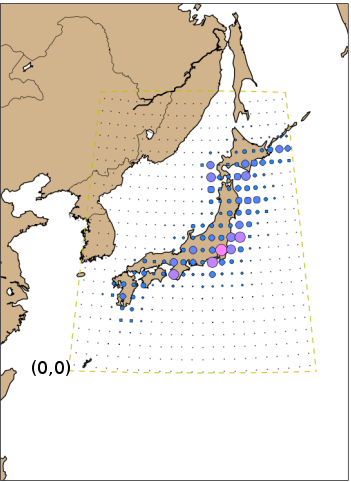
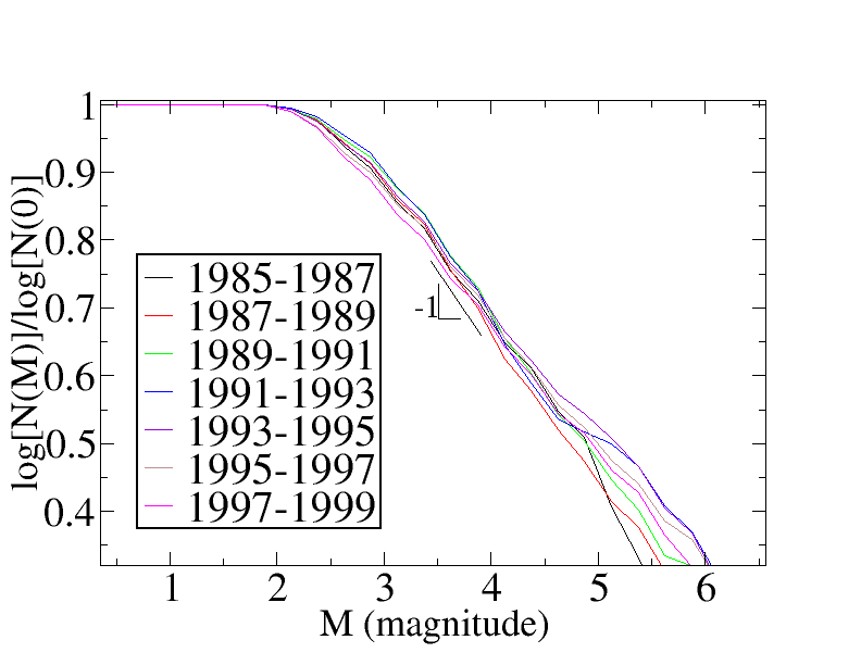
The data in the JUNEC catalog span 14 years from 1 July 1985 - 31 December 1998 and are depicted in Fig. 1. Each entry in the catalog includes the date, time, magnitude, latitude, and longitude of the event. We found the catalog to obey the Gutenberg-Richter law GRnote for events of magnitude 2.2 or larger. By convention, this is taken to mean that the catalog can be assumed to be complete in that magnitude range. However, because catalog completeness cannot be guaranteed for shorter time periods over a 14-year span, we also examine Gutenberg-Richter statistics for each non-overlapping two-year period (Fig. 2) GRnote . We find that, though absolute activity varies by year, the relative occurrences of quakes of varying magnitudes does not change significantly for events between magnitude 2.2 and 5, where there is the greatest danger of events missing from the catalog.
Additionally, the data are spatially heterogeneous, as shown in Fig. 1. Most events take place either over land or off Japan’s east coast. We remark to the reader that this is not an artifact of more detection equipment being located on land. The primary means for locating and detecting earthquake events involves using the S-waves and P-waves that emanate from the events. Seismic stations are capable of detecting these waves a great distance from their source. Both S-waves and P-waves waves travel through the Earth’s mantle, and the characteristic absorption distance, defined as the distance for wave amplitude to drop to of its original value, for body waves is on the order of 10,000 km lowrie . Any event of magnitude 5.5 or larger, for example, is detectable anywhere on earth. Hence, the location of the detection equipment does not affect how accurately events are catalogued. Additionally, because the location of the Japanese archipelago is a consequence of seismic activity involving the Philippine and other tectonic plates, it is not surprising that most seismic events take place on or near the islands themselves.
III Method
We partition the region associated with the JUNEC catalog as follows: we take the northernmost, southernmost, easternmost, and westernmost extrema of all events in the catalog as the spatial bounds for our analysis. We partition this region into a 23 23 grid which is evenly spaced in geographic coordinates. Each grid square of approximate size 100 km 100 km is regarded as a possible node in our network. Results do not qualitatively differ when the fineness of the spatial grid is modified, in agreement with analogous work carried out by Ref. lofti2012 , using a different technique from ours AS1 . However, 100 km boxes are a more physical choice, as 100 km is on the order of rupture length associated with earthquakes rupture , which in turn is roughly equivalent to the aftershock zone distance for larger earthquakes konst .
For a given measurement at time , an event of magnitude occurs inside a given grid square. Similar to the method of Corral corral , we define the signal of a given grid square to form a time series , where each series term is related to the earthquake activity that takes place inside that grid square within the time window , as described below.
Because events do not generally occur on a daily basis in a given grid square, it is necessary to bin the data to some level of coarseness. How coarse the data are treated involves a trade-off between precision and data richness.
We define the best results as those corresponding to the most prominent cross-correlations. To this end, we choose 90 days as the coarseness for our time series. This choice means that will cover a time window of days and will cover the 90-day non-intersecting time period immediately following, giving approximately 4 increments per year. Additional analysis shows that results do not qualitatively differ by changing the time coarseness.
We refer to the time series belonging to each grid cell as that grid cell’s signal. We define the signal that is related to the energy released in the the grid cell by
| (1) |
where denotes the number of events that occur in th time window in grid square . We choose this definition because the term is proportional to the energy released from an earthquake of magnitude M gupta . The signal therefore is proportional to the total energy released at a given location in a 90-day time period strain .
To define a link between two grid squares, we calculate the Pearson product-moment correlation coefficient between the two time series associated with those two grid squares feller
| (2) |
where indicates the mean and the standard deviations of the time series .
We consider the two grid squares linked if is larger than a specified threshold value , where is a tunable parameter. As is standard in network-related analysis, we define the degree of a node to be the number of links the node has. Note that our signal definition Eq. 1 involves an exponentiation of numbers of order 1. This means that the energy released, and therefore the cross-correlation between two signals, is dominated by large events. Examples of signals with high correlation are shown in Fig. 3.
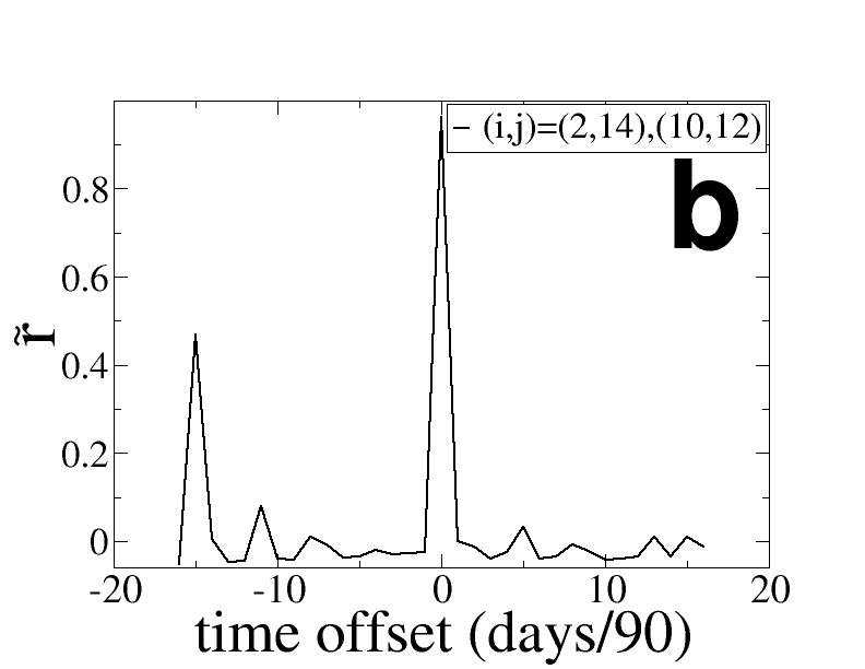
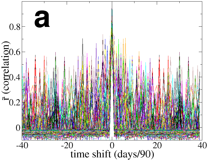
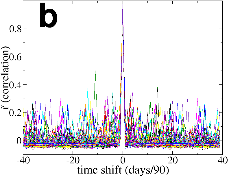
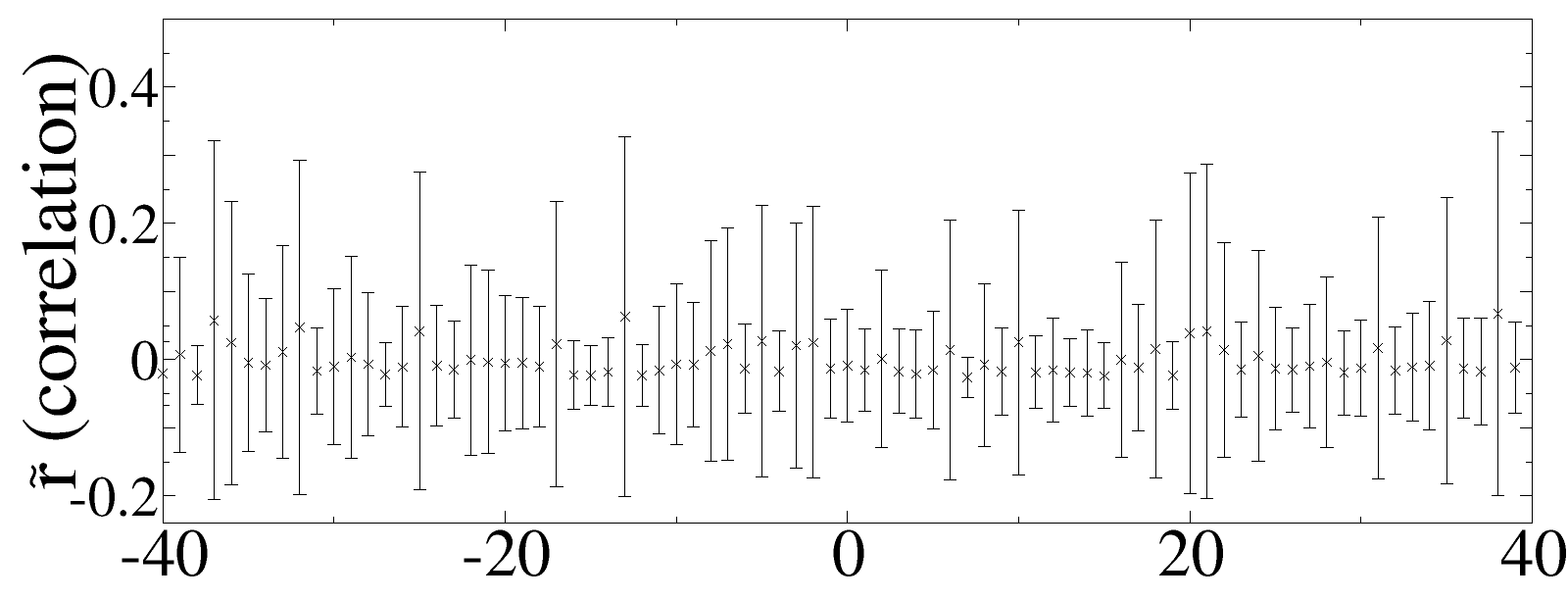
To confirm the statistical significance of , we compare of any two given signals with calculated by shuffling one of the signals. We also compare with the cross-correlation we obtain by time-shifting one of the signals by varying time increments ,
| (3) |
where is in units of 90 days. Further, we impose periodic boundaries
| (4) |
where is the length of the series. Our justification for these boundaries is that events in the distant past (10 years) should have nominal effects on the present, while they also provide typical background noise for comparison.
We note that over 14-year time period 1985-1998, the overall observed activity increases in the areas covered by the catalog. To ensure that the values we calculate are not simply the result of trends in the data, we compare our results to those obtained with linearly detrended data linear . We find that the trends do not have a significant effect. For example, using , we obtain 815 links, while detrending the data results in only 3 links dropping below the threshold correlation value. For , we obtain 1003 links, while detrending results in only 3 links dropped. Additionally, after detrending, 94% of correlation values stay within 2% of their values.
IV Results
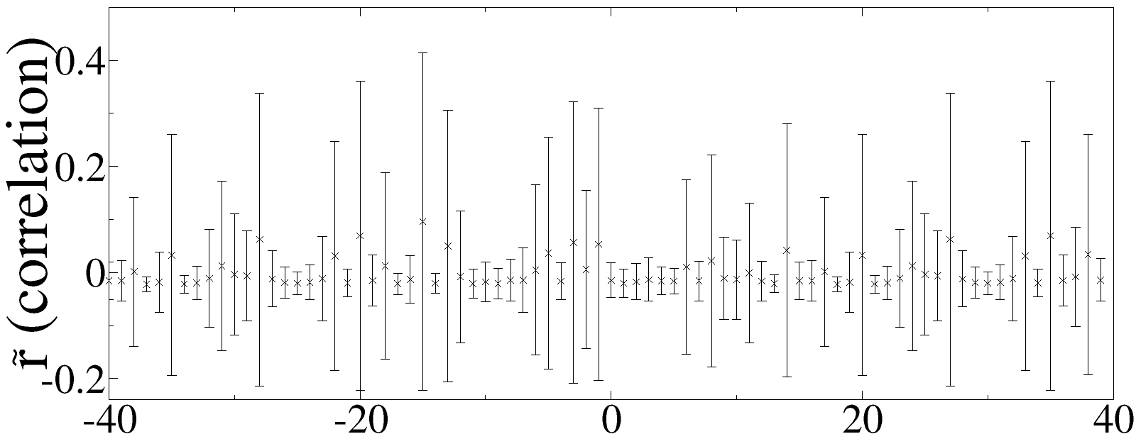
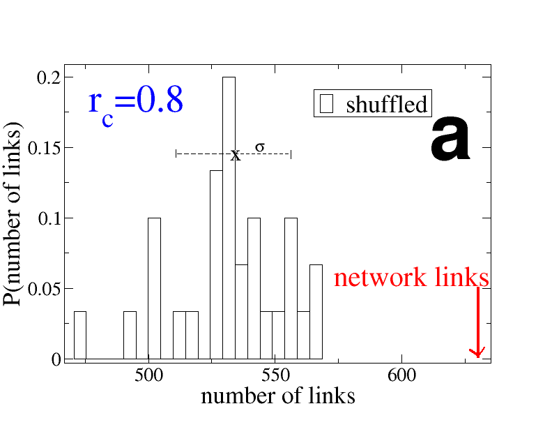
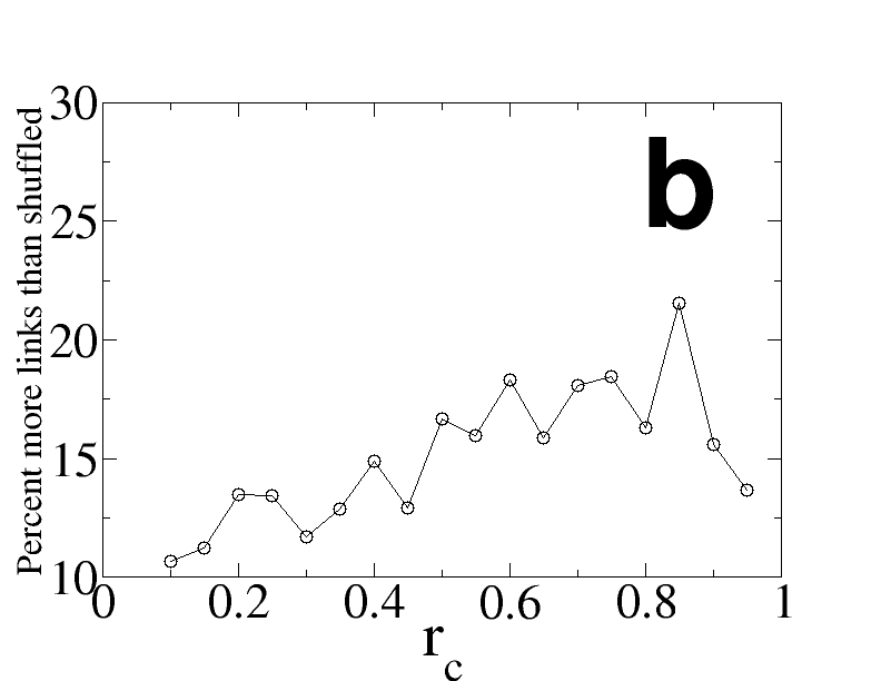
As described above, we compare of Eq. 3 between signals at different locations at the same point in time with and with with correlation coefficient obtained by shuffling one of the series. Shuffling or time-shifting by a single time step (representing 90 days) reduces to within the margin of significance, as shown in Fig. 4. Shuffling the signal also reduce s We find a large number of links with cross-correlations far larger than their shuffled counterparts. The number of links exceeds that of time-shuffled data by roughly 3-8, depending on choice of as shown in Fig. 5 (a). However, as shown, there are still many links that can be regarded as the result of noise. We therefore further examine the difference between the number of links found in time-shuffled data and the number found in the original data (Fig. 5 (b)). We find that the fraction of “real” links in general increases with .
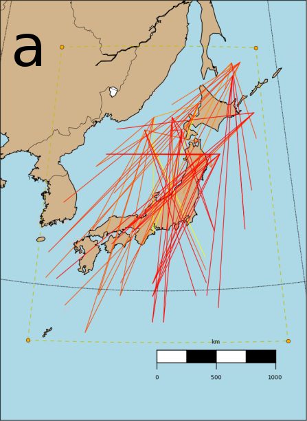
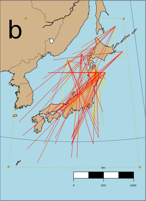
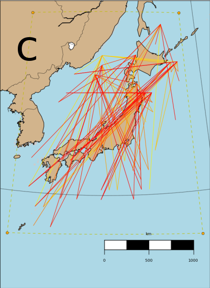
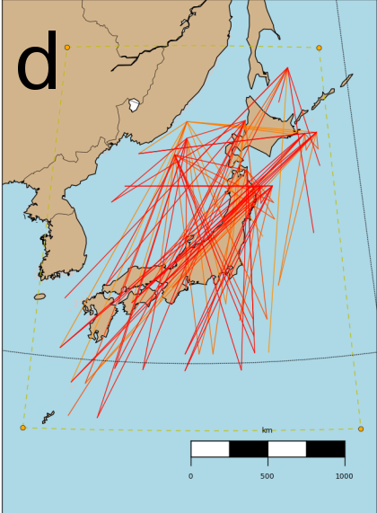
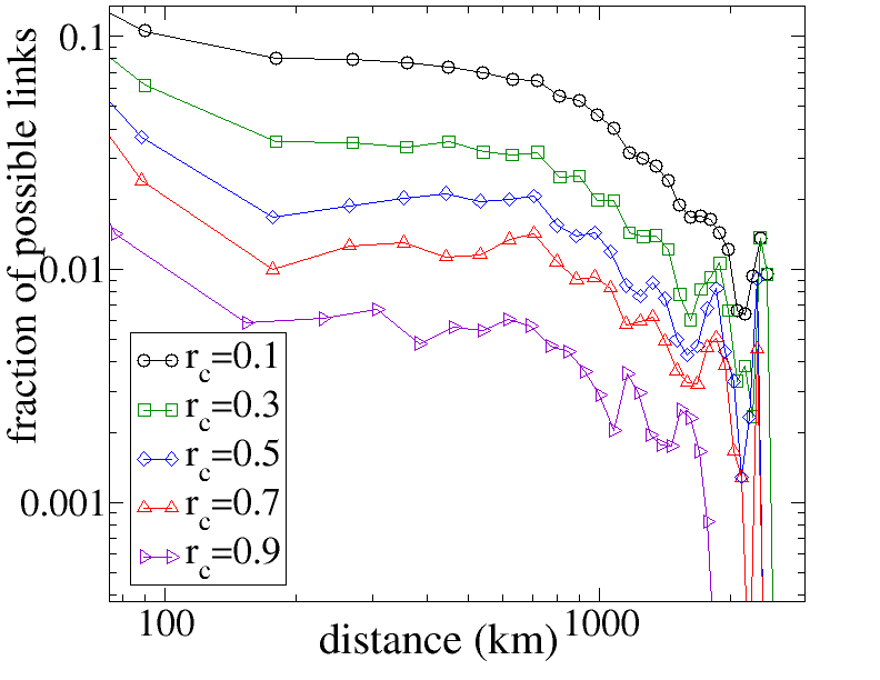
A significant fraction of these links connect nodes farther apart than 1000 km, as can be seen in Fig. 6. This is consistent with the finding that there is no characteristic cut-off length for interactions between events leastlikely ; lofti2012 , corroborated by Fig. 7, showing the number of links a network has at a given distance as a fraction of the number of links that are possible from choosing any two nodes in the potential network. Distances shorter than 100 km have sparse statistics due to the coarseness of the grid while distances greater than 2300 km have sparse statistics due to the finite spatial extent of the catalog. Within this range, the fraction of links observed drops off approximately no faster than a power law. We find qualitatively similar results when we adjust the grid coarseness.
Our results, shown in Fig. 6, are anisotropic, with the majority of links occurring at approximately 37.5 degrees east of north. This is roughly along the principal axis of Honshu, Japan’s main island, and parallel to the highly active fault zone formed by the subduction of the Philippine and Pacific tectonic plates under the Amurian and Okhotsk plates respectively. High degree nodes (i.e. nodes with a large number of links) tend to be found in the northeast and northcentral regions of the JUNEC catalog and are notably not strongly associated with the locations in the catalog that are most active, which we discuss in further detail below.
In network physics, we often characterize networks by the preference for high-degree nodes to connect to other high-degree nodes. The strength of this preference is quantified by the network’s assortativity, defined as
| (5) |
where is the Pearson correlation coefficient given by Eq. (2). The series and are found as follows: iterating through all entries in the adjacency matrix adj , the degree of each node is appended to the series and the degree of the node that is linked to is appended to the series . The assortativity coefficient thus gives a correlation of node degree within the network. If each node of degree connects only to nodes of the same degree, the two series and will be identical and A=1. Networks like the network of paper coauthorship have positive assortativity, while those of the World-Wide Web and of many ecological and biological systems have negative assortativity assortexamples .
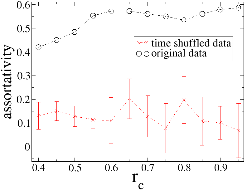
Fig. 8 shows that the networks resulting from our procedure are highly assortative with assortativity generally increasing with . The finding of positive correlation between the degree of a node and the degree of its neighbors is consistent with an analogous finding lofti2012 with Iranian data, using a different technique from ours AS1 . For comparison we show the assortativity obtained by using time shuffled networks. Since assortativity of the original networks is far higher than those of shuffled systems, the high assortativity cannot be due to a finite size effect or to the spatial clustering displayed in the data, since time shuffling preserves location. We investigate the nature of the high-degree nodes and find that high degree is not a matter of more events being nearby, as there is a slight tendency for higher degree nodes to actually have longer distance links on average than low degree nodes. Additionally, we found that node degree is essentially independent of both maximum earthquake size and number of events.
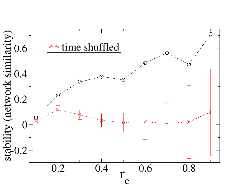
Because Fig. 5 shows, as mentioned above, that many links can be regarded as the result of noise, we investigate the stability of links over time (Fig. 9). Similarity of the network between the first seven years (1985-1992) and the second seven years (1992-1998) in the catalog is found as follows. We find the set of links that satisfy in both the 1985-1992 network and the 1992-1998 network, and create a series out of the respective link strengths (correlations) in the 1985-1992 network. We create another series using the same links, now using the corresponding strengths from the 1992-1998 network. We then correlate the two series using the Pearson correlation coefficient given by Eq. (2). We find that the network is far more stable over time than counterpart results given by shuffling the time series (Fig. 9). Because one would expect large correlations that arise purely from noise to have no “memory” from one time period to another, the finding of network stability over several years is consistent with our result that these links are not simply the result of chance.
V Discussion and conclusions
To summarize our results, we have introduced a novel method for analyzing earthquake activity through the use of networks signals . The resulting networks (i) display links with no characteristic length scale, (ii) display far more links than expected from chance alone, (iii) are far more assortative, and (iv) display significantly more link stability over time. The lack of a characteristic length scale is consistent with previous work and underscores the difficulty in making accurate predictions. The statistically significant nature of all of these results is consistent with the possibility of the presence of hidden information in a catalog, not captured by existing models or previous earthquake network approaches.
We thank K. Yamasaki for useful discussions, and the DTRA, ONR, European EPIWORK and LINC projects, and the Israel Science Foundation for financial support.
References
- (1) Y. Y. Kagan and D. D. Jackson, J. Geophys. Res. 96, 419 (1991).
- (2) D. Marsan, C. J. Bean, S. Steacy, and J. McCloskey, J. Geophys. Res. 105, 28081 (2000).
- (3) B. Gutenberg and C.F. Richter, Bull. Seismol. Soc. Am. 34, 185 (1944).
- (4) F. Omori, J. Coll. Sci. Imp. Univ. Tokyo 7, 111 (1894); see the recent work of M. Bottiglieri, L. de Arcangelis, C. Godano, and E. Lippiello, Phys. Rev. Lett. 104, 158501 (2010).
- (5) T. Utsu, Geophys. Magazine 30, 521 (1961).
- (6) T. Utsu, Y. Ogata, R. S. Matsu’ura. J. of Phys. of the Earth 43, 1 (1995).
- (7) M. Bath, Tectonophysics, 2, 483 (1965).
- (8) Y. Y. Kagan and L. Knopoff, Geophys. J. R. Astron. Soc. 62, 303 (1980).
- (9) D. Turcotte, Fractals and Chaos in Geology and Geophysics (Cambridge University Press, Cambridge, 1997).
- (10) P. G. Okubo and K. J. Aki, J. Geophys. Res. 92, 345 (1987).
- (11) T. Hirata, Pure and Applied Geophysics, 131, 157 (1989).
- (12) P. Bak, K. Christensen, L. Danon, and T. Scanlon, Phys. Rev. Lett. 88, 178501 (2002).
- (13) A. Corral, Phys. Rev. E 68, 035102(R) (2003).
- (14) R. Olsson, Geodynamics 27, 547 (1999).
- (15) S. Abe and N. Suzuki, J. Geophys. Res. 108, 2113 (2003).
- (16) S. Abe and N. Suzuki, Physica A 332, 533 (2004).
- (17) S. Abe and N. Suzuki, Physica A 350, 588 (2005).
- (18) S. Abe and N. Suzuki, Eur. Phys. J. B 59, 93–97 (2007).
- (19) J. Davidsen, P. Grassberger, and M. Paczuski, Geophys. Res. Lett. 33, L11304 (2006); Phys. Rev. E 77, 066104 (2008).
- (20) N. Lotfi and A. H. Darooneha, Eur. Phys. J. B 85, 23 (2012).
- (21) D. Pastén, S. Abe, V. Muñoz, and N. Suzuki, arXiv:1005.5548v1 (2010).
- (22) S. Abe, D. Pastén, and N. Suzuki, Physica A 390, 1343 (2011).
- (23) M. Baiesi and M. Paczuski, Phys. Rev. E 69, 066106 (2004).
- (24) V. N. Livina, S. Havlin, and A. Bunde, Phys. Rev. Lett. 95, 208501 (2005).
- (25) E. Lippiello, L. de Arcangelis, and C. Godano, Phys. Rev. Lett. 100, 038501 (2008).
- (26) S. Lennartz, V. N. Livina, A. Bunde, and S. Havlin, Europhys. Lett. 81, 69001 (2008).
- (27) A. Corral, Phys. Rev. Lett. 92, 108501 (2004).
- (28) D. Sornette and L. Knopoff, Bull. Seismol. Soc. Am. 87, 789 (1997).
- (29) J. Davidsen and C. Goltz, Geophys. Res. Lett. 31, L21612 (2004).
- (30) The Gutenberg-Richter law states that the number of events in the catalog greater that a certain magnitude has an exponential dependence, i.e. , where and are empirically observed constants with typically .
- (31) P-waves and S-waves are the body waves which originate at an earthquake and travel through the earth. They are the primary means for locating an event. See: K. E. Bullen and B. A. Bolt, An Introduction to the Theory of Seismology (Cambridge University Press, Cambridge, 1993).
- (32) W. Lowrie, Fundamentals of Geophysics p.98 (Cambridge University Press, Cambridge, 2007).
- (33) D. L. Wells and K. H. Coppersmith, Bull. Seismol. Soc. Am. 84, 974 (1994).
- (34) K. I. Konstantinoua, G. A. Papadopoulos, A. Fokaefs, K. Orphanogiannaki, Tectonophysics 403, 95 (2005).
- (35) K. Arora, A. Cazenave, E. R. Engdahl, R. Kind, A. Manglik, S. Roy, K. Sain, S. Uyeda, and H. K. Gupta, Encyclopedia of Solid Earth Geophysics, Volume 1, p.213 (Springer, 2011).
- (36) We note that this term is similar in appearance though distinct from the cumulative Benioff strain bowman , the predictive power of which is hotly contested in geophysics felzer ; hardebeck . However, our technique does not use this term to make predictive statements about any individual events in a specific location, but rather allows us to observe patterns in the similarity of behavior across different locations.
- (37) To detrend the data, we obtain a best fit linear trend for each time series and subtract it from the series. We calculate the cross-correlation between the detrended sequences.
- (38) The adjacency matrix fully specifies a given network. denotes a link between node and node while denotes no link.
- (39) M. E. J. Newman, Phys. Rev. Lett. 89, 208701 (2002).
- (40) W. Feller, An Introduction to Probability Theory and Its Applications, San Diego, 1997, edited by J. B. Kadtke, A. Bulsara (AIP, Woodbury, 1997).
- (41) For comparison, we also carried out our analysis with another three signal definitions that we omit here: (1) “average magnitude”: , where is the magnitude of the event and is the total number of events occurring in the 90-day time window in the grid square . (2) “number of events”: , with the symbols as defined in (a). (3) “magnitude sum”: . All three of these alternative definitions fail to give results significantly better than the shuffled data that are robust with respect to the various adjustable parameters.
- (42) D. D. Bowman, G. Ouillon, C. G. Sammis, A. Sornette, and D. Sornette, J. Geo-phys. Res. 103, 24,359 (1998).
- (43) K. R. Felzer, T. W. Becker, R. E. Abercrombie, G Ekstrom, J. R. Rice, J. Geophys. Res. 107, 2190 (2002).
- (44) J. L. Hardebeck, K. Felzer, and A. J. Michael, J. Geophys. Res. 113, B08310 (2008).