Abstract

A graph based matching is used to construct aggregation based coarsening for algebraic multigrid method. Effects of inexact coarse grid solve is analyzed numerically for a highly discontinuous convection-diffusion coefficient matrix, and for problems from Florida matrix market collection. The proposed strategy is found to be more robust compared to a classical AMG approach.

1 Introduction

We concern ourselves with the problem of solving large sparse linear system of the form

$$Ax=b,$$ (1)

arising from the cell centered finite volume discretization of the convection diffusion equation as follows

$$\text{div}(\mathbf{a}(x)u)-\text{div}(\kappa(x)\nabla u) = f~{}\text{in}~{}\Omega,$$

$$u = 0~{}\text{on}~{}\partial\Omega_{D},$$ (2)

$$\frac{\partial u}{\partial n} = 0~{}\text{on}~{}\partial\Omega_{N},$$

where $\Omega=[0,1]^{n}$ ($n=2$, or 3), $\partial\Omega_{N}=\partial\Omega\setminus\partial\Omega_{D}.$ The vector field $\mathbf{a}$ and the tensor $\kappa$ are the given coefficients of the partial differential operator. In 2D case, we have $\partial\Omega_{D}=[0,1]\times\{0,1\}$, and in 3D case, we have $\partial\Omega_{D}=[0,1]\times\{0,1\}\times[0,1]$. Other sources include problems from Florida matrix market collection [9]; see Table (3) for a list of problems considered in this paper.

Currently, one of the most successful methods for these problems are the multigrid methods (MG) [21, 25, 26]. The robustness of the multigrid method is significantly improved when they are used as a preconditioner in the Krylov subspace method [22]. If $B$ denotes the MG preconditioner then the preconditioned linear system is the transformation of the linear system (1) to $B^{-1}Ax=B^{-1}b$. Here $B$ is a preconditioner which an approximation to the matrix $A$ such that the spectrum of $B^{-1}A$ is “favourable” for the faster convergence of Krylov methods. For instance, if the eigenvalues are clustered and are sufficiently close to one, then a fast convergence is observed in practice. Furthermore, the preconditioner B should be cheap to build and apply. With the advent of modern day multiprocessor and multicore era, the proposed method should have sufficient parallelism as well.

In multigrid like methods, the problem is solved using a hierarchy of discretizations; the finest grid is at the top of the hierarchy followed by coarser grids. The two complementary processes are: smoothening and coarse grid correction. The smoothers are usually chosen to be the classical relaxation methods such as Jacobi, Gauss-Seidel, or incomplete LU methods [22]. Analysis for model problems reveals that the smoothers efficiently eliminates the low frequency part of the error, while the global correction which is obtained by solving a restricted problem on the coarser grid damps the high frequency part of the error [30]. In fact, low frequency errors on the fine grid becomes high frequency error on the coarse grid leading to their efficient resolution on the coarser grid. It is therefore crucial to choose efficient smoothers and a coarse grid solver. The classical geometric multigrid methods require informations on the grid geometry and constructs a restriction operator and a coarse grid. Since, a geometric multigrid method is closely related to the grid, the problem with nonlinearity can be resolved efficiently. But, for a complex grid, the applicability of the method becomes increasingly difficult. On contrary, algebraic multigrid method defines the necessary ingredients based solely on the coefficient matrix. Much research have been devoted to algebraic multigrid methods and several variants exists.

In this paper, an aggregation based algebraic multigrid is proposed. The aggregation is based on graph matching. This is achieved by partitioning the graph of the matrix such that the partitioned subgraphs are assumed to be the aggregates. Once a set of aggregates is defined, the coarse grid is constructed from the Galerkin formula. In [11], authors use graph partitioner to form aggregates, and forward Gauss-Seidel with downwind numbering is used as pre- and post-smoother with the usual recursive multigrid method, where the coarsening is continued untill the number of unknowns in the coarse grid are less than 10. This approach may lead to a deep hierarchy of grids, thus making the method very recursive and less adapted to modern day multi-processor or multi-core environment. In [20], similar graph based matching is used to form a coarse grid, and the classical recursive smoothed AMG approach is followed, however, here, ILUT [22] is used for pre- and post-smoothing.

Our aim in this work is to propose a strategy that tries to avoid deep recursion but combines several different approaches as above. The strategy we adopt has the following ingredients:

• Coarsening based on graph matching

• ILU(0) is the smoother with natural or nested dissection reordering

• Coarse grid equation is solved inexactly using ILUT

We show that the strategy proposed above is simple, easy to implement, and works well in practice for symmetric positive definite systems with large jumps in the coefficients. Solving a coarse grid inexactly leads to a faster and cheaper method. Indeed, a parallel incomplete coarse grid solve will be desirable, however, in this work, we consider only the sequential version. We provide an estimate of heurestic coarse grid size and an estimate of a parameter involved in the inexact coarse grid solve. We compare our approach with a classical AMG [19] with Gauss-Seidel smoothing and exact coarse grid solve.

The rest of the paper is organized as follows. In section (2), we discuss the classical coarsening strategy based on strength of connection, and the one based on graph matching. The numerical experiments are presented in section (3); the proposed method is compared with a classical AMG method on discontinous convection-diffusion problems and some problems from Florida matrix market collection [9]. Finally, section (4) concludes the paper.

2 Graph matching based aggregation for AMG

In a typical two grid method, there are two complementary processes namely, a smoother and a coarse grid correction step. When this strategy is repeated by creating another coarser grid, then the method is known as multigrid. During a fixed point iterative process, the high frequency components of the error or the so called rough part are dealt with efficiently by a smoother. On the other hand, the low frequency components of the error can only with dealt with globally by a method that is “connected” globally (pertains to global fine grid). We imagine the coefficients of the matrix as an approximation to some function (Jacobian in case of nonlinear iteration). For an example, assuming that a linear function is sufficiently smooth, an approximation to the function with $N$ discrete points is close to an approximation to the function with only $N/2$ (or even $N/4$) discrete points. Thus, we solve the problem cheaply with $N/2$ grid points (i.e, on a coarser grid) and then we interpolate the solution to obtain an approximation to the problem defined on $N$ grid points. The error in the solution thus obtained has rough components because they were not taken into account properly while solving with the coarse solver, and this is where smoother comes into play. This interplay of smoother and coarse grid correction are complementary. For a more rigorous explanation, an inclined reader is referred to [21, 25, 26] where tools from Fourier analysis is used to explain why smoothening and coarse grid correction step works effectively for some problems.

In classical AMG, a set of coarse grid unknowns is selected and the matrix entries are used to build interpolation rules that define the prolongation matrix P, and the coarse grid matrix $A_{c}$ is computed from the following Galerkin formula

$$A_{c}=P^{T}AP.$$ (3)

In contrast to the classical AMG approach, in aggregation based multigrid, first a set of aggregates $G_{i}$ are defined. Let $N_{c}$ be the number of such aggregates, then the interpolation matrix $P$ is defined as follows

$$P_{ij}=\begin{cases}1,&\text{if $i\in G_{j}$,}\\ 0,&\text{otherwise,}\\ \end{cases}$$

Here, $1\leq i\leq N,\,1\leq j\leq N_{c}$, $N$ being the size of the original coefficient matrix $A$. Further, we assume that the aggregates $G_{i}$ are such that

$$G_{i}\cap G_{j}=\phi,~{}\text{for}~{}i\neq j~{}\text{and}~{}\cup_{i}G_{i}=[1,N]$$ (4)

Here $[1,\,N]$ denotes the set of integers from $1$ to $N$. Notice that the matrix $P$ defined above is an $N\times N_{c}$ matrix, but since it has only one non-zero entry (which are “one”) per row, the matrix can be defined by a single array containing the indices of the non-zero entries. The coarse grid matrix $A_{c}$ may be computed as follows

$$(A_{c})_{ij}=\sum_{k\in G_{i}}\sum_{l\in G_{j}}a_{kl}$$

where $1\leq i,\ j\leq N_{c}$, and $a_{kl}$ is the $(k,l)th$ entry of $A$.

Numerous aggregation schemes have been proposed in the literature, but in this paper we consider two of the aggregation schemes as follows

Aggregation based on strength of connection: This approach is closely related to the classical AMG [26] where one first defines the set of nodes $S_{i}$ to which $i$ is strongly negatively coupled, using the Strong/Weak coupling threshold $\beta$:

$$S_{i}=\{\,j\neq i\mid a_{ij}<-\beta\ \text{max}|a_{ik}|\,\}.$$

Then an unmarked node $i$ is chosen such that priority is given to the node with minimal $M_{i}$, here $M_{i}$ being the number of unmarked nodes that are strongly negatively coupled to $i$. For a complete algorithm of the coarsening, the reader is referred to [19].

Aggregation based on graph matching: Several graph partitioning methods exists, notably, in software form [12, 14, 23]. Aggregation for AMG is created by calling a graph partitioner with required number of aggregates as an input. The subgraph being partitioned are considered as aggregates. For instance, in this paper we use this approach by giving a call to the METIS graph partitioner routine METIS_PartGraphKway with the graph of the matrix and number of partitions as input parameters. The partitioning information is obtained in the output argument “part”. The part array maps a given node to its partition, i.e., part($i$) = $j$ means that the node $i$ is mapped to the $jth$ partition. In fact, the part array essentially determines the interpolation operator $P$. For instance, we observe that the ”part“ array is a discrete many to one map. Thus, the $i$th aggregate $G_{i}=\text{part}^{-1}(i)$, where

$$\text{part}^{-1}(i)=\{\,j\in[1,\,N]\enspace\mid\enspace\text{part}(j)=i\,\}$$

Such graph matching techniques were explored in [6, 11, 20]. For notational convenience, the method introduced in this paper will be called GMG (Graph matching based aggregation MultiGrid).

Let $S$ denote the matrix which acts as a smoother in GMG method. The usual choice of $S$ is a Gauss-Siedel preconditioner [22]. However, in this paper we choose ILU(0) as a smoother, we find that the choice of ILU(0) as a smoother gives more robustness compared to Gauss-Siedel method, however, at an additional storage cost. Another aspect that we explore is to use only two grid approach but with an incomplete coarse grid solve. That is, we use an incomplete ILU($t$), where $t$ is the tolerance for dropping the entries, see [22]. The approximation $\tilde{A}_{c}$ of the coarse grid operator $A_{c}$ is given as follows

$$\tilde{A}_{c}=\tilde{L}_{c}\tilde{U}_{c},~{}\text{where},~{}[\tilde{L}_{c},\tilde{U}_{c}]=\text{ILUT}(A_{c})$$

where ILUT stands for ILU($t$). The reason for using only two grid, and using an incomplete (and possibly parallel) coarse grid solve is to avoid the recursion in the the typical AMG method. It may be profitable to solve the coarse grid problem in parallel and inexactly, when the problem size becomes large. This may be achieved by a call to one of the several hybrid incomplete solvers based on ILU [2] like approximation or by using a sparse approximate inverse [5]. The investigation with the parallel inexact approximation of the coarse solver will be done in future, and in this paper, we shall understand the qualitative behavior such as the convergence and robustness of the proposed strategy compared to a classical AMG approach found in [16].

Let $M=PA_{c}P^{T}$ denote the coarse grid operator interpolated to fine grid, then the two-grid preconditioner without post-smoothing is defined as follows

$$B=(S^{-1}+M^{-1}-M^{-1}AS^{-1})^{-1}.$$ (5)

We notice that $M^{-1}\approx PA_{c}^{-1}P^{T}$, thus, an equation of the form $Mx=y$ is solved by first restricting $y$ to $y_{c}=P^{T}y$, then solving with the coarse matrix $A_{c}$ the following linear system: $A_{c}x_{c}=y_{c}$. Finally, prolongating the coarse grid solution $x_{c}$ to $x=Px_{c}$. Following diagram illustrates the two-grid hierarchy.

The preconditioner $B$ is similar to the combination preconditioner defined in [1, 13], where instead of defining a coarse grid operator a deflation preconditioner is used. Thus, rather than satisfying a “filtering property”, the coarse grid operator satisfies the following “approximate filtering condition (AFC)”

$$AP\approx MP,\quad\text{(see Theorem (\ref{filter}) on page \ref{filter})},$$

where columns of interpolation matrix $P$ spans a subspace of dimension $N_{c}$. Here, we have considered the exact coarse grid solve, the inexact version is similar to the exact two-grid preconditioner (5) defined above except that $M$ is replaced by $\tilde{M}=P\tilde{A}_{c}P^{T}$, and we denote the inexact two grid preconditioner by $\tilde{B}$. In Algorithm (1), we present the complete iterative algorithm for the inexact case; the algorithm is essentially a slightly modified form of algorithm presented in Figure (2.6) in [4]. The two-grid methods can also be integrated in a similar way in an iterative accelerator other than GMRES, to integrate with other accelerators, see [4].

Algorithm 1 PSEUDOCODE TO SOLVE $Ax=b$, $A\in\mathbb{R}^{N\times N}$, $x,\,b\in\mathbb{R}^{N}$

   OBJECTIVE: To solve Ax = b

  SETUP PHASE

  Call graph partitioner to get partitions in an array, say, part.

  Use part array to form aggregates $G_{i}$ and the prolongation matrix $P$ (subgraphs are aggregates)

  Create coarse grid matrix $A_{c}\in\mathbb{R}^{N_{c}\times N_{c}}$ as follows

$$(A_{c})_{ij}=\sum_{k\in G_{i}}\sum_{l\in G_{j}}a_{kl}.$$

  Factor the coarse grid matrix inexactly: $\tilde{A}_{c}=\text{ILUT}(A_{c})$. Here ILUT is incomplete LU with tolerance.

  Setup smoother: $S=L_{0}U_{0}=\text{ILU0}(A)$. Here ILU0 is incomplete LU with zero fill-in

  Define (not to be formed explicitely) two-grid preconditioner $\tilde{B}$ and $\tilde{M}$ as follows

$$\tilde{B}=(S^{-1}+\tilde{M}^{-1}-\tilde{M}^{-1}AS^{-1})^{-1},\quad\tilde{M}=P\tilde{A_{c}}P^{T}$$

  PRECONDITIONED GMRES ITERATION

  $x_{0}$ is an initial guess

  for $j=1,2,\dots$ do

     Solve $r$ from $\tilde{B}r=b-Ax_{0}$ (See SOLVE $\tilde{B}q=z$ function below)

     $v^{(1)}=r/\|r\|_{2},\quad s:=\|r\|_{2}e_{1}$

     for $i=1,2,\dots,m$ do

        Solve $w$ from $\tilde{B}w=Av^{(i)}$ (See SOLVE $\tilde{B}q=z$ function below)

        for $k=1,\dots,i$ do

           $h_{k,i}=(w,v^{(k)}),\quad w=w-h_{k,i}v^{(k)}$

        end for

        $h_{i+1,i}=\|w\|_{2},\quad v^{(i+1)}=w/h_{i+1,i}$

        apply $J_{1},\dots,J_{i-1}$ on ($h_{1,i},\dots,h_{i+1,i}$)

        construct $J_{i}$, acting on the $i$th and $(i+1)$st component of $h_{.,i}$, such that $(i+1)$st component of $J_{i}h_{.,i}$ is $0$

        set $s:=J_{i}s$

        if $s(i+1)$ is small enough then

           UPDATE($\tilde{x},i$) and quit

        end if

     end for

     UPDATE($\tilde{x},m$)

  end for

  UPDATE($\tilde{x},m$)

  Solve for $y$ in $Hy=\tilde{s}$. Here upper $i\times i$ part of $H$ has $h_{i,j}$ as its element. $\tilde{s}$ represents the first $i$ components of $s$

$$\tilde{x}=x^{(0)}+y_{1}v^{(1)}+y_{2}v^{(2)}+\dots+y_{i}v^{(i)},\quad s^{(i+1)}=\|b-A\tilde{x}\|_{2}$$

  If $\tilde{x}$ is accurate enough then quit else $x^{(0)}=\tilde{x}$

  SOLVE $\tilde{B}q=z$

  Solve $St=z$ (use $S=L_{0}U_{0}$), solve $\tilde{M}f=z$ (See SOLVE $\tilde{M}g=h$ function below), solve $\tilde{M}q=At$, set $q=t+f-q$

  SOLVE $\tilde{M}g=h$

  set $h_{c}=P^{T}h$, Solve $\tilde{A}_{c}g_{c}=h_{c}$ (use $\tilde{A}_{c}=\tilde{L}\tilde{U}$), $g=Pg_{c}$

2.1 Analysis of graph based two-grid method

For any matrix $K$, let $K\succ 0$ denote that the matrix $K$ is symmetric positive definite and we use the notation $K(:,j)$ to denote the $j$th column of $K$, whereas, $K(j,:)$ to denote the $j$th row of $K$. If $A\succ 0$, then the inner product $(\,,\,)_{A}$ defined by $(u,v)_{A}=u^{T}Av$ is a well defined inner product, and it induces the energy norm $\|\,\|_{A}$ defined by $\|v\|_{A}=(v,v)_{A}^{1/2}$ for any vector $v$. A matrix $K$ is called A-selfadjoint if

$$(Ku,v)=(u,Kv)_{A},$$

or equivalently if

$$A^{-1}K^{T}A=K.$$

For any matrix $K$, let span($K$) denote a set of all possible linear combination of the columns of the matrix $K$. Let $\|x\|$ denote the Euclidean norm ($\sum_{i=1}^{n}x_{i}^{2})^{\frac{1}{2}}$. In what follows, we assume that the matrix $P$ is orthonormalized, such that $P^{T}P=I$. The basic linear fixed point method for solving the linear systems (1) is given as follows

$$x^{n+1}=x^{n}+B^{-1}(f-Ax^{n})=(I-B^{-1}A)u^{n}+B^{-1}b$$

Subtracting the equation above with the identity $x=x-B^{-1}Ax+B^{-1}b$ yields the following equation for the error $e^{n+1}=u-u^{n}$

$$e^{n+1}=(I-B^{-1}A)e^{n}=(I-B^{-1}A)^{2}e^{n-1}=\dots=(I-B^{-1}A)^{n+1}e^{0}.$$

Choosing $B$ as in Equation (5), we have the following relation

$$e^{n+1}=(I-S^{-1}A)^{n+1}(I-M^{-1}A)^{n+1}e^{0}$$

Thus, the quality of the preconditioner $B$ depends on how well the smoother $S$ and the coarse grid preconditioner $M$ acts on the error.

In [1, 13, 27, 28, 29], a composite preconditioner similar to the one in (5) is proposed, where, the matrix $M$ is replaced by a preconditioner, say, $M_{f}$ that deflates the eigenvector corresponding to smaller eigenvalue. The preconditioner $M_{f}$ is constructed such that it satisfies a “filtering property” as follows

$$M_{f}t=At,$$

where $t$ is a filter vector. In [1], the filter vector is choosen to be a Ritz vector corresponding to smallest Ritz value in magnitude obtained after a couple of iterations of ILU(0) preconditioned matrix. In [27], first the iteration is started with a fixed set of filter vector, and later the filter vector is changed adaptively using error vector. In [13], authors fixed the filter vector to be a vector of all ones and show that the composite preconditioner is efficient for a range of convection-diffusion type problems. In brief, for an effective method, the columns of the interpolation matrix $P$ should approximate well the eigenvectors corresponding to low eigenvalues. One possibility is to use $P$ to construct a deflation preconditioner as shown in [17].

The following theorem shows that preconditioner $M$ that corresponds to a coarse grid correction step satisfies a more general but approximate filtering condition.

Theorem 1.

If the coarse grid correction preconditioner $M=PA_{c}P^{T}$ and the coarse grid operator $A_{c}=P^{T}AP$ are nonsingular, then following holds:

1. $MP\approx AP$

2. If $t=[1,1,\dots,1]$, then $t\in span(P)$ and dim(span(P)) = $N_{c}$

Proof.

We have

$$(I-M^{-1}A)P \approx P-P{A_{c}}^{-1}P^{T}AP$$

$$=P-P{A_{c}}^{-1}A_{c}$$

$$=0$$

From equations (2) and (4), we find that $P$ is an $N\times N_{c}$ matrix, and the $j$th column of the matrix $P$ has a non-zero entry $P(i,j)=1$ if and only if $i\in G_{j}$. Since the aggregates $G_{j}^{\prime}s$ cover all the nodes in the set $[1,N]$, for all $i\in[1,N]$, there exists an aggregate $G_{j}$ such that $i=G_{j}(k)$ for some $k$, and consequently $P(i,j)=1$. Moreover, since the aggregates $G_{j}^{\prime}s$ do not intersect, such $j$ is unique. In other words, for each $i\in[1,N]$, there exists one and only one column $P(:,j)$ of $P$ such that the $i$th entry of column $P(:,j)$ is 1. Hence we have

$$Pt=\sum_{1\leq i\leq N_{c}}P(:,j)=t$$

and since each columns of $P$ are linearly independent we have dim(span(P)) = $N_{c}$. ∎

Theorem 2.

If $A\succ 0$, then $A_{c}\succ 0$.

Proof.

We have $A_{c}=P^{T}AP$ and

$$(A_{c}x,x) = (P^{T}APx,x),~{}\text{for}~{}x\neq 0$$

$$= (APx,Px),~{}\text{for}~{}x\neq 0$$

$$> 0,~{}\text{for}~{}x\neq 0.$$

Notice that we use the fact that $P$ is a boolean matrix, i.e., it has one and only one non-zero entry equal to “one” per row. Thus, $Px\neq 0$ for $x\neq 0,~{}x\in R^{N_{c}}$. Hence the theorem. ∎

However, the global preconditioner corresponding to the coarse grid solve represented by $M=PA_{c}P^{T}$ or $M^{-1}A$ is not necessarily SPD. We have the following counter examples

Theorem 3.

$A\succ 0$ does not imply that $M\succ 0$ or $M^{-1}A\succ 0$.

Proof.

Let $N=4$ be the size of $A$. Let there be two aggregates, $G_{1}=\{\,1,3\,\}$ and $G_{2}=\{\,2,4\,\}$, then the restriction operator $P^{T}$ is defined as follows $P^{T}=\left[\begin{array}[]{cccc}1&0&1&0\\ 0&1&0&1\end{array}\right]$, choosing $x^{T}=[1,0,-1,0]$, we have $P^{T}x=0$. Thus, we have

$$(Mx,x)\not>0,\quad(M^{-1}Ax,x)\not>0~{}\text{for all $x\neq 0$}.\qed$$

In literature, much results have been proved when the coefficient matrix is a diagonally dominant $M-$matrix. We collect some relevant results, and use them to understand the proposed method.

Definition 1.

Let $G(A)=(V,E)$ be the adjacency graph of a matrix $A\in\mathbb{R}^{N\times N}$. The matrix $A$ is called irreducible if any vertex $i\in V$ is connected to any vertex $j\in V$. Otherwise, $A$ is called reducible.

Definition 2.

A matrix $A\in\mathbb{R}^{N\times N}$ is called an $M-$matrix if it satisfies the following three properties:

1. $a_{ii}>0$ for $i=1,\dots,N$

2. $a_{ij}\leq 0$ for $i\neq j$, $i,j=1,\dots,N$

3. $A$ is non-singular and $A^{-1}\geq 0$

Definition 3.

A square matrix $A$ is strictly diagonally dominant if the following holds

$$|a_{ii}|>\sum_{j\neq i}|a_{ij}|,i=1,\dots,N$$

and it is called irreducibly diagonally dominant if $A$ is irreducible and the following holds

$$|a_{ii}|\geq\sum_{j\neq i}|a_{ij}|,i=1,\dots,N$$

where strict inequality holds for atleast one $i$.

A simpler criteria for $M-$matrix property is given by the following theorem.

Theorem 4.

If the coefficient matrix $A$ is strictly or irreducibly diagonally dominant and satisfies the following conditions

1. $a_{ii}>0$ for $i=1,\dots,N$

2. $a_{ij}\leq 0$ for $i\neq j$, $i,j=1,\dots,N$

then $A$ is an $M-$matrix.

Theorem 5 ([11]).

If $A\in\mathbb{R}^{N\times N}$ is a strictly or irreducibly diagonally dominant $M-$matrix, then so is the coarse grid matrix $A_{c}=P^{T}AP$.

Proof.

The theorem is proved in [11]. ∎

Theorem 6 ([15]).

If the coefficient matrix $A$ is symmetric $M-$matrix, and let $S=\tilde{L}\tilde{L}^{T}$ be the incomplete cholesky factorization, then the fixed point iteration with the error propogation matrix $I-S^{-1}A$ is convergent.

Theorem 6 above tells us that for an M-matrix, ILU(0) preconditioned method will be convergent by itself. However, the convergence is usually slow due to large iteration count with increasing problem size. Combining ILU(0) with a coarse grid correction leads to convergence rate which depends mildly on the problem size. Following result shows that the inexact factorization is as stable as the exact factorization of the coarse grid operator.

Theorem 7.

If the given coefficient matrix $A$ is a symmetric irreducibly diagonally dominant $M-$matrix, and if the inexact coarse grid operator $\tilde{A}_{c}$ is based on incomplete LU factorization as follows

$$\tilde{A}_{c}=\textup{CHOLINC}(A_{c}),$$

where CHOLINC is the incomplete Cholesky factorization, then the construction of $\tilde{A}_{c}$ is atleast as stable as the construction of an exact decomposition of $A_{c}$ without pivoting.

Proof.

If the original matrix $A$ is symmetric and irreducibly diagonally dominant $M-$matrix, then Theorem 5 tells us that the coarse grid operator $A_{c}$ obeys the same property. Now, $A_{c}$ being an $M-$matrix, Theorem 3.2 in [15] tells us that $\tilde{A}_{c}$ defined above is as stable as the exact Cholesky factorization of $A_{c}$. ∎

For a diagonally dominant $M$-matrix, pivoting is rarely needed. However, pivoting generally improves the stability of incomplete LU type factoriations. This is the reason why we use incomplete LU with pivoting, namely, ILUT function of MATLAB. Moreover, using ILUT will lead to a method suitable for unsymmetric matrices that are not necessarily diagonally dominant. We refer the curious reader to [10] for a small $2\times 2$ example where pivoting would be essential to obtain stable triangular factorization.

For problems with jumping coefficients, the ratio of maximum and minimum entry of the coefficient matrix can provide some useful bounds as shown in the theorem below.

Lemma 1 (page 7, [11]).

Let A be a symmetric $N\times N$ matrix with eigenvalues $\lambda_{1}(A)\leq\dots\leq\lambda_{N}(A)$ arranged in nondecreasing order, then the following holds

$$\lambda_{1}(A)\leq min_{i}\{a_{ii}\}\leq max_{i}\{a_{ii}\}\leq\lambda_{N}(A).$$

In particular, if $A\succ 0$, then cond(A) is bounded below by $\frac{max_{i}\{a_{ii}\}}{min_{i}\{a_{ii}\}}$.

Proof.

The proof follows by writing the following expression

$$\lambda_{1}(A)=max_{\|x\|=1}\{x^{T}Ax\},\quad\lambda_{n}(A)=max_{\|x\|=1}\{x^{T}Ax\},$$

and by setting $x$ as the $i$th column of the identity matrix $I$. ∎

In Table 1, we check our estimates on the problems considered in Section 3. We compare the estimate obtained above to the that given by the ”condest“ function of MATLAB. We find that the estimates obtained using Theorem 1 are not close, nevertheless, they do indicate the increase in the order of magnitude of the condition number with increasing jumps. When a given coefficient matrix is SPD, we may indeed use this as a heurestic in determining the quality of the inexact factorization, see last column of Table 1. Let $l_{ij}$ denote the $(i,j)th$ entry of the lower triangular matrix $L$. For a given SPD matrix, it is easily verified that the condition number estimate for the incomplete factorization $\tilde{L}\tilde{L}^{T}$ is given by $\frac{\|L(N,:)\|_{2}^{2}}{l_{11}^{2}}$. For the unsymmetric matrix, the estimate is given by $\frac{max_{i,j}\{\sum_{i,j\leq i}\tilde{l}_{ij}\tilde{l}_{ji}\}}{min_{i,j}\{\sum_{i,j\leq i}\tilde{l}_{ij}\tilde{l}_{ji}\}}$. These estimates are cheap to compute and can be used as a fault-tolerant mechanism while using inexact factorization, for instance, during inexact coarse grid solve as implemented in this paper.

Table 1: Comparison matlab condest function with the estimate in Lemma  1 for exact and inexact factorization for JUMP3D problems defined in Section 3. Here $\tilde{a}_{ii}$ is the $(i,i)$th diagonal entry of the inexact coarse grid operator $\tilde{A}_{c}$ factorization with drop tolerance of $10^{-4}$

.

$h$	condest		$\frac{max_{i}\{a_{ii}\}}{min_{i}\{a_{ii}\}}$		$\frac{max_{i}\{\tilde{a}_{ii}\}}{min_{i}\{\tilde{a}_{ii}\}}$
	$\kappa=10^{3}$	$\kappa=10^{5}$	$\kappa=10^{3}$	$\kappa=10^{5}$	$\kappa=10^{3}$	$\kappa=10^{5}$
$1/20$	$1.1\times 10^{6}$	$7.8\times 10^{6}$	$7.5\times 10^{3}$	$7.5\times 10^{5}$	$9.3\times 10^{3}$	$9.3\times 10^{5}$
$1/30$	$3.7\times 10^{6}$	$7.7\times 10^{9}$	$9.0\times 10^{3}$	$9.0\times 10^{5}$	$1.0\times 10^{4}$	$1.0\times 10^{6}$
$1/40$	$6.4\times 10^{6}$	$4.7\times 10^{9}$	$9.0\times 10^{3}$	$9.0\times 10^{5}$	$1.0\times 10^{4}$	$1.0\times 10^{6}$

In [18], convergence analysis of perturbed two-grid and multigrid method was done. In the context of domain decomposition methods, in [7], numerical and theoretical analysis suggests the advantages of using inexact solves. However, a systematic study of the scalability of inexact coarse grid solve has been missing.

3 Numerical experiments

All the numerical experiments were performed in MATLAB with double precision accuracy on Intel core i7 (720QM) with 6 GB RAM. For comparison, we use the aggregation based AMG (AGMG) software available at [19]. The AGMG software is a Fortran mex file, on the other hand, the AMG method introduced in this paper, namely, GMG, is written completely in MATLAB. For GMG, the iterative accelerator used is GMRES available at [24], the code was changed such that the stopping is based on the decrease of the 2-norm of the relative residual. For AGMG, GCR method is used [16]. For both GMRES and GCR, the maximum number of iterations allowed is 600, and no restart is done. The stopping criteria is the decrease of the relative residual below $10^{-7}$, i.e., when

$$\frac{\|b-Ax_{k}\|}{\|b\|}<10^{-7}.$$

Here $b$ is the right hand side and $x_{k}$ is an approximation to the solution at the $k$th step.

Table 2: Notations used in tables of numerical experiments

Notations	Meaning
$h$	Discretization step
$N$	Size of the original matrix
$N_{c}$	Size of the coarse grid matrix
its	Iteration count
time	Total CPU time (setup plus solve) in seconds
$cf$	coarsening factor
ME	Memory allocation problem
F1	AGMG returned flag 1, see [19]
SPD	Symmetric positive definite
NA	Not applicable
NC	Did not converged
-	Data not available
GMG-NO	Graph based matching for AMG, smoother has ND ordering
GMG-ND	Graph based matching for AMG, smoother has natural ordering
EGMG-ND	Graph based matching for AMG, exact coarse grid, smoother has ND ordering
AGMG	Classical AMG, see [19]
$cf$	Coarsening factor, $cf=n_{c}/n$ for $n$ and $n_{c}$ no. of discrete points
	for uniform fine and coarse grid respectively.

3.1 Test cases

Convection-Diffusion: Our primary test case is the convection-diffusion Equation (1) defined on page 1. We use the notation DC to indicate that the problems are discontinous. We consider a test case as follows

DC1, 2D case: The tensor $\kappa$ is isotropic and discontinuous. The domain contains many zones of high permeability that are isolated from each other. Let $[x]$ denote the integer value of $x$. For two-dimensional case, we define $\kappa(x)$ as follows:

$$\kappa(x)=\left\{\begin{array}[]{ll}10^{3}\ast([10\ast x_{2}]+1),~{}\text{if}\hskip 5.69046pt[10\ast x_{i}]\equiv 0\hskip 3.41418pt~{}(mod~{}2),~{}i=1,2,\\ 1,~{}\text{otherwise}.\end{array}\right.$$

The velocity field $\mathbf{a}$ is kept zero. We consider a $n\times n$ uniform grid where $n$ is the number of discrete points along each spatial directions.

DC1, 3D case: For three-dimensional case, $\kappa(x)$ is defined as follows:

$$\kappa(x)=\left\{\begin{array}[]{ll}10^{3}\ast([10\ast x_{2}]+1),\hskip 8.5359pt\text{if}\hskip 5.69046pt[10\ast x_{i}]\equiv 0\hskip 3.41418pt(mod~{}2)\hskip 3.41418pt,\hskip 3.41418pti=1,2,3,\\ 1,~{}\text{otherwise}.\end{array}\right.$$

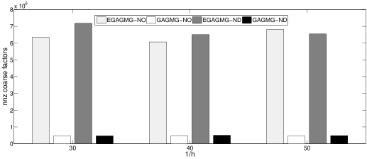
Figure 3: Comparison of no. of nonzeros for exact and inexact coarse grid solves for JUMP3D

Here again, the velocity field $\mathbf{a}$ is kept zero. We consider a $n\times n\times n$ uniform grid. The jump in the diagonal entries of the coefficient matrix is shown in Figure (3).

DCC1, 2D case: Same as DC1, 2D case above, except that the velocity is non-zero and it is given as $a(x)=(1000,1000)$.

DCC2, 3D case: Same as DC1, 3D case above, except that the velocity $a(x)=(1000,1000,1000)$.

Florida matrix market collection: The list of Florida matrix matrices are shown in Table (3). As we observe, all the problems are symmetric positive definite steaming from wide range of applications. For more on the properties of these matries, the reader is referred to [9].

Table 3: Forida matrix market matrices. Here SPD stands for symmetric positive definite.

Matrices	Kind	SPD	size	non-zeros
gyro_m	Model reduction problem	Yes	17361	340K
bodyy4	Structural problem	Yes	17546	121K
nd6k	2D/3D problem	Yes	18000	6.8M
bodyy5	Structural problem	Yes	18589	128K
wathen100	Random 2D/3D problem	Yes	30401	471K
wathen120	Random 2D/3D problem	Yes	36441	565K
torsion1	Duplicate optimization problem	Yes	40000	197K
obstclae	Optimization problem	Yes	40000	197K
jnlbrng1	Optimization problem	Yes	40000	199K
minsurfo	Optimization problem	Yes	40806	203K
gridgena	Optimization problem	Yes	48962	512K
crankseg_1	Structural problem	Yes	52804	10M
qa8fk	Acoustic problem	Yes	66127	1M
cfd1	Computational fluid dynamics	Yes	70656	1.8M
finan512	Economic problem	Yes	74752	596K
shallow_water1	Computational fluid dynamics	Yes	81920	327K
2cubes_sphere	Electromagnetic problem	Yes	101492	1.6M
Thermal_TC	Thermal problem	Yes	102158	711K
Thermal_TK	Thermal problem	Yes	102158	711K
G2_circuit	circuit simulation	Yes	150102	726K
bcsstk18	structural problem	Yes	11948	149K
cbuckle	structural problem	Yes	13681	676K
Pres_Poisson	Computational fluid dynamics	Yes	14822	715K

3.2 Comments on numerical results

Two version of GMG are shown, namely, GMG-NO which stands for GMG where smoother has natural ordering, and GMG-ND stands for GMG with smoother having nested dissection ordering. In particular, for GMG-ND, we first apply the nested dissection reordering and then the smoother is defined. We observe that after applying nested dissection reordering, the smoother which is ILU(0) in our case can be computed and applied in parallel. Since, in ILU(0), no pivoting is done, parallelizing ILU(0) after ND ordering leads to a parallel smoother. Certainly, not much parallelism is expected when the smoother is applied with natural ordering of unknowns. As mentioned before, for the coarse grid solve, we use ILU($10^{-4}$) to solve it inexactly. We do this inexact solve to see the effect of inexact solve in the iteration count and time. For AGMG, Gauss-Seidel smoothing is used, and the choice of the coarse grid is based on the strength of connection between nodes. Moreover, in AGMG, usual multilevel recursive approach is followed, i.e., going down the grid heirarchy untill the coarse grid is small enough (or it stops when it does not satisfy certain criteria) to be solved exactly.

We recall here that our aim is to compare the classical multi-grid approach implemented in AGMG with the two grid approach of GMG with the following ingredients

• Coarse grid based on graph matching (call to METIS)

• ILU(0) is the smoother (built in MATLAB)

• Coarse grid equation is solved inexactly (using built in ILU($t$) routine in MATLAB)

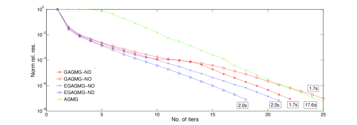
Figure 1: Convergence curve for Pres_Poisson for exact and inexact coarse grid solves. CPU time indicated inside small box.

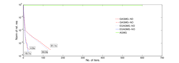
Figure 2: Convergence curve for DC3D $50\times 50\times 50$ for exact and inexact coarse grid solves. CPU time indicated inside small box.

In Tables (4), (5), (6), (7), (8), (9), (10), (11), (12), and (13), we have shown the iteration count and the total CPU time: setup time plus solve time, for values of $cf$ ranging from 3 to 8. For the values of $cf$ lying between 3 and 8, we can locate the value of $cf$ for which the CPU time is observed to be lowest, to do so, we had to vary $cf$ so that we do not miss a value of $cf$ for which the CPU time could be lowest. For 2D problems, we find that the AGMG method is several times faster than the GMG based methods. However, for 3D problems, the AGMG method does not converge at all. In contrast, GMG methods converges and shows mesh independent convergence rates for all values of $cf$. Considering 2D case first: the least CPU time for GMG-NO method is observed for $cf=3$. For GMG-ND method, the least CPU time is observed for $cf=2.5$ except for 2D $1200\times 1200$ problem for which the least CPU time occurs for $cf=3$. On the other hand, for EGMG-NO method, the least CPU time was observed when we had $cf=4$ for $800\times 800$ and $1200\times 1200$ problem, and the least CPU time for $1200\times 1200$ problem was obtained when $cf$ was equal to 6. For a smaller size 3D problem of $70\times 70\times 70$, the iteration count rather increases rapidly with the increasing value of $cf$. For smaller problems, it seems that a finer coarse grid is necessary. The reason for high iteration count may be due to the fact that for a given partial differential equation, the coefficient matrix becomes smoother as the resolution of the mesh is increased. In Figures 1 and 2, we find that the convergence curve for the respective exact and inexact methods are very similar, this also suggests a similar spectrum and probably a similar condition number. To find how close the approximated coarse matrix is to the exact coarse operator, in Table 24, we compare the relative error $\|LU-\tilde{L}\tilde{U}\|/\|LU\|$ for both natural and ND ordering. We find that the relative error is quite small, this is the reason why the direct and indirect versions converges in similar number of iterations. But since the inexact methods are relatively fast to build and apply, we save significant number of CPU time and storage requirement, see Figure (3) where an inexact solve needs about 10 times less storage compared to the exact solver.

In Tables (14), (15), (16), (17), (18), (19), (20), (21), and (22), we have similar plots for the test case DCC1. For this problem, we find that the AGMG method converges much faster compared to the GMG methods for both 2D and 3D problems, exception being the $120\times 120\times 120$ problem where the method fails to converge. However, we remind ourselves that GMG methods are implemented in Matlab, and thus they are expected to be faster when they are implemented in lower level languages such as Fortran or C. Thus, our prediction is that even for these problems where GMG shows larger CPU time, an implementation in Fortran may have the convergence time comparable with that of AGMG. Notably, for this test case, the iteration count decreases even more rapidly (compared to test case DC1) with the increase in the size of the problem.

The rule of thumb in the choice of coarse grid size is to increase the $cf$ value proportionally with the increasing size of the problem. For a smaller size problem with discontinous coefficients such as DC1 and DCC1, it is good to keep the $cf$ value small. The choice of drop tolerance in ILUT to be $10^{-6}$ worked well in practice and we did not encounter any breakdown. However, in case when the jumps are large, the fault tolerant mechanism such as the one discussed in the analysis section can be used.

Finally, in Table (25), we show some experiments with the Florida matrix market problems. We fixed the coarse grid size to be 4096. In general, for most of the problems, we find that the two-grid method is faster compared to AGMG, exception being, torsion1, obstclae, jnlbrng1, minsurfo, qa8fk, and shallow_water, where AGMG is about five times faster. For rest of the problems, GMG methods shows more robustness compared to AGMG. Comparing GMG-NO to GMG-ND, we find that GMG-NO converges faster with few exceptions. In Table (26), we present the numerical results with $cf=2.5$. A detailed investigation of the best coarse grid size for these problems deserves more effort and detailed study.

Table 4: Numerical results for DC1 problem with $cf=2.5$ using GMRES(30).

matrix	$h$	GMG-ND		GMG-NO		EGMG-NO		AGMG
		its	time	its	time	its	time	its	time
	1/800	23	25.5	17	17.4	16	38.7	27	6.3
2D	1/1000	23	45.5	18	30.3	18	82.0	37	14.1
	1/1200	24	70.8	20	48.2	18	159.5	37	18.2
	1/70	145	65.8	21	21.0	14	163.0	NC	NA
3D	1/100	191	306.5	26	141.0	ME	NA	NC	NA
	1/120	147	598.0	45	379.2	ME	NA	NC	NA

Table 5: Numerical results for DC1 problem with $cf=3$ using GMRES(30).

matrix	$h$	GMG-ND		GMG-NO		EGMG-NO		AGMG
		its	time	its	time	its	time	its	time
	1/800	28	24.7	20	16.8	19	22.8	27	6.3
2D	1/1000	29	50.4	19	25.6	19	25.5	37	14.1
	1/1200	26	65.8	19	37.6	20	70.8	37	18.2
	1/70	165	66.0	20	14.3	15	47.5	NC	NA
3D	1/100	191	314.1	25	94.2	16	839.2	NC	NA
	1/120	165	417.0	35	236.8	ME	ME	NC	NA

Table 6: Numerical results for DC1 problem with $cf=3.5$ using GMRES(30).

matrix	$h$	GMG-ND		GMG-NO		EGMG-NO		AGMG
		its	time	its	time	its	time	its	time
	1/800	33	30.6	28	22.7	22	19.9	27	6.3
2D	1/1000	36	50.9	23	28.6	22	33.8	37	14.1
	1/1200	34	72.7	23	42.2	22	54.8	37	18.2
	1/70	153	55.7	23	11.6	17	21.5	NC	NA
3D	1/100	200	221.8	32	58.6	23	254.8	NC	NA
	1/120	153	339.5	33	119.5	19	740.2	NC	NA

Table 7: Numerical results for DC1 problem with $cf=4$ using GMRES(30).

matrix	$h$	GMG-ND		GMG-NO		EGMG-NO		AGMG
		its	time	its	time	its	time	its	time
	1/800	44	34.8	26	20.6	24	19.7	27	6.3
2D	1/1000	37	49.8	25	30.1	25	33.2	37	14.1
	1/1200	37	72.3	28	51.1	27	53.8	37	18.2
	1/70	164	57.6	84	29.5	55	26.3	NC	NA
3D	1/100	212	235.8	27	44.5	19	116.3	NC	NA
	1/120	168	346.2	31	94.8	21	326.3	NC	NA

Table 8: Numerical results for DC1 problem with $cf=4.5$ using GMRES(30).

matrix	$h$	GMG-ND		GMG-NO		EGMG-NO		AGMG
		its	time	its	time	its	time	its	time
	1/800	43	32.7	27	20.5	27	21.1	27	6.3
2D	1/1000	44	53.9	28	33.9	27	33.4	37	14.1
	1/1200	41	74.0	27	47.5	29	55.6	37	18.2
	1/70	170	58.7	89	31.0	70	26.6	NC	NA
3D	1/100	205	215.4	28	40.9	22	63.3	NC	NA
	1/120	157	302.3	34	83.5	24	165.0	NC	NA

Table 9: Numerical results for DC1 problem with $cf=5$ using GMRES(30).

matrix	$h$	GMG-ND		GMG-NO		EGMG-NO		AGMG
		its	time	its	time	its	time	its	time
	1/800	46	34.4	32	24.4	30	24.2	27	6.3
2D	1/1000	47	56.8	32	37.9	34	39.2	37	14.1
	1/1200	51	86.8	30	53.8	29	53.6	37	18.2
	1/70	284	94.2	199	63.3	193	62.9	NC	NA
3D	1/100	206	280.9	30	55.2	23	60.5	NC	NA
	1/120	168	335.3	40	92.2	26	122.7	NC	NA

Table 10: Numerical results for DC1 problem with $cf=5.5$ using GMRES(30).

matrix	$h$	GMG-ND		GMG-NO		EGMG-NO		AGMG
		its	time	its	time	its	time	its	time
	1/800	51	37.0	33	23.5	33	23.9	27	6.3
2D	1/1000	52	61.3	34	37.6	33	37.8	37	14.1
	1/1200	50	84.2	33	54.3	32	55.3	37	18.2
	1/70	469	148.1	162	50.9	160	51.5	NC	NA
3D	1/100	219	222.9	148	146.2	109	117.0	NC	NA
	1/120	221	393.7	42	83.4	28	95.4	NC	NA

Table 11: Numerical results for DC1 problem with $cf=6$ using GMRES(30).

matrix	$h$	GMG-ND		GMG-NO		EGMG-NO		AGMG
		its	time	its	time	its	time	its	time
	1/800	55	41.4	36	25.2	36	25.2	27	6.3
2D	1/1000	56	65.8	36	40.0	36	40.0	37	14.1
	1/1200	55	92.9	36	56.1	36	56.8	37	18.2
	1/70	568	183.2	316	98.9	354	115.9	NC	NA
3D	1/100	208	213.5	103	100.4	94	101.1	NC	NA
	1/120	167	308.1	43	83.7	41	95.5	NC	NA

Table 12: Numerical results for DC1 for 2D and 3D problems with $cf=7$ using GMRES(30)

matrix	$h$	GMG-ND		GMG-NO		EGMG-NO		AGMG
		its	time	its	time	its	time	its	time
	1/800	68	41.9	51	25.8	41	27.2	27	6.3
2D	1/1000	68	73.5	41	36.9	41	40.9	37	14.1
	1/1200	73	112.0	41	59.4	41	60.0	37	18.2
	1/70	NC	NA	462	140.9	277	86.6	NC	NA
3D	1/100	566	542.2	266	249.9	255	239.0	NC	NA
	1/120	173	314.5	72	127.5	57	114.5	NC	NA

Table 13: Numerical results for DC1 for 2D and 3D problems with $cf=8$ using GMRES(30)

matrix	$h$	GMG-ND		GMG-NO		EGMG-NO		AGMG
		its	time	its	time	its	time	its	time
	1/800	77	48.3	48	30.9	48	30.9	27	6.3
2D	1/1000	76	74.6	46	46.8	46	47.2	37	14.1
	1/1200	77	108.6	46	67.0	45	65.9	37	18.2
	1/70	NC	NA	360	120.2	381	125.1	NC	NA
3D	1/100	NC	NA	454	441.4	440	426.5	NC	NA
	1/120	486	831.2	186	319.5	187	326.2	NC	NA

Table 14: Numerical results for DCC1 problem with $cf=2.5$ using GMRES(30).

matrix	$h$	GMG-ND		GMG-NO		EGMG-NO		AGMG
		its	time	its	time	its	time	its	time
	1/800	54	45.3	49	36.6	18	14.2	27	6.3
2D	1/1000	75	90.4	60	73.7	19	83.0	37	14.1
	1/1200	51	101.4	40	61.1	21	165.6	37	18.2
	1/70	100	50.3	14	17.4	14	161.6	16	3.4
3D	1/100	139	223.8	15	100.8	ME	NA	15	8.8
	1/120	123	471.3	15	264.2	ME	NA	NC	NA

Table 15: Numerical results for DCC1 problem with $cf=3$ using GMRES(30).

matrix	$h$	GMG-ND		GMG-NO		EGMG-NO		AGMG
		its	time	its	time	its	time	its	time
	1/800	28	24.7	20	16.8	19	22.8	27	6.3
2D	1/1000	29	50.4	19	25.6	19	25.5	37	14.1
	1/1200	26	65.8	19	37.6	20	70.8	37	18.2
	1/70	113	48.7	15	10.6	15	46.9	16	3.4
3D	1/100	153	207.3	17	53.2	17	681.8	15	8.8
	1/120	135	337.8	17	119.7	ME	ME	NC	NA

Table 16: Numerical results for DCC1 problem with $cf=3.5$ using GMRES(30).

matrix	$h$	GMG-ND		GMG-NO		EGMG-NO		AGMG
		its	time	its	time	its	time	its	time
	1/800	47	36.5	32	25.1	27	24.7	27	6.3
2D	1/1000	52	64.0	41	44.4	28	42.9	37	14.1
	1/1200	44	80.8	30	57.8	27	65.5	37	18.2
	1/70	129	48.6	16	8.7	16	21.0	16	3.4
3D	1/100	171	194.2	18	36.5	18	248.0	15	8.8
	1/120	150	325.0	18	78.3	18	744.7	NC	NA

Table 17: Numerical results for DCC1 for 2D and 3D problems with $cf=4$ using GMRES(30)

matrix	$h$	GMG-ND		GMG-NO		EGMG-NO		AGMG
		its	time	its	time	its	time	its	time
	1/800	57	43.8	32	24.8	31	26.2	27	6.3
J2D	1/1000	53	56.4	38	41.7	35	43.7	37	14.1
	1/1200	52	81.3	39	61.9	38	66.1	37	18.2
	1/70	138	52.0	26	12.4	26	15.8	16	3.4
3D	1/100	182	191.2	19	31.1	19	109.9	15	8.8
	1/120	170	308.8	20	61.2	19	312.9	NC	NA

Table 18: Numerical results for DCC1 for 2D and 3D problems with $cf=4.5$ using GMRES(30)

matrix	$h$	GMG-ND		GMG-NO		EGMG-NO		AGMG
		its	time	its	time	its	time	its	time
	1/800	76	53.9	39	27.6	37	27.5	27	6.3
J2D	1/1000	74	82.2	39	43.9	38	44.4	37	14.1
	1/1200	64	112.6	39	64.1	37	65.6	37	18.2
	1/70	151	53.5	38	16.1	38	18.1	16	3.4
3D	1/100	210	234.6	21	31.1	21	66.0	15	8.8
	1/120	180	363.6	22	61.5	22	169.2	NC	NA

Table 19: Numerical results for DCC1 for 2D and 3D problems with $cf=5$ using GMRES(30)

matrix	$h$	GMG-ND		GMG-NO		EGMG-NO		AGMG
		its	time	its	time	its	time	its	time
	1/800	88	60.95	45	29.0	43	28.1	27	6.1
2D	1/1000	80	77.2	48	48.6	49	50.8	37	13.2
	1/1200	81	114.0	43	64.4	42	64.7	37	18.3
	1/70	169	59.4	60	22.8	60	24.0	16	3.4
3D	1/100	224	219.8	22	29.7	22	45.3	15	8.8
	1/120	195	340.35	23	56.8	23	111.0	NC	NA

Table 20: Numerical results for DCC1 for 2D and 3D problems with $cf=5.5$ using GMRES(30)

matrix	$h$	GMG-ND		GMG-NO		EGMG-NO		AGMG
		its	time	its	time	its	time	its	time
	1/800	107	73.0	50	33.7	48	32.7	27	6.1
2D	1/1000	100	107.8	50	55.3	49	52.7	37	13.2
	1/1200	90	148.7	48	74.2	47	72.8	37	18.3
	1/70	282	100.6	65	24.5	70	26.7	16	3.4
3D	1/100	240	260.6	44	52.0	45	63.2	15	8.8
	1/120	223	405.1	24	56.9	24	84.5	NC	NA

Table 21: Numerical results for DCC1 for 2D and 3D problems with $cf=6$ using GMRES(30)

matrix	$h$	GMG-ND		GMG-NO		EGMG-NO		AGMG
		its	time	its	time	its	time	its	time
	1/800	132	79.7	56	36.7	56	37.0	27	6.3
2D	1/1000	117	112.4	55	56.1	54	55.2	37	14.1
	1/1200	111	152.5	55	80.9	53	77.9	37	18.2
	1/70	261	88.9	90	32.2	88	31.5	16	3.4
3D	1/100	256	250.4	41	47.1	41	51.3	15	8.8
	1/120	225	384.6	26	61.7	27	78.9	NC	NA

Table 22: Numerical results for DCC1 problem with $cf=7$ using GMRES(30).

matrix	$h$	GMG-ND		GMG-NO		EGMG-NO		AGMG
		its	time	its	time	its	time	its	time
	1/800	184	112.3	67	42.7	65	42.0	27	6.3
2D	1/1000	173	162.6	69	68.1	67	67.5	37	14.1
	1/1200	397	530.4	67	97.6	64	95.2	37	18.2
	1/70	351	117.5	109	32.6	109	36.3	16	3.4
3D	1/100	301	296.2	80	82.8	78	81.8	15	8.8
	1/120	257	440.0	29	69.7	29	74.5	NC	NA

Table 23: Numerical results for DCC1 problem with $cf=8$ using GMRES(30).

matrix	$h$	GMG-ND		GMG-NO		EGMG-NO		AGMG
		its	time	its	time	its	time	its	time
	1/800	266	171.3	82	51.5	83	54.2	27	6.3
2D	1/1000	229	225.6	84	81.0	83	79.8	37	14.1
	1/1200	218	297.7	81	112.4	78	107.8	37	18.2
	1/70	502	161.0	123	41.0	115	37.9	16	3.4
3D	1/100	449	445.9	105	102.4	104	101.8	15	8.8
	1/120	294	517.2	57	109.8	57	112.2	NC	NA

Table 24: Comparison of exact and inexact coarse operators. Here NO stands for natural ordering and ND stands for nested dissection ordering

Problem	1/$h$	$\frac{\|LU-\tilde{L}\tilde{U}\|}{\|LU\|}$ for NO	$\frac{\|LU-\tilde{L}\tilde{U}\|}{\|LU\|}$ for ND
	1/30	$7.5e^{-5}$	$7.8e^{-5}$
JUMP3D	1/40	$8.3e^{-5}$	$7.2e^{-5}$
	1/50	$7.0e^{-5}$	$1.1e^{-4}$

Table 25: Numerical results for Florida matrix market collection.

matrix	$N_{c}$	GMG-ND		GMG-NO		AGMG
		its	time	its	time	its	time
gyto_m	4096	111	5.2	137	7.0	$>600$	NA
bodyy4	4096	54	1.8	19	0.4	$>600$	NA
nd6k	4096	NC	NA	89	21.3	MEM	NA
bodyy5	4096	115	4.6	30	0.7	-	-
wathen100	4096	12	1.4	9	0.7	11	4.1
wathen120	4096	12	1.3	9	0.9	11	35.0
torsion1	4096	13	0.99	9	0.6	6	0.1
obstclae	4096	13	0.9	9	0.6	6	0.1
jnlbrng1	4096	22	1.5	11	0.7	11	0.1
minsurfo	4096	16	1.0	11	0.6	8	0.1
gridgena	4096	310	81.4	189	34.0	$>600$	NA
crankseg_1	4096	60	22.3	76	26.2	334	69.1
qa8fk	4096	11	4.9	12	3.6	15	1.3
cfd1	4096	145	45.1	127	32.0	MEM	NA
finan512	4096	7	1.8	7	1.2	4	106.0
shallow_water1	4096	6	1.3	6	0.8	4	0.1
2cubes_sphere	4096	6	3.9	6	2.5	7	8.6
Thermal_TC	4096	6	2.03	7	1.4	MEM	NA
Thermal_TK	4096	22	3.6	23	3.5	80	5.0
G2_circuit	4096	32	7.7	24	4.2	91	5.9
bcsstk18	4096	232	11.6	111	3.7	$>600$	NA
cbuckle	4096	41	2.3	62	3.0	493	18.7
Pres_Poisson	4096	21	1.7	24	1.7	24	16.8

Table 26: Numerical results for Florida matrix market collection with $cf=2.5$

matrix	GMG-ND		EGMG-ND		GMG-NO		EGMG-NO		AGMG
	its	time	its	time	its	time	its	time	its	time
gyto_m	271	4.1	319	4.6	465	6.9	562	7.3	NC	NA
bodyy4	56	0.9	56	0.9	19	0.3	19	0.4	NC	NA
nd6k	NC	NA	NC	NA	NC	NA	NC	NA	ME	NA
bodyy5	135	1.8	137	1.8	31	0.6	31	0.6	1	245.4
wathen100	12	1.0	12	1.1	9	0.6	9	0.7	11	4.3
wathen120	12	1.2	12	1.3	9	0.8	9	0.8	11	7.0
torsion1	14	0.9	14	1.0	10	0.5	10	0.6	6	0.1
obstclae	14	0.9	14	1.0	10	0.5	10	0.6	6	0.1
jnlbrng1	25	1.3	24	1.3	12	0.6	12	0.6	11	0.2
minsurfo	18	1.0	18	1.2	11	0.5	12	0.6	7	0.2
gridgena	NC	NA	NC	NA	307	10.3	308	9.2	NC	NA
crankseg_1	74	21.4	109	31.6	99	25.5	87	29.0	468	96.0
qa8fk	12	4.9	11	5.8	11	3.6	10	4.4	15	1.3
cfd1	439	37.0	442	38.3	259	23.0	255	30.5	ME	NA
finan512	6	1.8	6	1.9	7	1.2	7	1.3	4	106.0
shallow_water1	6	1.4	6	2.3	6	0.9	6	1.7	4	0.1
2cubes_sphere	6	4.4	7	8.6	5	3.0	5	15.2	7	8.6
Thermal_TC	6	2.2	6	2.5	6	1.5	6	1.9	ME	NA
Thermal_TK	NC	NA	NC	NA	NC	NA	NC	NA	NC	NA
G2_circuit	28	7.3	21	7.7	21	4.7	15	5.0	74	4.8
bcsstk18	NC	NA	NC	NA	166	1.9	169	2.0	F1	NA
cbuckle	54	1.5	54	1.5	247	4.0	198	3.7	F1	NA
Pres_Poisson	24	1.0	22	1.0	26	1.0	26	1.0	24	21.2

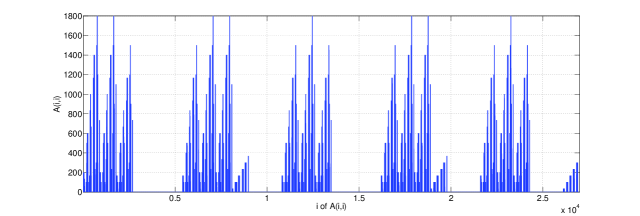
Figure 4: Jump in the diagonal entries of DC3D $30\times 30\times 30$ matrix when $\kappa(x)$ values are kept as $10^{3}$

4 Conclusion

We have proposed a two grid approach GAGMG with following ingredients

• Coarse grid based on graph matching

• ILU(0) is the smoother with natural or nested dissection reordering

• Coarse grid equation is solved inexactly

We compared out approach with the classical AGMG scheme. On comparison, we found that the new strategy seems to be robust with a very modest coarse grid size which is further solved cheaply by performing an inexact solve. One of the aim of this work was to provide a practical, easy to implement, yet robust two-grid methods.

We have tried only the sequential version of our method, in future, we would like to implement the method in parallel with a parallel inexact solve strategy.

5 Acknowledgement

Many thanks to Université libre de Bruxelles for an ideal environment and the fond de la reserche scientifique (FNRS) Ref: 2011/V 6/5/004-IB/CS-15 that made this work possible.

References

- [1] Y. Achdou and F. Nataf, Low frequency tangential filtering decomposition, Numer. Linear Algebra Appl. 14 (2006), pp 129-147.
- [2] J.I. Aliaga, M. Bollhofer, A. Martin, and E. Quintana-Orti, ILUPACK, Invited book chapter in Springer Encyclopedia of parallel computing, David Padua (ed.), Springer, to appear, ISBN: 978-0-387-09765-7.
- [3] S. F. Ashby, M. J. Holst, T. A. Manteuffel, and P. E. Saylor, The role of inner product in stopping criteria for conjugate gradient iterations, BIT, 41 (2001), pp 26-52.
- [4] R. Barret, M. Berry, T. F. Chan, J. Demmel, J. Donato, J. Dongarra, V. Eijkhout, R. Pozo, C. Romine, and H. Van der Vorst, Templates for the solution of linear systems: Building blocks for iterative methods, 2nd Edition, SIAM, 1994, Philadelphia, PA.
- [5] M. Benzi and A. M. Tuma, A comparative study of sparse approximate inverse preconditioners, Applied Numerical Mathematics 30 (1999) 305-340.
- [6] D. Braess, Towards algebraic multigrid for elliptic problems of second order, Computing 55(4) (1995) 379-393.
- [7] J. H. Bramble, J. E. Pasciak, and A. T. Vassilev, Analysis of non-overlapping domain decomposition algorithms with inexact solves, Math. Comp. 67 (1998), pp 1-19.
- [8] T. Davis, Direct methods for sparse linear systems, SIAM, Philadelphia, 2006.
- [9] T.A. Davis, Y. Hu, The university of Florida sparse matrix collection, ACM Transactions on Mathematical Software, (to appear).
- [10] N. J. Higham, Accuracy and stability of numerical algorithms, second edition, SIAM 2002, ISBN 0-89871-521-0.
- [11] H. Kim, J. Xu, and L. Zikatanov, A multigrid method based on graph matching for convection-diffusion equations, Numer. Linear Algebra Appl., 10(2003), pp. 181-195.
- [12] G. Karypis, V. Kumar, A fast and high quality multilevel scheme for partitioning irregular graphs, SIAM J. Sci. Comp., (1999), 359-392.
- [13] P. Kumar, L. Grigori, F. Nataf, Q. Niu, Combinative preconditioning based on relaxed nested factorization and tangential filtering preconditioner, INRIA Tech. report RR-6955.
- [14] Z. Li, Y. Saad, and M. Sosonkina, pARMS: a parallel version of the algebraic recursive multilevel solver, Num. Lin. Alg. Appl., 10, (2003), 485-509.
- [15] J.A. Meijerink and H. A. van der Vorst, An iterative solution method for linear system of which the coefficient matrix is a symmetric M-matrix, Math. Comp. 31 (1977), pp 148-162.
- [16] Y. Notay, An aggregation based algebraic multigrid method, Electronic transaction on Numerical analysis, 37 (2010), pp 123-146.
- [17] R. Nabben and C. Vuik, A comparison of deflation and coarse grid correction applied to porous media flow, SIAM J. NUMER. ANAL. 42(4) (2004), pp. 1631-1647.
- [18] Y. Notay, Convergence analysis of perturbed two-grid and multigrid methods, SIAM J. Matrix Anal. Appl., 45, (2007), pp 1035-1044.
- [19] Y. Notay, AGMG: Agregation based AMG, availalable at: http://homepages.ulb.ac.be/~ynotay
- [20] M. Rasquin, H. Deconinck, and G. Degrez, FLEXMG: A new library of multigrid preconditioners for a spectral/finite element incompressible flow solver, Int. J. Numer. Meth. Engng, 82 (2010), pp 1510-1536.
- [21] J. W. Ruge and K. Stüben, Algebraic multigrid, Multigrid Methods, Frontiers of Applied Mathematics, vol. 3. SIAM Philadelphia, PA (1987) 73-130.
- [22] Y. Saad, Iterative Methods for Sparse Linear Systems, PWS publishing company, Boston, MA, 1996.
- [23] Y. Saad and B. Suchomel, ARMS : An algebraic recursive multilevel solver for general sparse linear systems, NLAA, 9, (2002), pp.359-378.
- [24] Y. Saad, Matlab suite, Available online at: http://www-users.cs.umn.edu/~saad/software/.
- [25] K. Stüben, A review of algebraic multigrid, J. Comput. Appl. Math. and applied mathematics, 128(1-2) (2001) 281-309, Numerical analysis 2000, vol. VII, Partial differential equations.
- [26] U. Trottenberg, C. W. Oosterlee, and A. Schüller, Multigrid, Academic Press Inc. San Diego, CA, 2001, with contributions by Brandt A, Oswald P, and Stüben K.
- [27] C. Wagner and G. Wattum, Adaptive filtering Numer. Math., 78, 1997 pp.305-382.
- [28] C. Wagner, Tangential frequency filtering decompositions for unsymmetric matrices Numer. Math., 78, 1997 pp.143-163.
- [29] C. Wagner, Tangential frequency filtering decompositions for symmetric matrices Numer. Math., 78, 1997 pp.119-142.
- [30] R. Wienands, W. Joppich, Practical Fourier analysis for multigrid methods, Taylor and Francis Inc., 2004